NT receptor (Pi) mRNA was observed in more than 25% of the ... neurons in the dorsal horn, and (3) NT-IR cell bodies and fibers in lam- inae I-II. .... gland Nuclear), and DTT was added to a final concentration of 10 mM. The specific activities .....
Oct 4, 2016 - [20] G. Simonyi, âPerfect graphs and graph entropy. An updated survey,â J. Ramirez-Alfonsin, B. Reed (Eds.), Perfect Graphs, pp. 293-328. John.
networks. Franco Blanchini1, Daniele Casagrande2, Giulia Giordano3, and Umberto Viaro2 ... 1 Dipartimento di Scienze Matematiche, Informatiche e Fisiche,. Universit`a ...... [26] W. Ren, R. W. Beard, and E. Atkins, âInformation consensus.
Jul 25, 2014 - with or without 10 µM dicoumarol present in the as- say system. The dicoumarol-sensitive part of the ac- tivity was calculated as the slope of the ...
generalized r, q distribution function. Such case is of interest when the solar wind is streaming through the cometary plasma in the presence of interstellar dust ...
Jun 4, 2008 - Melnitchouk, Donna Naples, Mary Hall Reno, Voica A. Radescu, and Martin Tzanov for valuable discussions, and BNL, CERN, and Fermilab ...
Jul 6, 2011 - (9) and (10). Thus, we can express the PDF for the MRW model as. PMRW (β,N; Z) â¡ Ïβ(z),. (11) z = Z. Ze . We see that Ze defines the scale for ...
Sep 21, 2011 - were recorded with an acquisition rate of 4 Hz. Metafluor software ... plug-in; www.macbiophotonics.ca) and custom-written programs in.
Aug 7, 2012 - Journal of Statistical Software. 3 to the best of our knowledge, only two methods have been investigated in the distribution estimation context: ...
stars in Ï Centauri from a catalogue of Washington M, T2 and DDO51 photometry covering over .... Discussion: What is Omega Centauri? It is well known that Ï ...
that enables sampling from different parts of the liver for func- .... MR injector System; Medrad, Pittsburgh, PA, USA), at an infusion rate of 2 ml/s, followed ...
Dec 15, 1981 - A method of interpreting radial distribution functions (RDF) of amorphous metals is proposed in which the role of the local atomic structure is ...
Radial Distribution Function for Hard-Sphere Fermions at Zero and Finite Temperatures. J unzo CHIHARA. Japan Atomic Energy Research Institute. Tokai-mura ...
Abstractâ In this work, a new iris recognition algorithm based on tonal distribution of iris images is introduced. During the process of identification probability ...
function f(r,k,t), obtained by solving the Boltzmann transport equation (BTE) ..... 2 P.J. Price, âMonte Carlo calculation of electron transport in solids,â Semiconductors and ... 3 C. Jacoboni and P. Lugli, The Monte Carlo Method for Semiconduct
Frommhold [8] (drift velocity); Raja Rao and Govinda Raju [9] (α/N and DT/μ) and Moruzzi [10]. (α/N); Rees and Jory [11] and Lakshminarasimha and Lucas [12] ...
Ramu Yerukala and Naveen Kumar Boiroju. Abstract: This paper presents three new approximations to the cumulative distribution function of standard normal ...
Aug 18, 2015 - The active layer of organic solar cells is based on the concept of ... of free charge carriers at the metal/organic (M/O) interfaces from ... continuity equation has been solved using Laplace transform and the ... Ytterbium (20 nm) lay
F. Gerbier,â J. H. Thywissen,â S. Richard, M. Hugbart, P. Bouyer, and A. Aspect. Laboratoire ..... [13] I. Bloch, T. W. Hänsch, and T. Esslinger, Nature 403,.
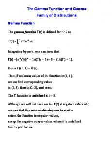
The Gamma Function and Gamma. Family of Distributions. Gamma Function. The
gamma function Γ(t) is defined for t > 0 as. ∫. ∞. −. −. =Γ. 0. 1 . )( dx ex.
A Statistical Distribution Function of. Wide Applicability. BY WALODDI WEIBULL,
1 STOCKHOLM, SWEDEN. This paper discusses the applicability of statistics to ...
Journal of Applied Crystallography covers a wide range of crystallographic topics from the viewpoints of both techniques and theory. The journal presents ...
Dec 12, 2002 - good traffic connections with the hinterland, and. - good maritime connections. The entire potential of a seaport and its optimal performing of the ...
DISTRIBUTION SEMIGROUPS ON FUNCTION. SPACES WITH SINGULARITIES AT ZERO. Stevan Pilipovic1, Fikret Vajzovic2, Mirjana Vukovic3. Abstract.
Figure 1- approximation of sin distribution (red) vs original (blue). Page 4. Figure 2 â Normal bell curve (green) vs various approximations.
The scope is to evaluate the CDF (complementary distribution function) of a sum of two signals (one Gaussian, one CW). 𝑐𝑑𝑓𝑖 stands for cdf of interferer and should be a function with 𝜎 and 𝑎 parameters. Beyond are the considerations leading to the need of cdf evaluation. There are two signals adding in the propagation channel. First one is AWGN, having its pdf: 𝑝𝑛 (𝑥) =
1 √2𝜋𝜎
𝑒
−
𝑥2 2𝜎 2
Second is a CW (sinus) interferer, having some arcsin pdf:
1
𝑝𝑠 (𝑥) = 𝜋 ∙
1 √𝑎 2 −𝑥 2
, with 𝑥 2 < 𝑎2
This is not standard arcsin pdf (which can be seen in the link below), but a similar one http://www.math.uah.edu/stat/special/Arcsine.html . Arcsiuns distribution is a particular case of beta distribution. Both signal are zero average, so there are only two parameters: σ for normal distribution and a for arcsinus – which is in fact the amplitude of the CW interferer. Also, one can observe that 𝑝𝑠 (𝑥) has an elementary primitive, namely
1 𝑥 𝑎𝑟𝑐𝑠𝑖𝑛 . 𝜋 𝑎
Pdf of the interferer can be obtained from the convolution of the two distributions: 𝑝𝑖 = 𝑝𝑛 ∗ 𝑝𝑠 So interferer pdf is then: 𝑝𝑖 (𝑥) =
1 √2𝜋 3 𝜎
𝑎
∫
(𝑥−𝑡)2 − 𝑒 2𝜎2
−𝑎 √𝑡
2
− 𝑎2
𝑑𝑡
probably transcendental. Integration limits are finite since out of −𝑎. . . +𝑎 sinus distribution is zero (the pdf is bounded). Maybe it will be possible to use some of convolution properties in relation with an integral transform (the transform of convolution is the product of convolution terms transform). For determining influence of interferer over BER there is necessary to calculate either tail function, either cdf: 𝑥
𝑐𝑑𝑓𝑖 (𝑥) = ∫ 𝑝𝑖 (𝑡)𝑑𝑡 −∞
There is not mandatory an exact calculation, a decent approximation should be OK. Here comes a suggestion of approximation of the convolution product (not necessarily the best one ):
1) Normal distribution 2
Instead of 𝑝𝑛 (𝑥) =
𝑥 1 − 2 2𝜎 𝑒 √2𝜋𝜎
we can use approximation 𝑎𝑛 (𝑥) =
1 1 2 4 √2𝜋𝜎 1+( 𝑥 ) +1( 𝑥 ) √2𝜎
4 √2𝜎
2) Sinus pdf 1
Instead of 𝑝𝑠 (𝑥) = 𝜋 ∙
1 √𝑎 2 −𝑥 2
we can use approximation 𝑎𝑠 (𝑥) =
1 𝑎 ∙ 𝜋 𝑎 2 −𝑥 2
3) Now convolution integral is 4) 𝑝𝑑𝑓(𝑥) = 𝑎𝑛 (𝑥) ∗ 𝑎𝑠 (𝑥) ≅
We used first function as sliding part, since second function is bounded to (−𝑎, 𝑎). If this is not solvable, further simplification can be done: 1. Quit the 4th grade term 2. Adjust the 4th grade term in order to lead denominator to a perfect square 5) CDF, our final result: 𝑥
𝑐𝑑𝑓(𝑥) = ∫ 𝑝𝑑𝑓(𝑡)𝑑𝑡 −∞
Attached pictures are graphs of approximate functions vs original functions, in order to create a view of approximation functions.
Figure 1- approximation of sin distribution (red) vs original (blue)
Figure 2 – Normal bell curve (green) vs various approximations