Oct 4, 2016 - [20] G. Simonyi, âPerfect graphs and graph entropy. An updated survey,â J. Ramirez-Alfonsin, B. Reed (Eds.), Perfect Graphs, pp. 293-328. John.
Broadcast Function Computation with Complementary Side Information Jithin Ravi and Bikash Kumar Dey
arXiv:1610.00867v1 [cs.IT] 4 Oct 2016
Department of Electrical Engineering Indian Institute of Technology Bombay {rjithin,bikash}@ee.iitb.ac.in
Abstract—We consider the function computation problem in a three node network with one encoder and two decoders. The encoder has access to two correlated sources X and Y . The encoder encodes X n and Y n into a message which is given to two decoders. Decoder 1 and decoder 2 have access to X and Y respectively, and they want to compute two functions f (X, Y ) and g(X, Y ) respectively using the encoded message and their respective side information. We want to find the optimum (minimum) encoding rate under the zero error and �-error (i.e. vanishing error) criteria. For the special case of this problem with f (X, Y ) = Y and g(X, Y ) = X, we show that the �error optimum rate is also achievable with zero error. This result extends to a more general ‘complementary delivery index coding’ problem with arbitrary number of messages and decoders. For other functions, we show that the cut-set bound is achievable under �-error if X and Y are binary, or if the functions are from a special class of ‘compatible’ functions which includes the case f = g.
I. I NTRODUCTION We consider the broadcast function network with complementary side information as shown in Fig. 1. Here, (Xi , Yi ) is an i.i.d. discrete random process with an underlying probability mass function pXY (x, y). An encoder encodes X n and Y n into a message, which is given to two decoders. Decoder 1 and decoder 2 have side information X and Y respectively, and want to compute Z1 = f (X, Y ) and Z2 = g(X, Y ) respectively. We study this problem under �-error and zero error criteria. We are interested in finding the optimum broadcast rate in both cases. Xn Decoder 1 X n, Y n
Zˆ1n
Encoder Decoder 2
Zˆ2n
Yn
Fig. 1: Function computation in broadcast function network with complementary side information. Here Z1 = f (X, Y ), Z2 = g(X, Y ). We first consider a special case of the problem with Z1 = Y and Z2 = X, known as the complementary delivery problem. This special case is an instance of index coding problem
with two messages. This problem has been addressed under noisy broadcast channel in [1]–[3] for �-error recovery of the messages. In contrast to their model of independent messages, we consider correlated messages over a noiseless broadcast channel. Lossy version of this problem was studied in [4], [5]. For the lossless case, the optimal �-error rate can be shown to be max{H(Y |X), H(X|Y )} using the Slepian-Wolf result. We show that this rate is also achievable with zero error. We then extend this to n random variables which can also be considered as a special case of the index coding problem. Here, the server has messages X1 , . . . , XK and there are m receivers. Each receiver has a subset of {X1 , . . . , XK } as side information, and all the receivers want to recover all the random variables that it does not have access to. We call this setup as complementary delivery index coding problem. Cutset bound in this case can be shown to be achievable for �-error using the Slepian-Wolf result. We show that this rate is also achievable with zero error. Next we address the function computation problem shown in Fig. 1, where each decoder wants to recover a function of the messages. For �-error criteria, we give a single letter characterization of the optimal broadcast rate when either (i) Z1 = Z2 , (ii) X, Y are binary random variables, or (iii) Z1 , Z2 belong to a special class of ‘compatible’ functions (defined in Section II). For zero error criteria with variable length coding, we give single letter upper and lower bounds for the optimal broadcast rate. In contrast to correlated messages in our model, most work on index coding consider independent messages. On the other hand, in index coding problems in general, each receiver wants to recover an arbitrary subset of the messages. The goal is to minimize the broadcast rate of the message sent by the server (see [6]- [10] and references therein). For correlated sources, index coding problem has been studied for �-error where the receivers demand their messages to be decoded with �-error (see for example [11]). They gave an inner bound, and showed that it is tight for three receivers. To the best of our knowledge, index coding problem has not been considered for correlated sources with zero error. When the sources are independent and uniformly distributed, it was shown that the optimal rate for zero error and �-error are the same [12]. Our result extends this to correlated sources with arbitrary distribution in the specific case of complementary delivery. The technique followed in [12] does not directly extend to correlated sources.
The paper is organized as follows. In Section II, we present our problem formulation and some definitions. We provide the main results of the paper in Section III. Proof of the results are presented in Section IV. II. P ROBLEM FORMULATION AND DEFINITIONS A. Problem formulation: function computation There are one encoder and two decoders for the function computation problem shown in Fig 1. A (2nR , n) code for variable length coding consists of one encoder φ :X n × Y n −→ {0, 1}∗ and two decoders ψ1 :φ(X n × Y n ) × X n −→ Z n1 , n
n
n
ψ2 :φ(X × Y ) × Y −→
Z n2 .
(1) (2)
Here {0, 1}∗ denotes the set of all finite length binary sequences and we assume that the encoding is prefix free. Let us define Zˆ1n = ψ1 (φ(X n , Y n ), X n ) and Zˆ2n = ψ2 (φ(X n , Y n ), Y n ). The probability of error for a n length code is defined as Pe(n) , P r{(Zˆ1n , Zˆ2n ) 6= (Z1n , Z2n )}
(3)
The rate of the code is defined as 1 X P r(xn , y n ) | φ(xn , y n ) |, R = n n n (x ,y )
where | φ(xn , y n ) | denotes the length of the encoded sequence φ(xn , y n ). A rate R is said to be achievable with zero error if there is a zero-error code of some length n with (n) rate R and Pe = 0. Let R0n denote the optimal zero error rate for n length code. Then the optimal zero error rate R0∗ is defined as R0∗ = lim R0n . n→∞
A fixed length (2nR , n) code consists of one encoder map n
n
φ :X × Y −→ {1, 2, . . . , 2
nR
}
and the two decoder maps as defined in (1), (2). A rate R is said to be achievable with �-error if there exists (n) a sequence of (2nR , n) codes for which Pe → 0 as n → ∞. The optimal broadcast rate in this case is the infimum of the set of all achievable rates and it is denoted by R�∗ . B. Problem formulation: Index coding Let H(i) denote the indices of the messages that receiver i has and let XH(i) denote their corresponding values. Let us denote the complement of the set H(i) by H c (i). The set of messages that receiver i has, is denoted by XH(i) . The set of messages receiver i wants is XW (i) . For the complementary delivery index coding problem, W (i) = H c (i). The encoder, decoders, probability of error, achievable rate, etc. are defined similarly as before.
C. Graph theoretic definitions Let G be a graph with vertex set V (G) and edge set E(G). A set I ⊆ V (G) is called an independent set if no two vertices in I are adjacent in G. Let Γ(G) denote the set of all independent sets of G. A clique of a graph G is a complete subgraph of G. A clique of the largest size is called a maximum clique. The number of vertices in a maximum clique is called clique number of G and is denoted by ω(G). The chromatic number of G, denoted by χ(G), is the minimum number of colors required to color the graph G. A graph G is said to be perfect if for any vertex induced subgraph G0 of G, ω(G0 ) = χ(G0 ). Note that the vertex disjoint union of perfect graphs is also perfect. The n-fold OR product of G, denoted by G∨n , is defined by V (G∨n ) = (V (G))n and E(G∨n ) = {(v n , v 0n ) : (vi , vi0 ) ∈ E(G) for some i}. The n-fold AND product of G, denoted by G∧n , is defined by V (G∧n ) = (V (G))n and E(G∧n ) = {(v n , v 0n ) : either vi = vi0 or (vi , vi0 ) ∈ E(G) for all i}. For a graph G and a random variable X taking values in V (G), (G, X) represents a probabilistic graph. Chromatic entropy [17] of (G, X) is defined as Hχ (G, X) = min{H(c(X)) : c is a coloring of G}. Let W be distributed over the power set 2X . The graph entropy of the probabilistic graph (G, X) is defined as HG (X) =
min
X∈W ∈Γ(G)
I(W ; X),
(4)
where Γ(G) is the set of all independent sets of G. Here the minimum is taken over all conditional distributions pW |X which are non-zero only for X ∈ W . The following result was shown in [17]. lim
n→∞
1 Hχ (G∨n , X n ) = HG (X). n
(5)
The complementary graph entropy of (G, X) is defined as ¯ G (X) = lim lim sup 1 log2 {χ(G∧n (TPn ,� ))}, H X �→0 n→∞ n where TPnX ,� denotes the �-typical set of length n under the distribution PX . It was shown in [18] that 1 ¯ G (X). Hχ (G∧n , X n ) = H n→∞ n lim
(6)
To address the function computation problem, we define some suitable graphs. Let SX n Y n denote the support set of (X n , Y n ). A rook’s graph defined over X × Y has its vertex set X × Y and edge set {((x, y), (x0 , y 0 )) : x = x0 or y = y 0 , but (x, y) 6= (x0 , y 0 )}. For functions Z1 = f (X, Y ), Z2 = g(X, Y ) defined over X × Y, we now define a graph called Z1 Z2 -modified rook’s graph which is similar to the f -modified rook’s graph defined in [14]. 1 Z2 Definition 1 Z1 Z2 -modified rook’s graph GZ is a subXY graph of the rook’s graph on X × Y, which has its vertex
Xn
set SXY , and two vertices (x1 , y1 ) and (x2 , y2 ) are adjacent if and only if
Decoder 1 X n, Y n
1) x1 = x2 and f (x1 , y1 ) 6= f (x2 , y2 ),
Encoder
or 2) y1 = y2 and g(x1 , y1 ) 6= g(x2 , y2 ).
Decoder 2
Example 1 Let us consider a doubly symmetric binary source (DSBS(p)) (X, Y ) where pX,Y (0, 0) = pX,Y (1, 1) = (1−p)/2 and pX,Y (0, 1) = pX,Y (1, 0) = p/2, and functions Z1 , Z2 given by Z1 = X · Y � Y Z2 = X
(7) if Y = 0 if Y = 1,
(8)
Z1 Z2 -modified rook’s graph of these functions is shown in Fig. 2a. 1 Z2 Next we extend the definition of GZ to n instances: XY
Z1 Z2 Definition 2 GXY (n) has its vertex set SX n Y n , and two n n vertices (x , y ) and (x0n , y 0n ) are adjacent if and only if
1) xn = x0n and f (xi , yi ) 6= f (x0i , yi0 ) for some i, or 2) y n = y 0n and g(xi , yi ) 6= g(x0i , yi0 ) for some i. n n 1 Z2 Clearly, GZ XY (n) is the Z1 Z2 -modified rook’s graph on the vertex set SX n Y n . We note here from the definitions that Z1 Z2 ∨n 1 Z2 GZ . XY (n) is a subgraph of (GXY )
Definition 3 Functions Z1 , Z2 are said to be compatible if Z1 Z2 there exists a function Z = h(X, Y ) such that GZZ XY = GXY . Z1 Z2 We call such a graph GXY compatible. Example 2 Let us consider another pair Z1 , Z2 which is also defined over a DSBS(p). � Y if X = 0 Z1 = (9) X if X = 1, Z2 = Y.
Xn
Yn
Fig. 3: Complementary delivery III. M AIN RESULTS Our first result shows that the optimal rate for zero error and �-error are the same for the complementary delivery problem∗ shown in Fig 3. Theorem 1 For the complementary delivery problem shown in Fig. 3, the optimal zero error broadcast rate R0∗ = max{H(Y |X), H(X|Y )}. We now extend Theorem 1 to a more general complementary delivery index coding problem with arbitrary number of messages/decoders. Theorem 2 For the complementary delivery index coding problem, where each receiver demands the complement of its side information, the optimal zero error broadcast rate R0∗ = max H(XH c (i) |XH(i) ). i
We now consider broadcast function computation with complementary side information, and characterize the optimal rate under �-error in two special cases, and also give single letter bounds for the optimal rate under �-error and zero error. Theorem 3 For the broadcast function computation with complementary delivery problem shown in Fig. 1 (i) The optimal rate R�∗ is given by R�∗ = max(H(Z1 |X), H(Z2 |Y )) if either of the following conditions hold
(10)
Z1 Z2 -modified rook’s graph of the above functions is shown 1 Z2 in Fig. 2b. GZ in Fig. 2b is not a compatible graph. XY Z1 Z2 Whereas GXY in Fig. 2a is a compatible graph because it is the same as GZZ XY for Z = X · Y .
Yn
a) Z1 , Z2 are compatible. In particular, this condition is satisfied when Z1 = Z2 . b) X, Y are binary random variables. (ii) Let RI = min max(I(X; U |Y ), I(Y ; U |X)), p(u|x,y)
y
x 0 0
1
y
x 0 0
1
1
1 Z2 GZ XY
1 Z2 GZ XY
(a) for Z1 , Z2 defined in (7),(8)
1 Z2 where (X, Y ) ∈ U ∈ Γ(GZ XY ).
1
(b) for Z1 , Z2 defined in (9),(10)
RO = max max(I(X; V |Y ), I(Y ; V |X)) p(v|x,y)
with V| ≤ |X |.|Y| + 2. Then RO ≤ R�∗ ≤ RI . (iii) The optimal zero error rate R0∗ satisfies max{H(Z1 |X), H(Z2 |Y )} ≤ R0∗ ≤ HGZ1 Z2 (X, Y ). XY
Fig. 2: Z1 Z2 -modified rook’s graphs
∗
In Section IV before proving Theorem 1, we argue that the scheme of binning which achieves the optimal �-error rate does not work with zero-error.
In the following claim, we identify the vertices of G(n) with the vertices of G∧n by identifying (xn , y n ) with ((x1 , y1 ), . . . , (xn , yn )).
IV. P ROOFS OF THE RESULTS A. Proof of Theorem 1 Remark 1 To achieve rates R close to max{H(X|Y ), H(Y |X)}, let us first consider the obvious scheme of random binning X n ⊕ Y n into 2Rn bins. The decoders can do joint typicality decoding of X n ⊕ Y n similar to Slepian-Wolf scheme. However, there are two sources of errors. The decoding errors for non-typical sequences (xn , y n ) can be avoided by transmitting those xn ⊕ y n unencoded, with an additional vanishing rate. However, for the same y n , there is a non-zero probability of two different xn ⊕ y n , x0n ⊕ y n , both of which are jointly typical with y n , being in the same bin; leading to an error in decoding for at least one of them. It is not clear how to avoid this type of error with the help of an additional vanishing rate. To prove Theorem 1, we first consider the problem for single receiver case as shown in Fig. 4. Witsenhausen [16] studied this problem under fixed length coding, and gave a single letter characterization of the optimal rate. For variable length coding, optimal rate R0∗ can be argued to be R0∗ = H(Y |X) by using one codebook for each x. Here, we give a graph theoretic proof for this, and later extend this technique to prove Theorem 1.
Encoder X n, Y n
Decoder
Yn
Xn
Fig. 4: One receiver with side information
Lemma 1 For the problem depicted in Fig. 4, R0∗ = H(Y |X). To prove Lemma 1, we first prove some claims. The graph that we use to prove Lemma 1, is a special case of the graph 1 Z2 GZ defined in Section II-C, obtained by setting Z1 = Y XY and Z2 = ∅. For simplicity, let us denote this graph by G. Graph G has its vertex set SXY , and two vertices (x1 , y1 ) and (x2 , y2 ) are adjacent if and only if x1 = x2 and y1 6= y2 . Similarly, we can obtain the n-instance graph for this problem from Definition 2. For simplicity, this graph is denoted by G(n). It is easy to observe that G is the disjoint union of complete row graphs Gi for i = 1, 2, . . . , |X |, where each Gi has vertex set {(xi , y) : (xi , y) ∈ SXY }. Claim 1 For any n, the decoder can recover Y n with zero error if and only if φ is a coloring of G(n). Proof: The decoder can recover Y n with zero error ⇔ for any (xn , y n ), (xn , y 0n ) ∈ SX n Y n with y n 6= y 0n , φ(xn , y n ) 6= φ(xn , y 0n ) ⇔ for any ((xn , y n ), (xn , y 0n )) ∈ E(G(n)), φ(xn , y n ) 6= φ(xn , y 0n ) ⇔ φ is a coloring of G(n).
Claim 2 G(n) = G∧n . Proof: For both the graphs, (xn , y n ) is a vertex if and only if p(xi , yi ) > 0 for all i. Thus both the graphs have the same vertex set. Next we show that both the graphs have the same edge set. Suppose (xn , y n ), (x0n , y 0n ) ∈ SX n Y n are two distinct pairs. ((xn , y n ), (x0n , y 0n )) ∈ E(G(n)) ⇔ xn = x0n and y n 6= y 0n ⇔ xi = x0i for all i, and yj 6= yj0 for some j ⇔ for each i, either (xi , yi ) = (x0i , yi0 ) or ((xi , yi ), (x0i , yi0 )) ∈ E(G) ⇔ (((x1 , y1 ), . . . , (xn , yn )), ((x01 , y10 ), . . . , (x0n , yn0 ))) ∈ E(G∧n ). This shows that G(n) = G∧n . ¯ G (X, Y ). Claim 3 R0∗ = H Proof: Claim 1 and the definition of chromatic entropy imply that n1 Hχ (G(n), (X n , Y n )) ≤ R0n ≤ 1 1 n n n Hχ (G(n), (X , Y )) + n . Using Claim 2, and taking limit, 1 ∗ we get R0 = lim n Hχ (G∧n , (X n , Y n )). Using (6), this n→∞ ¯ G (X, Y ). implies R∗ = H 0
Claim 4 G is a perfect graph. Proof: As mentioned before, G is disjoint union of complete graphs. Since a complete graph is a perfect graph, it follows that G is also a perfect graph. We now state a lemma from [13]. Lemma 2 [13] Let the connected components of the graph P A be subgraphs Ai . Let P r(Ai ) = P r(x), x ∈ V (Ai ). Further, set P ri (x) = P r(x)[P r(Ai )]−1 , P Then HA (X) = i P r(Ai )HAi (Xi ).
x ∈ V (Ai ).
We now prove Lemma 1. Proof of Lemma 1: For any perfect graph A, it is known ¯ A (X) = HA (X) [20], [21]. So Claims 3 and 4 imply that H that R0∗ = HG (X, Y ). We now use Lemma 2 to compute HG (X, Y ). Recall that each connected component of graph G is a complete graph, and the connected component Gi , for each i, has vertex set {(xi , y) : (xi , y) ∈ SXY } and P r(Gi ) = P r(xi ). So we can set the probability of each vertex (xi , y) ∈ Gi as P r(xi , y)/P r(xi ). Since all the vertices in Gi are connected, we get HGi (xi , Y ) = H(Y |X = xi ). Then by using Lemma 2, we get HG (X, Y ) = H(Y |X). This completes the proof of Lemma 1. Now let us consider the complementary delivery problem shown in Fig 3. This is a special case of the problem shown in Fig. 1 with Z1 = Y and Z2 = X. In this case, the Z1 Z2 X modified rook’s graph GYXY has its vertex set SXY , and two vertices (x1 , y1 ) and (x2 , y2 ) are adjacent if and only if either x1 = x2 and y1 6= y2 , or y1 = y2 and x1 6= x2 . Now onwards,
X X we denote GYXY and the n-instance graph GYXY (n) by G and G(n) respectively. We now state a Theorem from [19] which is used to prove Theorem 1.
we get H(Z|Z1 , X) = 0 and H(Z|Z2 , Y ) = 0. Then we get the following. H(Z|X) = H(Z|X) + H(Z1 |Z, X) = H(Z1 , Z|X)
Theorem 4 [19] Let G = (G1 , . . . , Gk ) be a family of graphs on the same S vertex set. n )), If Rmin (G, PX ) := lim 1 (Hχ ( i Gi∧n , PX n→∞ n then Rmin (G, PX ) = max Rmin (Gi , PX ) where i ¯ G (X). Rmin (Gi , PX ) = H i
We are now ready to prove Theorem 1. Proof of Theorem 1: For i = 1, 2, let Gi be the modified rook’s graphs corresponding to decoding with side information at decoder i. So the modified rook’s graph S for the problem with two decoders is given by G = G1 G2 . Two vertices (xn , y n ) and (x0n , y 0n ) are connected in the corresponding n instance graph G(n) if and only if they are connected either S in G1 (n) or in G2 (n). This implies that G(n) = G1 (n) G2 (n). This shows that both the decoders can decode with zero error if and only if φ is a coloring of G(n). This fact and the definition of chromatic entropy imply that R0∗ = lim n1 Hχ (G(n), (X n , Y n )). From Claim 2, it follows n→∞ S ∧n that G(n) = G∧n G2 . Then by using Theorem 4, we get 1 ¯ G (X, Y ), H ¯ G (X, Y )}. As argued in the proof R0∗ = max{H 1 2 ¯ ¯ G (X, Y ) = of Lemma 1, HG1 (X, Y ) = H(Y |X) and H 2 ∗ H(X|Y ). Thus R0 = max{H(Y |X), H(X|Y )}. B. Proof of Theorem 2 The proof of Theorem 2 follows by the same arguments as that of Theorem 1, and is thus omitted. C. Proof of Theorem 3 Lemma 3 below is used in the achievability proof of part (i).
Z1 Z2 Lemma 3 If Z1 , Z2 are compatible such that GZZ XY = GXY for Z = h(X, Y ), then H(Z1 |Z, X) = 0 and H(Z2 |Z, Y ) = 0. As a consequence, H(Z|X) = H(Z1 |X) and H(Z|Y ) = H(Z2 |Y ). 0
Proof: For any (x, y) and (x, y ) , observe that h(x, y) = h(x, y 0 ) ⇐⇒ f (x, y) = f (x, y 0 ).
(11)
Similarly, for any (x, y) and (x0 , y), h(x, y) = h(x0 , y) ⇐⇒ g(x, y) = g(x0 , y)
(12)
For a given X = x and Z = h(X, Y ) = z, let us consider the set of possible y, Ax,z = {y 0 : h(x, y 0 ) = z}. By (11), f (x, y 0 ) = f (x, y 00 ) ∀y 0 , y 00 ∈ Ax,z . Thus, denoting this unique value by z1 := f (x, y 0 ), we have P r{Z1 = z1 |X = x, Z = z} = 1. So we have H(Z1 |Z, X) = 0 and similarly H(Z2 |Z, Y ) = 0. Using similar lines of arguments,
= H(Z1 |X) + H(Z|Z1 , X) = H(Z1 |X), Similarly, we get H(Z|Y ) = H(Z2 |Y ). Proof of part (i): We first prove part (i) a). Converse for R∗ follows from the cut-set bound. Now let us consider the achievability of R�∗ . The encoder first computes h(xn , y n ) and then uses Slepian-Wolf binning to compress it at a rate max(H(Z|X), H(Z|Y )). Then decoder 1 and 2 can compute Z n with negligible probability of error. From Lemma 3, it follows that encoder 1 can recover Z1n from Z n and X n . Similarly, encoder 2 computes Z2n from Z n and Y n . From Lemma 3, we have max(H(Z|X), H(Z|Y )) = max(H(Z1 |X), H(Z2 |Y )). When Z1 = Z2 = Z, from the above arguments it is easy to see that max(H(Z|X), H(Z|Y )) is achievable. Now let us consider part (i) b). Here also converse for R�∗ follows from the cut-set bound. For achievability, let us 1 Z2 consider GZ XY . When X, Y are binary random variables, any Z1 Z2 GXY is a subgraph of the “square” graph with four edges. 1 Z2 When SXY = X ×Y, if graph GZ XY has one edge then Z1 , Z2 are not compatible. It can be checked that any other possible Z1 Z2 is compatible. For those compatible graphs, the graph GXY proof follows from part (i) a). For a graph with only one edge, w.l.o.g., let us consider the graph shown in Fig. 2b. It is clear that H(Z2 |Y ) = 0 and so decoder 2 can recover Z2 only from Y . For decoder 1, we need an encoding rate R = H(Z1 |X). Thus the rate max(H(Z1 |X), H(Z2 |Y )) = H(Z1 |X) is achievable. Before proving part (ii) of Theorem 3, we present a useful lemma. Z1 Z2 ) be a random variable such Lemma 4 Let W ∈ Γ(GXY that (X, Y ) ∈ W . Then H(Z1 |W, X) = 0 and H(Z2 |W, Y ) = 0. 1 Z2 Proof: Since w is an independent set of GZ XY , for each 0 00 0 x ∈ X , f (x, y ) = f (x, y ) for all (x, y ), (x, y 00 ) ∈ w. So decoder 1 can compute f (x, y) from (w, x) whenever p(w, x, y) > 0. Similarly, decoder 2 can compute g(x, y) from (w, y) whenever p(w, x, y) > 0. This implies that H(Z1 |W, X) = 0 and H(Z2 |W, Y ) = 0. Given x and independent set w, since the value of z1 is unique, this unique value is denoted by z1 (w, x) with abuse of notation. Proof of part (ii): First we prove R�∗ ≤ RI . Let U be a random variable such that it satisfies the conditions of RI in part (ii). ˜ Generation of codebooks: Let {U n (l)}, l ∈ [1Q: 2nR ], be a n set of sequences, each chosen i.i.d. according to i=1 pU (ui ).
˜
Partition the set of sequences U n (l), l ∈ [1 : 2nR ], into equal˜ ˜ size bins, B(m) = [(m − 1)2n(R−R) + 1 : m2n(R−R) ], where nR m ∈ [1 : 2 ]. Encoding: Given (xn , y n ), the encoder finds an index l such that (xn , y n , un (l)) ∈ T�n (X, Y, U ). If there is more than one such index, it selects one of them uniformly at random. If there is no such index, it selects an index uniformly at random ˜ from [1 : 2nR ]. The encoder sends the bin index m such that l ∈ B(m). Decoding: Once decoder 1 receives the message from the encoder, it finds the unique index ˆl ∈ B(m) such that (xn , un (ˆl)) ∈ T�n (X, U ). If there is no unique ˆl ∈ B(m), it sets ˆl = 1. It then computes the function values z1i as zˆ1i = z1i (ui (ˆl), xi ) for i ∈ [1; n]. Decoder 2 operates similarly. Analysis of error: Let (L, M ) denote the chosen codeword ˆ be the index estimate and bin indices at encoder and let L given by decoder 1. Decoder 1 makes an error if and only if the following event E 1 happens. ˆ X n, Y n) ∈ E 1 = {(U n (L), / T�n )} Event E 1 happens only if one of the following events happens. ˜
E 11 = {(U n (l), X n , Y n ) ∈ / T�n0 ) for all l ∈ [1 : 2nR ]} E 12 = {∃ ˜l 6= L such that ˜l ∈ B(M ), (U n (ˆl), X n ) ∈ T n } �
ˆ = L, then decoder 1 can compute Z n with no if L Under 1 error. The probability of error for decoder 1 is upper bounded as P (E 1 ) ≤ P (E 11 ) + P (E 12 ). ˜> By covering lemma [15], P (E 11 ) → 0 as n → ∞ if R 0 I(X, Y ; U ) + δ(� ). P (E 12 ) is the same as the probability of error P (E 3 ) in [15, Lemma 11.3] if we replace Y n with X n . ˜ − R < I(X; U ) − δ(�). By packing lemma, P (E 12 ) → 0 if R Combining these two bounds, we get P (E 1 ) → 0 as n → ∞ if R > I(X, Y ; U ) − I(X; U ) + δ(�) + δ(�0 ). This shows that any rate R > I(U ; Y |X) is achievable for decoder 1. Similarly for decoder 2, any rate R > I(U ; X|Y ) is achievable under the same encoding. So we get that R > max(I(X; U |Y ), I(Y ; U |X)) is an achievable rate. Now we show that RO ≤ R�∗ . E c11 ,
nR ≥ H(M ) ≥ H(M |X n ) = I(M ; Y n |X n ) (M is a function of (X n , Y n )) n n X (a) X ≥ H(Yi |Xi ) − H(Yi |Y i−1 , Xi , X i−1 , M ) i=1
=
n X
i=1
I(Yi ; Vi |Xi ) (where Vi = (M, X i−1 , Y i−1 )),
i=1
where (a) follows from the fact that conditioning reduces entropy. Now defining a timesharing random variable Q, V = (VQ , Q), XQ = X and YQ = Y ; and using support lemma, the result follows.
ACKNOWLEDGMENT The work was supported in part by the Bharti Centre for Communication, IIT Bombay, a grant from the Information Technology Research Academy, Media Lab Asia, to IIT Bombay, and a grant from the Department of Science & Technology to IIT Bombay. R EFERENCES [1] E. Tuncel, “Slepian-Wolf coding over broadcast channels,” IEEE Transactions on Information Theory, vol. 52, no. 4, pp. 1469-1482, Apr. 2006. [2] Y. Wu, “Broadcasting when receivers know some messages a priori,” in Proc. IEEE International Symposium onInformation Theory, Nice, France, Jun. 2007. [3] G. Kramer and S. Shamai, “Capacity for classes of broadcast channels with receiver side information,” in Proc. IEEE Information Theory Workshop, California, USA, Sep. 2007. [4] A. Kimura, T. Uyematsu, and S. Kuzuoka, “Universal coding for correlated sources with complementary delivery,” IEICE Transactions Fundamentals, vol. E90-A, no. 9, pp. 1840–1847, Sep. 2007. [5] R. Timo, A. Grant, and G. Kramer, “Lossy broadcasting with complementary side information,” IEEE Trans. Inf. Theory, vol. 59, no. 1, pp. 104-131, Jan. 2013. [6] Z. Bar-Yossef, Y. Birk, T. S. Jayram, and T. Kol, “Index coding with side information,” IEEE Trans. Inf. Theory, vol. 57, no. 3, pp. 14791494, Mar. 2011. [7] N. Alon, E. Lubetzky, U. Stav, A. Weinstein, and A. Hassidim, “Broadcasting with side information,” in 49th Ann. IEEE Symp. Found. Comput. Sci., Philadelphia, PA, Oct. 2008, pp. 823-832. [8] M. Effros, S. El Rouayheb, and M. Langberg, “An Equivalence Between Network Coding and Index Coding” IEEE Trans. Inf. Theory, vol. 61, no. 5, pp. 2478-2487, May. 2015. [9] F. Arbabjolfaei and Y. H. Kim, “Structural properties of index coding capacity using fractional graph theory,” in Proc. IEEE International Symposium onInformation Theory, Hong Kong, Jun. 2015. [10] H. Maleki, V. R. Cadambe, and S. A. Jafar, “Index coding an interference alignment perspective,” IEEE Trans. Inf. Theory, vol. 60, no. 9, pp. 54025432, Sep. 2014. [11] S. Miyake and J. Muramatsu, “Index Coding over Correlated Sources,” in Proc. IEEE International Symposium on Network Coding, Sydney, Australia, Jun. 2015. [12] M. Langberg and M. Effros, “Network coding: Is zero error always possible?” in Proc. 49th Ann. Allerton Conf. Comm. Control Comput., Monticello, IL, Sep. 2011, pp. 1478-1485. [13] J. K¨orner, “Fredman-Koml´os bounds and information theory”, SIAM J. Algebraic and Discrete Methods, vol. 7, no. 4, pp. 560-570, Oct. 1986. [14] J. Ravi and B. K. Dey, “Zero-error function computation through a bidirectional relay,” in Proc. IEEE ITW, Jerusalem, Apr. 2015. [15] A. El Gamal and Y. H. Kim, Network Information Theory, Cambridge, U.K, Cambridge Univ. Press, 2011. [16] L. H. Witsenhausen, “The zero-error side information problem and chromatic numbers,” IEEE Transactions on Information Theory, vol. 22, no. 5, pp. 592–593, Jan. 1976. [17] N. Alon and A. Orlitsky, “Source coding and graph entropies,” IEEE Transactions on Information Theory, vol. 42, no. 5, pp. 1329–1339, Sept. 1996. [18] P. Koulgi, E. Tuncel, S. L. Regunathan, and K. Rose, “On zero-error source coding with decoder side information,” IEEE Transactions on Information Theory, vol. 49, no. 1, pp. 99-111, Jan. 2003. [19] E. Tuncel, J. Nayak, P. Koulgi, and K. Rose, “On Complementary Graph Entropy,” IEEE Transactions on Information Theory, vol. 55, no. 6, pp. 2537-2546, Jun. 2009. [20] G. Simonyi, “Perfect graphs and graph entropy. An updated survey,” J. Ramirez-Alfonsin, B. Reed (Eds.), Perfect Graphs, pp. 293-328. John Wiley & Sons, 2001. [21] I. Csisz´ar, J. K¨orner, L. Lov´asz, K. Marton, and G. Simonyi, “Entropy splitting for antiblocking corners and perfect graphs,” Combinatorica, vol. 10, no. 1, 1990.