Complete Lecture Notes - MIT OpenCourseWare

2.094— Finite Element Analysis of Solids and Fluids — Fall ‘08 —

MIT OpenCourseWare

Contents 1 Large displacement analysis of solids/structures

3

1.1

Project Example . . . . . . . . . . . . . . . . . . . . . . . . . . . . . . . . . . . . . . . . .

3

1.2

Large Displacement analysis . . . . . . . . . . . . . . . . . . . . . . . . . . . . . . . . . . .

4

1.2.1

Mathematical model/problem . . . . . . . . . . . . . . . . . . . . . . . . . . . . . .

4

1.2.2

Requirements to be fulfilled by solution at time t . . . . . . . . . . . . . . . . . . .

5

1.2.3

Finite Element Method . . . . . . . . . . . . . . . . . . . . . . . . . . . . . . . . .

5

1.2.4

Notation . . . . . . . . . . . . . . . . . . . . . . . . . . . . . . . . . . . . . . . . . .

6

2 Finite element formulation of solids and structures

7

2.1

Principle of Virtual Work . . . . . . . . . . . . . . . . . . . . . . . . . . . . . . . . . . . .

8

2.2

Example . . . . . . . . . . . . . . . . . . . . . . . . . . . . . . . . . . . . . . . . . . . . . .

8

3 Finite element formulation for solids and structures

10

4 Finite element formulation for solids and structures

14

5 F.E. displacement formulation, cont’d

19

6 Finite element formulation, example, convergence

23

6.1

Example . . . . . . . . . . . . . . . . . . . . . . . . . . . . . . . . . . . . . . . . . . . . . . 23

6.1.1

F.E. model . . . . . . . . . . . . . . . . . . . . . . . . . . . . . . . . . . . . . . . . 23

6.1.2

Higher-order elements . . . . . . . . . . . . . . . . . . . . . . . . . . . . . . . . . . 25

7 Isoparametric elements

28

8 Convergence of displacement-based FEM

33

9 u/p formulation

37

10 F.E. large deformation/general nonlinear analysis

41

11 Deformation, strain and stress tensors

45

12 Total Lagrangian formulation

49

1

MIT 2.094

Contents

13 Total Lagrangian formulation, cont’d

53

14 Total Lagrangian formulation, cont’d

57

15 Field problems

61

15.1 Heat transfer . . . . . . . . . . . . . . . . . . . . . . . . . . . . . . . . . . . . . . . . . . . 61

15.1.1 Differential formulation . . . . . . . . . . . . . . . . . . . . . . . . . . . . . . . . . 61

15.1.2 Principle of virtual temperatures . . . . . . . . . . . . . . . . . . . . . . . . . . . . 62

15.2 Inviscid, incompressible, irrotational flow . . . . . . . . . . . . . . . . . . . . . . . . . . . . 64

16 F.E. analysis of Navier-Stokes fluids

65

17 Incompressible fluid flow and heat transfer, cont’d

71

17.1 Abstract body . . . . . . . . . . . . . . . . . . . . . . . . . . . . . . . . . . . . . . . . . . 71

17.2 Actual 2D problem (channel flow) . . . . . . . . . . . . . . . . . . . . . . . . . . . . . . . 71

17.3 Basic equations . . . . . . . . . . . . . . . . . . . . . . . . . . . . . . . . . . . . . . . . . . 72

17.4 Model problem . . . . . . . . . . . . . . . . . . . . . . . . . . . . . . . . . . . . . . . . . . 72

17.5 FSI briefly . . . . . . . . . . . . . . . . . . . . . . . . . . . . . . . . . . . . . . . . . . . . . 75

18 Solution of F.E. equations

76

18.1 Slender structures . . . . . . . . . . . . . . . . . . . . . . . . . . . . . . . . . . . . . . . . 79

19 Slender structures

81

20 Beams, plates, and shells

85

21 Plates and shells

90

2

2.094 — Finite Element Analysis of Solids and Fluids

Fall ‘08

Lecture 1 - Large displacement analysis of solids/structures Prof. K.J. Bathe

1.1

MIT OpenCourseWare

Project Example

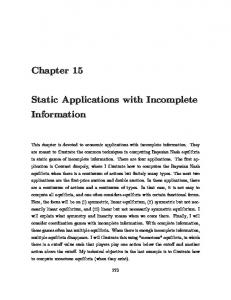
Physical problem Reading: Ch. 1 in the text

“Simple” mathematical model

• analytical solution • F.E. solution(s)

More complex mathematical model • holes included • large disp./large strains • F.E. solution(s) ⇒ • How many finite elements? We need a good error measure (especially for FSI) “Even more complex” mathematical model

The “complex mathematical model” includes Fluid Structure Interaction (FSI).

You will use ADINA in your projects (and homework) for structures and fluid flow. 3

MIT 2.094

1.2

1. Large displacement analysis of solids/structures

Large Displacement analysis

Lagrangian formulations: • Total Lagrangian formulation • Updated Lagrangian formulation

1.2.1

Reading: Ch. 6

Mathematical model/problem

Given

Calculate

the the the the the

original configuration of the body, support conditions, applied external loads, assumed stress-strain law deformations, strains, stresses of the body.

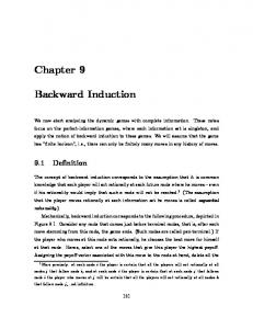
Question Is there a unique solution? Yes, for infinitesimal small displacement/strain. Not necessarily for large displacement/strain. For example: Snap-through problem

The same load. Two different deformed configurations. 4

MIT 2.094


Column problem, statics

Not physical

1.2.2

t

R is in “direction” of bending moment ⇒ Not in equilibrium.

Requirements to be fulfilled by solution at time t

I. Equilibrium of stresses (Cauchy stresses, forces per unit area in t V and on t Sf ) with the applied body forces t f B and surface tractions t f Sf II. Compatibility III. Stress-strain law

1.2.3

Finite Element Method

I. Equilibrium condition means now • equilibrium at the nodes of the mesh • equilibrium of each finite element II. Compatibility satisfied exactly III. Stress-strain law satisfied exactly

5

MIT 2.094

1.2.4


Notation

Cauchy stresses (force per unit area at time t):

t

τij

i, j = 1, 2, 3

t

τij = t τji

(1.1)

6


Fall ‘08

Lecture 2 - Finite element formulation of solids and structures Prof. K.J. Bathe

MIT OpenCourseWare

Assume that on t Su the displacements are zero (and t Su is constant). Need to satisfy at time t: • Equilibrium of Cauchy stresses t τij with applied loads � � t T τ = t τ11 t τ22 t τ33 t τ12 t τ23 t τ31

(2.1)

(For i = 1, 2, 3)

t

τij,j + t fiB t

=

t

τij nj

=

t Sf fi

=

(e.g.

0 in t V (sum over j)

(2.2)

t Sf fi on t Sf (sum over j) t τi1 t n1 + t τi2 t n2 + t τi3 t n3

(2.3)

)

(2.4)

S

And: t τ11 t n1 + t τ12 t n2 = t f1 f

• Compatibility The displacements t ui need to be continuous and zero on t Su . • Stress-Strain law t

� � τij = function t uj

(2.5)

7

Reading: Ch. 1, Sec. 6.1-6.2

MIT 2.094

2. Finite element formulation of solids and structures

Principle of Virtual Work∗

2.1

�

t

τij t eij d t V =

�

tV

tV

t B fi

ui d t V +

� tS

t Sf fi

S

u i f d t Sf

(2.6)

f

where t eij � � with ui � t

=

1 2

�

∂ui ∂uj + t ∂ t xj ∂ xi

� (2.7)

= 0

(2.8)

Su

2.2

Example

Assume “plane sections remain plane” Principle of Virtual Work � � t t τ11 t e11 d V = tV

tV

t B f1

t

�

t

u1 d V + tS

S

Pr u 1 f d t S f

(2.9)

f

Derivation of (2.9) t

�t ∗ or

τ11,1 + t f1B = 0 � τ11,1 + t f1B u1 = 0

by (2.2)

(2.10) (2.11)

Principle of Virtual Displacements

8

MIT 2.094

Hence, �

2. Finite element formulation of solids and structures

�t

tV

� τ11,1 + t f1B u1 d t V = 0

� tS τ11 u1 � t Sf − � �� u� t

�

t

tV

S

u1 f tτ11 tSf

t

(2.12)

�

u1,1 τ d V + �� 11

tV

u1 t f1B d t V = 0

(2.13)

te11

where tτ11 | tS = tPr . f

Therefore we have � � t t e τ d V = t 11 11 tV

S

u1 t f1B d t V + u1 f t Pr t Sf

tV

(2.14)

From (2.12) to (2.14) we simply used mathematics. Hence, if (2.2) and (2.3) are satisfied, then (2.14) must hold. If (2.14) holds, then also (2.2) and (2.3) hold! Namely, from (2.14) � � � tS u1,1 tτ11 d tV = u1 tτ11 � tSf − u

tV

tV

u1 tτ11,1 d tV =

�

tV

S

u1 tf1B d tV + u1 f tPr tSf

(2.15)

or � u1 tV

�t � � S � τ11,1 + tf1B d tV + u1 f tPr − tτ11 tSf = 0

� Now let u1 = x 1 −

x tL

��

(2.16)

� τ11,1 + tf1B , where tL = length of bar.

t

Hence we must have from (2.16) t

τ11,1 + tf1B = 0

(2.17)

and then also t

Pr = tτ11

(2.18)

9


Fall ‘08

Lecture 3 - Finite element formulation for solids and structures Prof. K.J. Bathe

MIT OpenCourseWare

Reading: Sec. 6.1-6.2

We need to satisfy at time t: • Equilibrium ∂ tτij t B + fi = 0 ∂ txj t

(i = 1, 2, 3) in t V

t Sf

τij tnj = fi

(3.1)

(i = 1, 2, 3) on t Sf

(3.2)

• Compatibility • Stress-strain law(s) Principle of virtual displacements � � � t τij teij d tV = ui tfiB d tV + tV

1 teij = 2

tV

�

∂ ui ∂uj + t ∂ t xj ∂ xi

tS f

ui | t S

f

t Sf fi

d tSf

(3.3)

� (3.4)

• If (3.3) holds for any continuous virtual displacement (zero on tSu ), then (3.1) and (3.2) hold and vice versa.

• Refer to Ex. 4.2 in the textbook.

10

MIT 2.094

3. Finite element formulation for solids and structures

Major steps I. Take (3.1) and weigh with ui : �t � τij,j + t fiB ui = 0.

(3.5a)

II. Integrate (3.5a) over volume t V : � �t � τij,j + t fiB ui d t V = 0

(3.5b)

tV

III. Use divergence theorem. Obtain a boundary term of stresses times virtual displacements on t S = t Su ∪ t Sf . IV. But, on t Su the ui = 0 and on t Sf we have (3.2) to satisfy. Result: (3.3). Example

�

t tV

τ11 te11 d tV =

�

t S

tS f

ui f1 f d tSf

(3.6)

One element solution:

11

MIT 2.094


1 1 (1 + r) u1 + (1 − r) u2 2 2 1 1 t t u(r) = (1 + r) u1 + (1 − r) t u2 2 2 1 1 u(r) = (1 + r) u1 + (1 − r) u2 2 2 u(r) =

(3.7) (3.8) (3.9)

Suppose we know t τ11 , t V , t Sf , t u ... use (3.6). For element 1, t e11

� tV

∂u = t = B (1) ∂ x

�

u1 u2

for el. (1) T t −→ te11t τ11 d V

� (3.10)

� [u1

u2 ] tV

� for el. (1)

−→ ⎡

= ⎣ U1 �� u2

B (1)

T

t

τ11 d t V ��

(3.11)

= t F (1)

u2 ] t F (1) ⎤ � t (1) � Fˆ U 2 U 3⎦ �� 0

[u1

(3.12) (3.13)

u1

where t

(1) (1) Fˆ1 = t F2

t ˆ (1) F2

=

(3.14)

t (1) F1

(3.15)

For element 2, similarly, ⎡ ⎤ = ⎣U 1

U2 �� u2

U3 ⎦ ��

�

0 t ˆ (2) F

� (3.16)

u1

R.H.S. ⎡

�

U1

�

U2 �� U

T

U3

⎤ (unknown reaction at left) ⎣ ⎦ 0 t Sf � t Sf · f 1

�

(3.17)

Now apply, U

T

=

�

1

0 0

�

(3.18)

=

�

0

1 0

�

(3.19)

=

�

0

0 1

�

(3.20)

then, U

T

then, U

T

12

MIT 2.094


This gives, ⎡

�

t

Fˆ (1) 0

�

� +

t

0 ˆ F (2)

�

⎤ unknown reaction ⎢ ⎥ 0 =⎣ ⎦ t tSf t f1 · Sf

(3.21)

We write that as t

F = tR � � t F = fn t U1 , t U2 , t U3

(3.22) (3.23)

13


Fall ‘08

Lecture 4 - Finite element formulation for solids and structures Prof. K.J. Bathe

MIT OpenCourseWare

We considered a general 3D body,

Reading: Ch. 4

The exact solution of the mathematical model must satisfy the conditions: • Equilibrium within t V and on t Sf ,

• Compatibility

• Stress-strain law(s) I. Differential formulation II. Variational formulation (Principle of virtual displacements) (or weak formulation) We developed the governing F.E. equations for a sheet or bar

We obtained t

F = tR

(4.1)

where t F is a function of displacements/stresses/material law; and t R is a function of time. Assume for now linear analysis: Equilibrium within 0 V and on 0 Sf , linear stress-strain law and small displacements yields t

F = K · tU

(4.2)

We want to establish, KU (t) = R(t)

(4.3) 14

MIT 2.094


Consider

ˆT = U

�

U1

V1

W1

U2

· · · WN

�

(N nodes)

(4.4)

ˆ T is a distinct nodal point displacement vector. where U Note: for the moment “remove Su ” We also say � ˆ T = U1 U

U2

U3

· · · Un

�

(n = 3N )

(4.5)

We now assume ⎤(m) u = ⎣ v ⎦ w ⎡

ˆ, u(m) = H (m) U

u(m)

(4.6a)

ˆ is n x 1. where H (m) is 3 x n and U ˆ �(m) = B (m) U

(4.6b)

where B (m) is 6 x n, and T

�(m) = e.g. γxy

�

�xx �yy ∂v ∂u

= + ∂x ∂y

�zz

γxy

γyz

γzx

�

We also assume u(m) �

(m)

=

ˆ H (m) U

(4.6c)

=

(m)

ˆ U

(4.6d)

B

15

MIT 2.094


Principle of Virtual Work: � � T T ˆ f B dV

� τ dV = U V

(4.7)

V

(4.7) can be rewritten as �� m

T

�(m) τ (m) dV (m) =

��

V (m)

m

ˆ U

(m) T

fB

(m)

dV (m)

(4.8)

V (m)

Substitute (4.6a) to (4.6d). � � � � T (m) T (m) (m) ˆ U B τ dV =

V (m)

m

ˆ U

T

� ��

H

(m) T

f

B (m)

(4.9)

� dV

(m)

V (m)

m

ˆ τ (m) = C (m) �(m) = C (m) B (m) U

Finally, � �� T � ˆ U �

B

(m) T

(4.10)

� C

(m)

B

(m)

dV

(m)

ˆ = U

V (m)

m

� �� T � ˆ U � m

H

(m) T

(4.11)

� fB

(m)

dV (m)

V (m)

with T

T

ˆ B (m) �(m) = U

T

(4.12)

ˆ = RB KU

(4.13)

where K is n x n, and RB is n x 1. Direct stiffness method: � K= K (m)

(4.14)

m

RB =

�

(m)

RB

(4.15)

m

K

(m)

(m)

RB

�

T

B (m) C (m) B (m) dV (m)

= �V

(m)

V

(m)

T

H (m) f B

=

(m)

(4.16)

dV (m)

(4.17)

16

MIT 2.094


Example 4.5 textbook

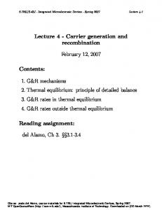
E = Young’s Modulus

Mathematical model

Plane sections remain plane:

F.E. model

⎡

⎤ U1 U = ⎣ U2 ⎦ U3

(4.18)

Element 1

⎡

u(1) (x) =

� �

1−

x 100

x

�� 100

H (1)

⎤

U1

0 ⎣ U2 ⎦ � U 3 �

(4.19)

17

MIT 2.094


⎤ U1 0 ⎣ U2 ⎦ � U 3

(4.20)

x 80

(4.21)

⎡

�(1) xx (x) =

�

1 − 100

�

1

��100

B (1)

�

Element 2 u(2) (x) =

�

0

� �(2) xx (x)

=

� �

0

x 1 − 80 ��

H (2) 1 1 − 80 80

��

B (2)

�

U

� �

U

(4.22)

�

Then, ⎡ ⎤ 1 −1 0 0 13E ⎣ E ⎣ −1 1 0 ⎦ + 0 K= 240 100 0 0 0 0 ⎡

⎤ 0 0 1 −1 ⎦ −1 1

(4.23)

where,

� � A�

< η=0

1

� � AE E(1) ≡ L 100 � � 13 E E · 13 = 3 80 3 · 80 � �� A∗ � � A∗ < A�

(4.24) (4.25)

(4.26)

η=80

< 4.333
0 for w ∈ V

� 0) (w =

2x (strain energy when imposing w)

Also, a(wh , wh ) > 0 for wh ∈ Vh

(Vh ⊂ V, wh �= 0)

31

Reading: Sec. 5.5.5, 4.3

MIT 2.094 Property I

7. Isoparametric elements Define: eh = u − uh .

From (7.22), a(u, vh ) = (f , vh )

(7.24)

From (7.23), a(uh , vh ) = (f , vh )

(7.25)

Hence, a(u − uh , vh ) = 0

(7.26)

a(eh , vh ) = 0

(7.27)

(error is orthogonal in that sense to all vh in F.E. space). Property II a(uh , uh ) ≤ a(u, u)

(7.28)

Proof: a(u, u) = a(uh + eh , uh + eh )

(7.29)

� 0 by Prop. I �� 2a(u = a(uh , uh ) + � �� h , eh )

+ a(eh , eh ) � ��

(7.30)

≥0

∴ a(u, u) ≥ a(uh , uh )

(7.31)

32


Fall ‘08

Lecture 8 - Convergence of displacement-based FEM Prof. K.J. Bathe

MIT OpenCourseWare

(A) Find u ∈ V such that a(u, v) = (f , v) ∀v ∈ V (Mathematical model)

(8.1)

a(v, v) > 0 ∀v ∈ V,

(8.2)

v= � 0.

where (8.2) implies that structures are supported properly. E.g.

(B) F.E. Problem

Find

uh ∈ Vh such that a(uh , vh ) = (f , vh ) ∀vh ∈ Vh

a(vh , vh ) > 0

∀vh ∈ Vh ,

vh �= 0

(8.3)

(8.4)

Properties eh = u − uh (I) a(eh , vh ) = 0

∀vh ∈ Vh

(8.5)

(II) a(uh , uh ) ≤ a(u, u)

(8.6)

33

MIT 2.094

8. Convergence of displacement-based FEM

� � (C) Assume Mesh�

� � e.g. Mesh�

h1

h1

� � “is contained in” Mesh�

� � not contained in Mesh�

h2

h2

We assume (C), but need another property (independent of (C))

(III) a(eh , eh ) ≤ a(u − vh , u − vh ) ∀vh ∈ Vh

(8.7)

uh minimizes! (Recall eh = u − uh ) Proof: Pick wh ∈ Vh . �0 �� a(eh + wh , eh + wh ) = a(eh , eh ) + � 2a(e + a(wh , wh ) �� h , wh ) � ��

(8.8)

≥0

Equality holds for (wh = 0)

a(eh , eh ) ≤ a(eh + wh , eh + wh ) = a(u − uh + wh , u − uh + wh )

(8.9) (8.10)

Take wh = uh − vh . a(eh , eh ) ≤ a(u − vh , u − vh )

(8.11)

Using property (III) and (C), we can say that we will converge monotonically, from below, to a(u, u): 34

MIT 2.094


Pascal triangle (2D)

⇒ 4-node element is complete to k = 1. ⇒ 9-node element is complete to k = 2.

(Ch. 4.3)

error in displacement ∼ C · hk+1

(8.12)

(C is a constant determined by the exact solution, material property. . . ) error in stresses ∼ C · hk

error in strain energy ∼ C · h2k

(8.13)

(← these C are different)

(8.14)

Hence, E − Eh = C · h2k

(roughly equal to)

(8.15)

By theory, log (E − Eh ) = log C + 2k log h

(8.16)

35

MIT 2.094


By experiment, we can evaluate log(E − Eh ) for different meshes and plot log(E − Eh ) vs. log h

We need to use graded meshes if we have high stress gradients. Example

Consider an almost incompressible material:

�V = vol. strain

(8.17)

� · v → very small or zero

(8.18)

or

We can “see” difficulties: p = −κ�V

κ = bulk modulus

(8.19)

As the material becomes incompressible (ν = 0.3 → 0.4999) � κ→∞ p → finite number �V → 0

(8.20)

(Small error in �V results in huge error on pressure as κ → ∞, the constant C in (8.15) can be very large ⇒ locking)

36


Fall ‘08

Lecture 9 - u/p formulation Prof. K.J. Bathe

MIT OpenCourseWare

We want to solve

Reading: Sec. 4.4.3

I. Equilibrium � τij,j + fiB = 0 in Volume S τij nj = fi f on Sf

(9.1)

II. Compatibility III. Stress-strain law Use the principle of virtual displacements � �T C� dV = R

(9.2)

V

We recognize that if ν → 0.5 �V → 0

(�V = �xx + �yy + �zz ) E →∞ κ= 3(1 − 2ν) p = −κ�V must be accurately computed

(9.3) (9.4) (9.5)

Solution τij = κ�V δij + 2G��ij

(9.6)

where � 1 δij = Kronecker delta = 0

i=j i= � j

(9.7)

Deviatoric strains: �V ��ij = �ij − δij 3 τij = −pδij + 2G��ij

(9.8)

�

p=−

τkk � 3

(9.9)

(9.2) becomes � � �T � � � C � dV + �V κ�V dV = R V V � � T �� C � �� dV − �TV p dV = R V

(9.10) (9.11)

V

37

MIT 2.094

9. u/p formulation

We need another equation because we now have another unknown p.

p + κ�V = 0

(9.12)

p (p + κ�V ) dV = 0 �V � p� − p �V + dV = 0 κ V

(9.13)

�

(9.14)

For an element, ˆ u = Hu � ˆ � = BD u ˆ �V = BV u

(9.16) (9.17)

p = Hp pˆ

(9.18)

(9.15)

Plane strain (�zz = 0) 4/1 element

Example

�V = �xx + �yy ⎡ �xx − 31 (�xx + �yy ) ⎢ �yy − 1 (�xx + �yy ) 3 �� = ⎢ ⎣ γxy − 13 (�xx + �yy )

Reading: Ex. 4.32 in the text

(9.19) ⎤ ⎥ ⎥ ⎦

(9.20)

� 0! Note: �zz = 0 but ��zz =

p = Hp pˆ = [1]{p0 }

(9.21)

p(x, y) = p0

(9.22)

We obtain from (9.11) and (9.14) � �� ˆ Kuu Kup u R = Kpu Kpp pˆ 0

(9.23)

�

T � BD C BD dV V

� =− BVT Hp dV V � =− HpT BV dV V � 1 =− HpT Hp dV κ V

Kuu =

(9.24a)

Kup

(9.24b)

Kpu Kpp

(9.24c) (9.24d)

38

MIT 2.094

9. u/p formulation

In practice, we use elements that use pressure interpolations per element, not continuous between elements. For example:

Then, unless ν = 0.5 (where Kpp = 0), we can use static condensation on the pressure dof’s. ˆ equations. Use pˆ equations to eliminate pˆ from the u � � −1 ˆ=R Kuu − Kup Kpp Kpu u

(9.25)

(In practice, ν can be 0.499999. . . ) The “best element” is the 9/3 element. (9 nodes for displacement and 3 pressure dof’s). p(x, y) = p0 + p1 x + p2 y

(9.26)

The inf-sup condition

Reading: Sec. 4.5

⎡

⎤ =�V � �� ⎢ ⎥ ⎢ Vol qh � · vh dVol ⎥ inf sup ⎢ ⎥≥β>0 �� ⎣ �qh � �vh � ⎦ � �� qh ∈Qh vh ∈Vh

(9.27)

for normalization

Qh : pressure space. If “this” holds, the element is optimal for the displacement assumption used (ellipticity must also be satisfied). Note: infimum = largest lower bound

supremum = least upper bound

For example, inf {1, 2, 4} = 1

sup {1, 2, 4} = 4

inf {x ∈ R; 0 < x < 2} = 0

sup {x ∈ R; 0 < x < 2} = 2

(9.23) rewritten (κ = ∞, full incompressibility). Diagonalize using eigenvalues/eigenvectors. For a mesh of element size h we want βh > 0 as we refine the mesh, h → 0

39

MIT 2.094

9. u/p formulation

For

(entry [3,1] in matrix) assume the circled entry is the minimum (inf) of

.

Also, all entries in the matrix not shown are zero. Case 1 βh = 0 ⎧ 0 · uh |i = 0 (from the bottom equation) ⎨ ⇒ α · u | + 0 · ph |j = Rh |i (from the top equation) ⎩ �� h i � =0

⇒ no equation for ph |j ⇒ spurious pressure! (any pressure satisfies equation) Case 2 βh = small = � � · uh |i = 0 ∴�·

⇒ uh |i = 0

ph |j + uh |i · α = Rh |i Rh |i

⇒ ph |j = �

� ⇒

displ. = pressure →

0 large

�

as � is small

The behavior of given mesh when bulk modulus increases: locking, large pressures. See Example 4.39 textbook.

40


Fall ‘08

Lecture 10 - F.E. large deformation/general nonlinear analysis Prof. K.J. Bathe

MIT OpenCourseWare

We developed � t τij teij d tV = tR

Reading: Ch. 6

(10.1)

tV

1 teij = 2

�

�

∂ui ∂uj + t ∂ txj ∂ xi

� (10.2)

τij δt eij d tV = tR

t tV

1 δt eij = 2

�

∂(δui ) ∂(δuj ) + ∂ t xj ∂ t xi

(10.3)

� (≡ t eij )

(10.4)

In FEA: t

F = tR

(10.5)

In linear analysis t

F = K t U ⇒ KU = R

(10.6)

In general nonlinear analysis, we need to iterate. Assume the solution is known “at time t” t

x=

0

x + tu

(10.7)

Hence t F is known. Then we consider t+Δt

F =

t+Δt

R

(10.8)

Consider the loads (applied external loads) to be deformation-independent, e.g.

41

MIT 2.094

10. F.E. large deformation/general nonlinear analysis

Then we can write t+Δt

F = tF + F

(10.9)

t+Δt

U = tU + U

(10.10)

where only t F and t U are known.

F ∼ = tK ΔU ,

t

K = tangent stiffness matrix at time t

(10.11)

From (10.8), t

K ΔU =

t+Δt

R − tF

(10.12)

We use this to obtain an approximation to U . We obtain a more accurate solution for U (i.e. using t+Δt

K (i−1) ΔU (i) = t+Δt

U

(i)

=

t+Δt

R − t+ΔtF (i−1)

t+Δt

U

(i−1)

+ ΔU

t+Δt

F)

(10.13)

(i)

(10.14)

Also, t+Δt

F (0) = tF

t+Δt

K

(0)

(10.15)

t

= K

(10.16)

U (0) = tU

(10.17)

t+Δt

Iterate for i = 1, 2, 3 . . . until convergence. Convergence is reached when � � � � �ΔU (i) � < �D � �2 � t+Δt t+Δt (i−1) � R− F � � < �F 2

Note: �a�2 =

��

2

(ai )

i

�

ΔU

(i)

=U

i=1,2,3...

ΔU (1) in (10.13) is ΔU in (10.12).

(10.13) is the full Newton-Raphson iteration.

How we could (in principle) calculate t K

Process • Increase the displacement t Ui by �, with no increment for all t Uj , j �= i • calculate

t+�

F

• the i-th column in tK = ( t+�F − tF ) /� =

∂ tF . ∂ tUi

42

(10.18) (10.19)

MIT 2.094


So, perform Pictorially, ⎡ .. ⎢ . ⎢ t K = ⎢ ... ⎣ .. .

this process for i = 1, 2, 3, . . . , n, where n is the total number of degrees of freedom. .. . .. . ··· .. .

⎤ ⎥ ⎥ ⎥ ⎦

A general difficulty: we cannot “simply” increment Cauchy stresses. •

t+Δt

τij referred to area at time t + Δt

• t τij referred to area at time t. We define a new stress measure, 2nd Piola - Kirchhoff stress, refers to original configuration. Then, t+Δt 0 Sij

= 0tSij + 0 Sij

t+Δt 0 Sij ,

where 0 in the leading subscript (10.20)

The strain measure energy-conjugate to the 2nd P-K stress 0tSij is the Green-Lagrange strain 0t�ij Then, � 0V

t 0 Sij

Also, � 0V

δ 0t�ij d 0V = tR

t+Δt 0 Sij

δ t+Δt0�ij d 0V =

(10.21)

t+Δt

R

(10.22)

Example

43

MIT 2.094


t

F = tR

t+Δt

F =

(10.23)

t+Δt

R

(10.24)

(every time it is in equilibrium) (10.13) and (10.14) give: i = 1, t+Δt

K (0) ΔU (1) = t+Δt

R − t+ΔtF (0) ≡ fn( tU )

=

t+Δt

K (1) ΔU (2) =

t+Δt

U

(1)

t+Δt

(10.25)

(1)

(10.26)

R − t+ΔtF (1)

(10.27)

U

(0)

+ ΔU

i = 2, t+Δt

t+Δt

U

(2)

=

t+Δt

U

(1)

+ ΔU

(2)

(10.28)

44


Fall ‘08

Lecture 11 - Deformation, strain and stress tensors Prof. K.J. Bathe

MIT OpenCourseWare

We stated that we use � � t t τij δ teij d V = tV

Reading: Ch. 6 t 0 Sij

0V

δ 0t�ij d 0V = tR

(11.1)

The deformation gradient We use txi = 0xi + tui ⎤ ⎡ ∂ tx ∂ tx ∂ tx 1

⎢ ⎢ ⎢ t ⎢ X = 0 ⎢ ⎢ ⎣

1

1

∂ 0x1

∂ 0x2

∂ 0x3

t

t

t

∂ x2 ∂ 0x1

∂ x2 ∂ 0x2

∂ x2 ∂ 0x3

∂ tx3 ∂ 0x1

∂ tx3 ∂ 0x2

∂ tx3 ∂ 0x3

⎥ ⎥ ⎥ ⎥ ⎥ ⎥ ⎦

(11.2)

⎤ d tx1 d tx = ⎣ d tx2 ⎦ d tx3 ⎡ 0 ⎤ d x1 d 0x = ⎣ d 0x2 ⎦ d 0x3 ⎡

(11.3)

(11.4)

Implies that d tx = 0tX d 0x

(11.5)

(0tX is frequently denoted by 0tF or simply F , but we use F for force vector) We will also use the right Cauchy-Green deformation tensor t 0C

= 0tX T 0tX

Some applications

45

(11.6)

MIT 2.094

11. Deformation, strain and stress tensors

The stretch of a fiber ( tλ): � t �2 � t �2 d txT d tx ds λ = 0 T 0 = 0 d x d x d s

(11.7)

The length of a fiber is � �1 d 0s = d 0xT d 0x 2

(11.8)

� 0 T t T��t � 0 � t �2 d x 0X 0X d x λ = , d 0s · d 0s

from (11.5)

(11.9)

Express � � d 0x = d 0s 0n

(11.10)

0

0

n = unit vector into direction of d x � t �2 0 T t 0 ⇒ λ = n 0 C n

∴ tλ =

(11.11) (11.12)

� 0 T t 0 � 12 n 0C n

(11.13)

Also, �

ˆ d tx

�T � t � � t � � t � · d x = d sˆ d s cos tθ,

From (11.5), �

ˆT ˆ T 0tX d 0x

cos tθ =

��

t 0X

d 0x

d tsˆ d ts 0 0ˆT t 0 d sˆ n 0 C n d 0s = d tsˆ · d ts

∴ cos tθ =

(a · b = �a��b� cos θ)

(11.14)

� �

t ˆ 0X

≡ 0tX

�

(11.15) (11.16)

0ˆT t 0 n 0C n tλ ˆ tλ

(11.17)

Also, 0 t

ρ=

ρ

det 0tX

(see Ex. 6.5)

(11.18)

Example

Reading: Ex. 6.6 in the text

46

MIT 2.094


1 (1 + 0x1 )(1 + 0x2 ) 4

h1 =

(11.19)

.. . t

xi = 0xi + tui =

4 �

hk txki ,

(11.20) (i = 1, 2)

(11.21)

k=1

where txki are the nodal point coordinates at time t ( tx11 = 2, tx12 = 1.5) Then we obtain � 1 5 + 0x2 t 1 0X = 4 2 (1 + 0x2 ) At 0x1 = 0, 0x2 = 0, � � 1 5 � t = 0 X �0 4 12 xi = 0x2 =0

1 + 0x1 1 0 2 (9 + x1 )

1

� (11.22)

� (11.23)

9 2

The Green-Lagrange Strain t 0�

=

� 1 �t � 1 �t T t 0X 0X − I = 0C − I 2 2

∂ ∂ txi = ∂ 0xj

(11.24)

�0 � xi + tui ∂ tui = δ + ij ∂ 0xj ∂ 0xj

We find that

�

1 �t t t t t 0�ij = 0ui,j + 0uj,i + 0uk,i 0uk,j , 2

(11.25)

sum over k = 1, 2, 3

(11.26)

where t 0ui,j

=

∂ tui ∂ 0xj

(11.27)

47

MIT 2.094


Polar decomposition of 0tX t 0X

= 0tR 0tU

(11.28)

where 0tR is a rotation matrix, such that t T t 0R 0R

=I

(11.29)

and 0tU is a symmetric matrix (stretch)

Ex. 6.9 textbook

� t 0X

=

√ 3 2 1 2

1 − √2 3 2

��

4 3

0

0

� (11.30)

3 2

Then, � �2 = 0tX T 0tX = 0tU � 1 �� t �2 t −I 0� = 0U 2

t 0C

(11.31) (11.32)

This shows, by an example, that the components of the Green-Lagrange strain are independent of a rigid-body rotation.

48


Fall ‘08

Lecture 12 - Total Lagrangian formulation Prof. K.J. Bathe We discussed: �

MIT OpenCourseWare

�

t 0X

∂ txi = ∂ 0xj

t 0C

= 0tX T 0tX

⇒

d tx = 0tX d 0x,

d 0x =

(12.1) (12.2)

�

d 0x = 0t X d tx

� t �−1 t dx 0X

where 0t X =

0

� t �−1 ∂ xi = 0X ∂ txj

The Green-Lagrange strain: � 1 �t � 1 �t T t t 0� = 0X 0X − I = 0C − I 2 2

� (12.3)

(12.4)

Polar decomposition: t 0X

= 0tR0tU ⇒ 0t� =

� 1 �� t � 2 −I 0U 2

(12.5)

We see, physically that:

where d t+Δtx and d tx are the same lengths ⇒ the components of the G-L strain do not change.

Note in FEA � ⎫ 0 xi = hk 0xki ⎪ ⎪ ⎬ k for an element � t ⎪ ui = hk tuki ⎪ ⎭

(12.6)

k

t

xi = 0xi + tui →

for any particle

(12.7)

Hence for the element � � t xi = hk 0xki + hk tuki k

=

�

(12.8)

k

hk

�0 k t k� xi + ui

(12.9)

k

=

�

hk txkk

(12.10)

k

49

MIT 2.094

12. Total Lagrangian formulation

E.g., k = 4

2nd Piola-Kirchhoff stress 0 t 0S

Then � 0V

=

ρ0 t 0 T X τ tX tρ t

t 0 Sij

→

δ 0t�ij d 0V =

� tV

components also independent of a rigid body rotation

(12.11)

t

(12.12)

τij δ t eij d tV = tR

We can use an incremental decomposition of stress/strain.

t+Δt 0S t+Δt 0 Sij t+Δt

0� t+Δt 0�ij

= 0tS + 0 S

(12.13)

= 0tSij + 0 Sij

(12.14)

= =

t 0� + 0� t 0�ij + 0�ij

(12.15) (12.16)

Assume the solution is kown at time t, calculate the solution at time t + Δt. Hence, we apply (12.12) at time t + Δt: � t+Δt t+Δt 0 t+Δt R (12.17) 0 Sij δ 0�ij d V = 0V

Look at δ 0t�ij : � 1 �t t t t 0ui,j + 0uj,i + 0uk,i 0uk,j 2� � 1 ∂δui ∂δuj ∂δuk ∂ tuk ∂ tuk ∂δuk t δ 0�ij = + 0 + 0 · 0 + 0 · 0 2 ∂ 0xj ∂ xi ∂ xi ∂ xj ∂ xi ∂ xj � � 1 δ 0t�ij = δ 0ui,j + δ 0uj,i + δ 0uk,i 0tuk,j + 0tuk,i δ 0uk,j 2 δ 0t�ij = δ

(12.18a) (12.18b) (12.18c)

We have t+Δt 0�ij

− 0t�ij = 0�ij 0�ij

(12.19)

= 0eij + 0 ηij

(12.20)

50

MIT 2.094


where 0eij is the linear incremental strain, 0 ηij is the nonlinear incremental strain, and ⎛ 0eij

=

⎞

1⎜ ⎟ t t ⎝ u + u + u u + u u ⎠ 2 0 i,j 0 j,i �0 k,i 0 k,j �� 0 k,i 0 k,j�

(12.21)

initial displ. effect

1 u u 0 ηij = 2 0 k,i 0 k,j

(12.22)

where 0uk,j

=

∂uk , ∂ 0xj

uk =

t+Δt

uk − tuk

(12.23)

Note δ t+Δt�ij = δ 0�ij

�

� δ 0t�ij = 0 when changing the configuration at t + Δt

�

(12.24)

From (12.17): � �t �� δ 0eij + δ 0 ηij d 0V 0 Sij + 0 Sij 0V

� = 0V

=

�t � 0 t 0 Sij δ 0eij + 0 Sij δ 0eij + 0 Sij δ 0 ηij + 0 Sij δ 0 ηij d V

(12.25)

t+Δt

R

Linearization ⎛ ⎞ t t 0 KN L U 0 KL U � ⎜� �� t �� ⎟ 0 ⎜0 Sij δ 0eij + 0 Sij δ 0 ηij ⎟ d V = ⎝ ⎠

(12.26)

t+Δt

�

R−

0V

0V

�

t 0 0 Sij δ 0eij d V

��

t 0F

(12.27)

�

We use, 0 Sij

� 0 Cijrs 0ers

(12.28)

We arrive at, with the finite element interpolations, �t � t t+Δt R − 0tF 0 KL + 0 KN L U = where U is the nodal displacement increment.

51

(12.29)

MIT 2.094


Left hand side as before but using (k − 1) and right hand side is � t+Δt (k−1) 0 t+Δt = t+ΔtR − d V 0 Sij δ 0�ij

(12.30)

0V

gives t+Δt

R−

t+Δt (k−1) 0F

In the full N-R iteration, we use � � t+Δt (k−1) t+Δt (k−1) + ΔU (k) = 0 KL 0 KN L

(12.31)

t+Δt

R−

52

t+Δt (k−1) 0F

(12.32)


Fall ‘08

Lecture 13 - Total Lagrangian formulation, cont’d Prof. K.J. Bathe

MIT OpenCourseWare

Example truss element. Recall:

Principle of virtual displacements applied at some time t + Δt:

�

t+Δt

τij δ t+Δteij d t+ΔtV =

t+ΔtV

� 0V

t+Δt 0 Sij t+Δt 0�ij 0�ij

t+Δt t+Δt 0 0 Sij δ 0�ij δ V

=

t+Δt

(13.1)

t+Δt

(13.2)

R R

= 0tSij + 0 Sij =

t 0�ij

(13.3)

+ 0�ij

(13.4)

= 0eij + 0 ηij

(13.5)

where 0tSij and 0t�ij are known, but 0 Sij and 0�ij are not. � 1� t t 0ui,j + 0uj,i + 0uk,i 0uk,j + 0uk,j 0uk,i 2 � 1� 0 ηij = 0uk,i 0uk,j 2 0eij

=

Substitute into (13.2) and linearize to obtain � � t 0 δ 0eij 0 Cijrs 0ers d 0V + 0 Sij δ 0 ηij d V = 0V

F.E. discretization gives �t � t 0 KL + 0 KN L ΔU =

(13.6) (13.7)

t+Δt

0V

t+Δt

R − 0tF

�

R− 0V

δ 0eij 0tSij d 0V

(13.8)

(13.9)

53

MIT 2.094

13. Total Lagrangian formulation, cont’d

�

t 0 KL

=

t 0 KN L

=

0V

� 0V

t T t 0 0 BL 0 C 0 BL d V

(13.10)

t T 0 BN L

(13.11)

t t 0 0 S 0 BN L d V ��

matrix

�

t 0F

= 0V

t T 0 BL

tˆ 0 0S d V ��

(13.12)

vector

The iteration (full Newton-Raphson) is � � t+Δt (i−1) t+Δt (i−1) + ΔU (i) = 0 KL 0 KN L

t+Δt

U (i) =

t+Δt

R−

t+Δt

U (i−1) + ΔU (i)

Truss element example

t+Δt (i−1) 0F

(13.13)

(13.14)

(p. 545)

Here we have to only deal with 0tS11 , 0e11 , 0 η11 0e11 0 η11

∂u1 ∂ tu ∂uk + 0 k · 0 0 ∂ x1 ∂ x1 ∂ x1 � � 1 ∂uk ∂uk = · 2 ∂ 0x1 ∂ 0x1 =

(13.15) (13.16)

We are after ⎞ u11 ⎜ u12 ⎟ t ⎟ ˆ = 0tBL ⎜ ⎝ u21 ⎠ = 0 BL u u22 ⎛

0e11

ui =

2 �

(13.17)

hk uki

(13.18)

k=1

t

ui =

2

�

hk tuki

(13.19)

k=1

54

MIT 2.094


∂u1 ∂ tu1 ∂u1 ∂ tu2 ∂u2 + + ∂ 0x ∂ 0x1 ∂ 0x1 ∂ 0x1 ∂ 0x1 �0 1 � t 2 0 u1 = L + ΔL cos θ − L � � t 2 u2 = 0L + ΔL sin θ

0e11

0e11

=

1 � −1 =0 L ⎛

0 1

�

0

(13.20a) (13.20b) (13.20c)

ˆ u ⎞

⎜ ⎟ ⎜0 ⎟ ⎜ L + ΔL ⎟ 1 � ⎟· +⎜ cos θ − 1 ⎜ ⎟ 0L −1 0L ⎜� �� ⎟ ⎝ ⎠

0

1

�

0

ˆ u

∂ tu1 ∂ 0x1

⎛

⎞

⎜ ⎟ ⎜0 ⎟ ⎜ L + ΔL ⎟ 1 � ⎜ +⎜ sin θ⎟ ⎟ · 0L 0 0L ⎜� ⎟ �� ⎝ ⎠

−1

0

1

�

ˆ u

(13.20d)

∂ tu2 ∂ 0x1

ˆ =0tBL u

(13.20e)

Hence, 0 0e11

=

L + ΔL �

− cos θ

2 ( 0L)

− sin θ

cos θ

sin θ

�

ˆ u

(13.20f)

where the boxed quantity above equals 0tBL . In small strain but large rotation analysis we assume ΔL � 0L, 0e11

=

0 η11

δ 0 η11

1 �

− cos θ

0L

1 = 2

�

− sin θ

cos θ

∂u1 ∂u1 ∂u2 ∂u2 + 0 0 0 ∂ x1 ∂ x1 ∂ x1 ∂ 0x1

sin θ

�

ˆ u

(13.20g)

� (13.21a)

� � 1 ∂δu1 ∂u1 ∂u1 ∂δu1 ∂δu2 ∂u2 ∂u2 ∂δu2 = + 0 + 0 + 0 2 ∂ 0x1 ∂ 0x1 ∂ x1 ∂ 0x1 ∂ x1 ∂ 0x1 ∂ x1 ∂ 0x1 � � ∂δu1 ∂u1 ∂δu2 ∂u2 = + 0 ∂ 0x1 ∂ 0x1 ∂ x1 ∂ 0x1

t 0 S11 δ 0 η11

=

�

∂δu1 ∂ 0x1

∂δu2 ∂ 0x1

�� tS 0 0 11 t 0 0 S11 � ��

∂u1 ∂ 0x1 ∂u2 ∂ 0x1

(13.21b) (13.21c)

� (13.21d)

t 0S

�

∂u1 ∂ 0x1 ∂u2 ∂ 0x1

� =

1 0L �

�

−1 0

0 −1 ��

BN L

1 0 0 1

� ˆ u

(13.21e)

� 55

MIT 2.094

0C tˆ 0S


=E

(13.22)

= 0tS11

(13.23)

Assume small strains t 0K

EA 0L ⎡ cos2 θ ⎢ =⎢ ⎣ sym � =

⎡

cos θ sin θ sin2 θ

1 P ⎢ 0 ⎢ +0 ⎣ −1 L 0 � t

− cos2 θ − sin θ cos θ cos2 θ ��

t 0 KL

0 −1 0 1 0 1 −1 0 ��

t 0 KN L

⎤ − cos θ sin θ − sin2 θ ⎥ ⎥ sin θ cos θ ⎦ sin2 θ �

⎤ 0 −1 ⎥ ⎥ 0 ⎦ 1 �

When θ = 0, 0tKL doesn’t give stiffness corresponding to u22 , but 0tKN L does.

56

(13.24)


Fall ‘08

Lecture 14 - Total Lagrangian formulation, cont’d Prof. K.J. Bathe

MIT OpenCourseWare

Truss element. 2D and 3D solids.

�

t+Δt

τij δ t+Δteij d t+ΔtV =

t+ΔtV

� 0V

� 0V

0 Cijrs 0ers δ 0eij δ

t+Δt t+Δt 0 0 Sij δ 0�ij δ V

(14.1)

t+Δt

(14.2)

R R

⏐ ⏐ � linearization

�

t 0 t+Δt R− 0 Sij δ 0 ηij δ V =

�

0

=

t+Δt

V + 0V

0V

t 0 0 Sij δ 0eij δ V

(14.3)

Note: δ 0eij = δ 0t�ij varying with respect to the configuration at time t. F.E. discretization � 0 xi = hk 0xki

t

xi =

k t

ui =

�

�

t+Δt

hk txki

xi =

k

hk tuki

t+Δt

ui =

k

(14.4) into (14.3) gives �t � t 0 KL + 0 KN L U =

�

�

hk t+Δtxki

(14.4a)

hk uik

(14.4b)

k

hk t+Δtuik

k

ui =

� k

t+Δt

R − 0tF

(14.5)

57

MIT 2.094


Truss

ΔL 0L

� 1 small strain assumption: t 0K

=

E 0A 0L ⎡

⎢ =⎢ ⎣

+

cos2 θ cos θ sin θ − cos2 θ 2 cos θ sin θ sin θ − sin θ cos θ cos2 θ − cos2 θ − cos θ sin θ 2 − cos θ sin θ − sin θ sin θ cos θ ⎡ ⎤ 1 0 −1 0 t ⎥ P ⎢ 0 0 1 −1 ⎢ ⎥ 0L ⎣ −1 0 1 0 ⎦ 0 1 0 −1

⎤ − cos θ sin θ − sin2 θ ⎥ ⎥ sin θ cos θ ⎦ sin2 θ

(14.6)

(notice that the both matrices are symmetric)

�

u1 v1

�

� =

cos θ − sin θ

sin θ cos θ

��

�

u1 v1

(14.7)

Corresponding to the u and v displacements we have: t 0K

=

=

E 0A 0L ⎡

1 ⎢ 0 ⎢ ⎣ −1 0

(14.8) 0 0 0 0

⎤

−1 0 0 0 ⎥ ⎥+ 1 0 ⎦ 0 0

⎡ t

P

0L

1 ⎢ 0 ⎢ ⎣ −1 0

⎤

0 −1 0 0 −1 ⎥ 1 ⎥ 0 1 0 ⎦ −1 0 1

58

(14.9)

MIT 2.094


t

Q 0L = tP · Δ

⇒

P

Q=

0L

· Δ

(14.10) t

where the boxed term is the stiffness. In axial direction, 0

E A 0L

�

t

P

0L

t

. But, in vertical direction,

P

0L

P

0L

is not very important because usually

is important.

⎡

⎤ − cos θ

⎥

⎢ t t ⎢ − sin θ ⎥ 0 F = P ⎣ cos θ ⎦ sin θ 2D/3D (e.g. Table 6.5)

(14.11)

2D:

�2 � �2 � 1 �� t t � u + u = u + u u + u u + 0 2,1 0 11 0 1,1 0 1,1 0 1,1 0 2,1 0 2,1 0 1,1 � �� 2� �� 0e11

(14.12)

0 η11

0�22

= · · ·

(14.13)

0�12

= · · ·

(14.14)

= ?

(14.15)

(Axisymmetric) 0�33

� 1 �� t � 2 −I 0U 2⎡ ⎤ × × 0 ⎣ × × 0 ⎦ t 2 0 0 × 0U = ↑ t 2 ( λ) t 0�

=

� � 2π 0x1 + tu1 d ts λ= 0 = d s 2π 0x1 t u =1+ 0 1 x1

(14.16)

(14.17)

t

t 0�33

� �2 u1 1+ 0 − 1

x1

� �2 t u 1 tu1 = 0 1 + x1 2 0x1

1 = 2

��

(14.18)

t

(14.19)

59

MIT 2.094


t+Δt 0�33

0�33 =

t

u + u1 1 = 10 + x1 2

t+Δt 0�33

− 0t�33 =

�t �2 u 1 + u1 0x 1

t u 1 u1 1 u1 0x + 0x · 0x + 2 1 1 1

(14.20)

�

�2 u1 0x 1

(14.21)

How do we assess the accuracy of an analysis? • Mathematical model ∼ u • F.E. solution ∼ uh

Find �u − uh � and �τ − τh �.

References [1] T. Sussman and K. J. Bathe. “Studies of Finite Element Procedures - on Mesh Selection.” Computers & Structures, 21:257–264, 1985. [2] T. Sussman and K. J. Bathe. “Studies of Finite Element Procedures - Stress Band Plots and the Evaluation of Finite Element Meshes.” Journal of Engineering Computations, 3:178–191, 1986.

60

Reading: Sec. 4.3.6


Fall ‘08

Lecture 15 - Field problems Prof. K.J. Bathe

MIT OpenCourseWare

Heat transfer, incompressible/inviscid/irrotational flow, seepage flow, etc.

Reading: Sec. 7.2-7.3

• Differential formulation • Variational formulation • Incremental formulation • F.E. discretization

15.1

Heat transfer

Assume V constant for now: S = Sθ ∪ Sq

θ(x, y, z, t) is unkown except θ|Sθ = θpr . In addition, q s |Sq is also prescribed.

15.1.1

Differential formulation

I. Heat flow equilibrium in V and on Sq . ∂θ II. Constitutive laws qx = −k ∂x .

∂θ qy = −k ∂y

∂θ

qz = −k ∂z

(15.1) (15.2)

III. Compatibility: temperatures need to be continuous and satisfy the boundary conditions. 61

MIT 2.094

15. Field problems

Heat flow equilibrium gives � � � � � � ∂ ∂θ ∂ ∂θ ∂ ∂θ k + k + k = −q B ∂x ∂x ∂y ∂y ∂z ∂z

(15.3)

where q B is the heat generated per unit volume. Recall 1D case:

unit cross-section dV = dx · (1)

(15.4)

q |x − q |x+dx + q B dx = 0 � ∂qx q|x − q|x + dx + q B dx = 0 ∂x

(15.5)

�

−

�

∂ ∂x

∂ ∂x

−k

� k

∂θ ∂x

∂θ ∂x

�

�

(15.6)

� + qB � �=0 dx dx �

(15.7)

= −q B

(15.8)

We also need to satisfy ∂θ = qS ∂n

k

(15.9)

on Sq .

15.1.2 � θ

Principle of virtual temperatures ∂ ∂x

�

∂θ k ∂x

� + ··· + q

B

� =0

(15.10)

� ( θ�S = 0 and θ to be continuous.) θ

�

� θ V

∂ ∂x

� � � ∂θ k + · · · + q B dV = 0 ∂x

(15.11) 62

MIT 2.094

15. Field problems

Transform using divergence theorem (see Ex 4.2, 7.1) � � � �T Sq � B θ kθ dV = θq dV + θ q S dSq �� V

V

heat flow

⎛

∂θ ∂x

⎞

⎜ ⎜ θ =⎜ ⎜ ⎝

∂θ ∂y

⎟ ⎟ ⎟ ⎟ ⎠

�

(15.12)

Sq

(15.13)

∂θ ∂z

⎡

k k=⎣ 0 0

0 k 0

⎤ 0 0 ⎦ k

(15.14)

Convection boundary condition � � qS = h θe − θS

(15.15)

where θe is the given environmental temperature. Radiation � � �4 � 4 q S = κ∗ (θr ) − θS � � �2 � � r �� 2 = κ∗ (θr ) + θS θ + θS θr − θS � � = κ θr − θS

(15.16) (15.17) (15.18)

where κ = κ(θS ) and θr is given temperature of source. At time t + Δt � � � � T t+Δt t+Δt � S t+Δt B θ k θ dV = θ q dV + θ t+Δtq S dSq V

V

t+Δt

θ = tθ + θ

Let

t+Δt (i)

or

θ

t+Δt (0)

with

θ

=

t+Δt (i−1)

θ

(15.19)

Sq

(15.20) + Δθ

(i)

(15.21)

t

= θ

(15.22)

From (15.19) � �T (i) θ t+Δtk(i−1) Δθ � dV V � � �T t+Δt � (i−1) = θ t+Δtq B dV − θ t+Δtk(i−1) θ dV V V � � �� (i−1) (i) S + θ t+Δth(i−1) t+Δtθ e − t+Δtθ S + ΔθS dSq

(15.23)

Sq

where the ΔθS

(i)

term would be moved to the left-hand side.

We considered the convection conditions � � � S θ t+Δth t+Δtθ e − t+Δtθ S dSq

(15.24)

Sq

The radiation conditions would be included similarly.

63

MIT 2.094

15. Field problems

F.E. discretization θ = H1x4 · t+Δtθˆ4x1 t+Δt � θ2x1 = B2x4 · t+Δtθˆ4x1 t+Δt S θ = H S · t+Δtθˆ t+Δt

for 4-node 2D planar element

(15.25) (15.26) (15.27)

For (15.23) �

⎛ ⎞ � gives (i) θ t+Δtk(i−1) Δθ � dV =⇒ ⎝ �� B T t+Δtk(i−1) �� B dV ⎠ Δ �� θˆ(i) � �� V �T

V

�

4x2

θ t+Δtq B dV ⇒

V

�

2x4

2x2

(15.28)

4x1

H T t+Δtq B dV

(15.29)

V

� θ

� T t+Δt (i−1) t+Δt � (i−1)

k

θ

�� dV ⇒

V

B T t+Δtk(i−1) BdV

�

V

� θ

S T t+Δt (i−1)

h

�

t+Δt e

θ −

�

t+Δt S (i−1)

θ

t+Δt ˆ(i−1)

�

+ ΔθS

(i)

��

dSq

θ ��

known

(15.30)

�

=⇒

Sq

⎛ � Sq

15.2

⎛

⎞⎞

(15.31)

S T t+Δt (i−1) h H S ⎝ t+Δtθê − ⎝ t+Δtθˆ(i−1) +Δ �� H θˆ(i) ⎠⎠ dSq � �� 4x1

1x4

4x1

4x1

4x1

Inviscid, incompressible, irrotational flow

2D case: vx , vy are velocities in x and y directions. �·v =0 ∂vx ∂vy + =0 ∂x ∂y ∂vx ∂vy − =0 ∂y ∂x

or

Reading: Sec. 7.3.2

(15.32) (incompressible)

(15.33)

(irrotational)

(15.34)

Use the potential φ(x, y), vx =

⇒

∂φ ∂x

vy =

∂φ ∂y

(15.35)

∂2φ ∂2φ + 2 = 0 in V ∂x2 ∂y

(15.36)

(Same as the heat transfer equation with k = 1, q B = 0)

64


Fall ‘08

Lecture 16 - F.E. analysis of Navier-Stokes fluids Prof. K.J. Bathe

MIT OpenCourseWare

Incompressible flow with heat transfer Reading: Sec. 7.1-7.4, Table 7.3

We recall heat transfer for a solid:

Governing differential equations (kθ,i ),i + q B = 0

in V

(16.1)

� � θ�

� ∂θ �� = qS � ∂n Sq Sq

(16.2)

is prescribed, k Sθ

Sθ ∪ Sq = S

Sθ ∩ Sq = ∅

(16.3)

Principle of virtual temperatures � � � S B θ,i kθ,i dV = θq dV + θ q S dSq V

V

(16.4)

Sq

for arbitrary continuous θ(x1 , x2 , x3 ) zero on Sθ For a fluid, we use the Eulerian formulation.

65

MIT 2.094

16. F.E. analysis of Navier-Stokes fluids

� � ∂ (ρcp vθ)dx + conduction + etc ρcp v θ|x − ρcp v θ|x + ∂x

(16.5)

In general 3D, we have an additional term for the left hand side of (16.1): �� ·� v )θ − ρcp (v · �) θ −� · (ρcp vθ) = −ρcp � · (vθ) = −ρcp (� � ��

(16.6)

term (A)

where � · v = 0 in the incompressible case.

� · v = vi,i = div(v) = 0

(16.7)

So (16.1) becomes � � (kθ,i ),i + q B = ρcp θ,i vi ⇒ (kθ,i ),i + q B − ρcp θ,i vi = 0 Principle of virtual temperatures is now (use (16.4)) � � � � θ,i kθ,i dV + θ (ρcp θ,i vi ) dV = θq B dV + V

V

V

(16.8)

S

θ q S dSq

(16.9)

Sq

Navier-Stokes equations • Differential form τij,j + fiB = ρvi,j vj

(16.10)

with ρvi,j vj like term (A) in (16.6) = ρ(v · �)v in V . � � ∂vj 1 ∂vi τij = −pδij + 2µeij + eij = 2 ∂xj ∂xi

(16.11)

• Boundary conditions (need be modified for various flow conditions) Sf

τij nj = fi

on Sf

(16.12)

Mostly used as fn = τnn = prescribed, ft = unknown with possibly inflow conditions).

And vi prescribed on Sv , and Sv ∪ Sf = S and Sv ∩ Sf = ∅. 66

∂vn ∂n

=

∂vt ∂n

= 0 (outflow or

MIT 2.094


• Variational form � � � � v i ρvi,j vj dV + eij τij dV = v i fiB dV + V

V

V

S

S

v i f fi f dSf

(16.13)

Sf

� p� · vdV = 0

(16.14)

V

• F.E. solution We interpolate (x1 , x2 , x3 ), vi , v i , θ, θ, p, p. Good elements are

×: linear pressure ◦: biquadratic velocities (Q2 , P1 ), 9/3 element

9/4c element

Both satisfy the inf-sup condition. So in general,

Example:

For Sf e.g. τnn = 0,

∂vt = 0; ∂n

(16.15) 67

MIT 2.094 and

∂vn ∂t


is solved for. Actually, we frequently just set p = 0.

Frequently used is the 4-node element with constant pressure

It does not strictly satisfy the inf-sup condition. Or use

Reading: Sec. 7.4

3-node element with a bubble node. Satisfies inf-sup condition

1D case of heat transfer with fluid flow, v = constant

Re =

vL ν

Pe =

vL α

α=

k ρcp

Reading: Sec. 7.4.3

(16.16)

• Differential equations

θ|x=0 = θL

kθ�� = ρcp θ� v

(16.17)

θ|x=L = θR

(16.18)

In non-dimensional form 1 �� θ = θ� Pe

Reading: p. 683

(now θ�� and θ� are non-dimensional)

� � exp Pe θ − θL L x −1 ⇒ = θR − θL exp (Pe) − 1

(16.19)

(16.20)

68

MIT 2.094


• F.E. discretization θ�� = Peθ�

1

�

(16.21)

�

� �

1

θ θ dx + Pe 0

θθ� dx = 0 + { effect of boundary conditions = 0 here}

(16.22)

0

Using 2-node elements gives

1 2

(h∗ )

Pe =

(θi+1 − 2θi + θi−1 ) =

Pe (θi+1 − θi−1 ) 2h∗

vL α

(16.23)

(16.24)

Define Pee = Pe ·

�

h vh = L α

Pee −1 − 2

�

(16.25)

� θi−1 + 2θi +

� Pee − 1 θi+1 = 0 2

(16.26)

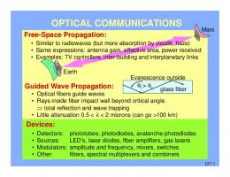
what is happening when Pee is large? Assume two 2-node elements only. θi−1 = 0 θi+1 = 1 1 θi = 2

(16.27) (16.28) � � Pee 1− 2

(16.29)

69

MIT 2.094


θi =

1 2

� 1−

Pee 2

� (16.30)

For Pee > 2, we have negative θi (unreasonable).

70


Fall ‘08

Lecture 17 - Incompressible fluid flow and heat transfer, cont’d Prof. K.J. Bathe

17.1

MIT OpenCourseWare

Abstract body Reading: Sec. 7.4

Fluid Flow Sv , Sf Sv ∪ Sf = S Sv ∩ Sf = 0

17.2

Heat transfer Sθ , Sq Sθ ∪ Sq = S Sθ ∩ Sq = 0

Actual 2D problem (channel flow)

71

MIT 2.094

17.3

17. Incompressible fluid flow and heat transfer, cont’d

Basic equations

P.V. velocities � � � � v i ρvi,j vj dV + τij eij dV = v i fiB dV + V

V

V

S

S

v i f fi f dSf

(17.1)

Sf

Continuity � pvi,i dV = 0

(17.2)

V

P.V. temperature � � � � θρcp θ,i vi dV + θ,i kθ,i dV = θq B dV + V

V

V

S

θ q S dS

(17.3)

Sq

F.E. solution xi =

�

hk xki

(17.4)

vi =

�

hk vik

(17.5)

θ=

�

hk θk

(17.6)

p=

�

˜ k pk h

(17.7)

⎛

⇒ F (u) = R

17.4

⎞ v

u = ⎝ p ⎠ nodal variables θ

(17.8)

Model problem

1D equation, ρcp v

dθ d2 θ =k 2 dx dx

(17.9)

(v is given, unit cross section) Non-dimensional form (Section 7.4) Pe

dθ d2 θ = 2 dx dx

(17.10) 72

MIT 2.094

Pe =


vL , α

α=

k ρcp

(17.11) θ∗ is non-dimensional � � exp PeLx − 1

θ − θL = exp (Pe) − 1 θR − θ L

(17.10) in F.E. analysis becomes � � dθ dθ dθ θPe dV + dV = 0 dx V V dx dx

(17.12)

(17.13)

Discretized by linear elements:

h∗ =

θ(ξ) =

� � ξ ξ 1 − ∗ θi−1 + ∗ θi h h

h L

(17.14)

For node i:

−θi−1 −

Pee Pee

θi−1 + 2θi − θi+1 + θi+1 = 0 2 2

(17.15)

where Pee =

vh α

� � h = Pe L

(17.16)

This result is the same as obtained by finite differences � 1 � θ�� = 2 (θi+1 − 2θi + θi−1 ) i (h∗ ) � θi+1 − θi−1 � θ� � = 2h∗ i 73

(17.17) (17.18)

MIT 2.094


Considered θi+1 = 1, θi−1 = 0. Then θi =

1 − (Pee /2) 2

(17.19)

Physically unrealistic solution when Pee > 2. For this not to happen, we should refine the mesh—a very fine mesh would be required. We use “upwinding” dθ �� θi − θi−1 � = dx i h∗

(17.20)

The result is (−1 − Pee ) θi−1 + (2 + Pee ) θi − θi+1 = 0 Very stable, e.g. � θi−1 = 0 θi+1 = 1

⇒ θi =

(17.21)

1 2 + Pee

(17.22)

Unfortunately it is not that accurate. To obtain better accuracy in the interpolation for θ, use the function � x� exp Pe L −1 (17.23) exp (Pe) − 1 The result is Pee dependent:

This implies flow-condition based interpolation. We use such interpolation functions—see references.

References [1] K.J. Bathe and H. Zhang. “A Flow-Condition-Based Interpolation Finite Element Procedure for Incompressible Fluid Flows.” Computers & Structures, 80:1267–1277, 2002. [2] H. Kohno and K.J. Bathe. “A Flow-Condition-Based Interpolation Finite Element Procedure for Triangular Grids.” International Journal for Numerical Methods in Fluids, 51:673–699, 2006.

74

MIT 2.094

17.5


FSI briefly

Lagrangian formulation for the structure/solid Arbitrary Lagrangian-Eulerian (ALE) formulation Let f be a variable of a particle (e.g. f = θ). Consider 1D � ∂f ∂f � f˙� = + v (17.24) ∂t ∂x particle where v is the particle velocity. For a mesh point, � ∂f ∂f � f ∗� = + vm ∂t ∂x mesh point

(17.25)

where vm is the mesh point velocity. Hence, � � ∂f � � f˙� = f ∗� + (v − vm ) ∂x particle mesh point

(17.26)

Use (17.26) in the momentum and energy equations and use force equilibrium and compatibility at the FSI boundary to set up the governing F.E. equations.

References [1] K.J. Bathe, H. Zhang and M.H. Wang. “Finite Element Analysis of Incompressible and Compressible Fluid Flows with Free Surfaces and Structural Interactions.” Computers & Structures, 56:193–213, 1995. [2] K.J. Bathe, H. Zhang and S. Ji. “Finite Element Analysis of Fluid Flows Fully Coupled with Structural Interactions.” Computers & Structures, 72:1–16, 1999. [3] K.J. Bathe and H. Zhang. “Finite Element Developments for General Fluid Flows with Structural Interactions.” International Journal for Numerical Methods in Engineering, 60:213–232, 2004. 75


Fall ‘08

Lecture 18 - Solution of F.E. equations Prof. K.J. Bathe

MIT OpenCourseWare

In structures,

Reading: Sec. 8.4

F (u, p) = R.

(18.1)

In heat transfer, F (θ) = Q

(18.2)

In fluid flow, F (v, p, θ) = R

(18.3)

In structures/solids F =

�

F (m) =

m

�� m

0V (m)

t (m) T t ˆ (m) 0 (m) d V 0S 0 BL

Elastic materials

Example

p. 590 textbook

76

(18.4)

MIT 2.094

18. Solution of F.E. equations

Material law

t 0 S11

˜ 0t�11 =E

(18.5)

In isotropic elasticity: ˜= E

t 0�

E (1 − ν) , (1 + ν) (1 − 2ν)

(ν = 0.3)

� 1 �� t � 2 1 = U − I ⇒ 0t�11 = 2 0 2

��

(18.6)

0

L + tu 0L

�2

�

1 −1 = 2

��

t

u 1+ 0 L

�

�2 −1

(18.7)

where 0tU is the stretch tensor. 0 t 0 S11

=

ρ0 X tτ 0X T tρ t 11 11 t 11

(18.8)

with 0 0 t X11

=

0L

L , + tu

t

⇒ 0tS11 =

L 0L

0

0 0

ρ L = tρ tL

(18.9)

� 0 �2 0 L L t τ11 = t tτ11 tL L

L ˜·1 ∴ t tτ11 = E L 2

��

t

u 1+ 0 L

(18.10)

�

�2 −1

(18.11)

� �� 2 �

t t Ã � E u u ⇒ τ11 A = P = 1+ 0 − 1 1 + 0 2 L L t

t

(18.12)

This is because of the material-law assumption (18.5) (okay for small strains . . . ) Hyperelasticity t 0W

= f (Green-Lagrange strains, material constants) � � 1 ∂0tW ∂0tW t + t 0 Sij = 2 ∂ 0t�ij ∂ 0�ji

� t �

∂ 0tSij 1 ∂ 0 Sij C = + 0 ijrs 2 ∂ 0t�rs ∂ 0t�sr 77

(18.13) (18.14) (18.15)

MIT 2.094


Plasticity

• yield criterion • flow rule • hardening rule t

�

t−Δt

τ =

t

τ +

dτ

(18.16)

t−Δt

Solution of (18.1) (similarly (18.2) and (18.3)) Newton-Raphson Find U ∗ as the zero of f (U ∗ ) f (U ∗ ) =

R − t+ΔtF � � � � � ∂f �� t+Δt (i−1) · U ∗ − t+ΔtU (i−1) + H.O.T. =f U + � ∂U t+ΔtU (i−1)

where

t+Δt

(18.17) (18.18)

U (i−1) is the value we just calculated and an approximation to U ∗ .

t+Δt

Assume t+ΔtR is independent of the displacements. � � ∂ t+ΔtF �� t+Δt t+Δt (i−1) � 0= R− F − · ΔU (i) ∂U � t+ΔtU (i−1)

(18.19)

We obtain

t+Δt

K (i−1) ΔU (i) =

t+Δt

K

(i−1)

t+Δt

R − t+ΔtF (i−1)

(18.20)

� � �� ∂ t+ΔtF �� ∂F �� = = ∂U � t+ΔtU (i−1) ∂U � t+ΔtU (i−1)

(18.21)

Physically

t+Δt

(i−1)

K11

Δ =

�

t+Δt

(i−1)

F1

� (18.22)

Δu 78

MIT 2.094


Pictorially for a single degree of freedom system

t

i = 1; t+Δt

i = 2; Convergence

K

K Δu(1) =

t+Δt

(1)

t+Δt

Δu

(2)

=

R − tF R−

(18.23)

t+Δt

F

(1)

(18.24)

Use

�ΔU (i) �2 < � �� 2 �a�2 = (ai )

(18.25) (18.26)

i

But, if incremental displacements are small in every iteration, need to also use � t+ΔtR − t+ΔtF (i−1) �2 < �R

18.1

(18.27)

Slender structures

(beams, plates, shells)

t �1 Li

(18.28)

79

MIT 2.094


Beam

e.g.

t L

=

1 100

(4-node el.)

The element does not have curvature → we have

a spurious shear strain

(9-node el.) → We do not have a shear (better) → But, still for thin structures, it has problems like ill-conditioning. ⇒ We need to use beam elements. For curved structures also spurious membrane strain can be present.

80


Fall ‘08

Lecture 19 - Slender structures Prof. K.J. Bathe

Beam analysis,

t L

MIT OpenCourseWare

� 1 (e.g.

t L

=

1 1 100 , 1000 , · · · )

Reading: Sec. 5.4, 6.5

(plane stress) � L � 0 2 J= 0 2t 1 h2 = (1 − r) (1 + s) 4 1 h3 = (1 − r) (1 − s) 4

(19.1) (19.2) (19.3)

Beam theory assumptions (Timoshenko beam theory): v2∗ = v3∗ = v2 t u3∗ = u2 + θ2 2 t ∗ u 2 = u2 − θ 2 2

⎡ B∗ = ⎢ ⎢ ⎢ ⎢ ⎣

(19.4) (19.5) (19.6)

u∗2

v2∗

u∗3

v3∗

− 41 (1 + s) L2

0

− 14 (1 − s) L2

0

0 1 4 (1

− r) 2t

1 4 (1

−

r) 2t

− 14 (1 + s) L2

− 14 (1

0 − 14 (1 − r) 2t 81

−

⎤ r) 2t

− 14 (1 − s) L2

⎥ etc ⎥ ⎥ ⎥ ⎦

(19.7)

MIT 2.094

19. Slender structures

u2 ⎡ Bbeam

⎢ = ⎢ ⎢ ··· ⎢ ⎣

− L1

v2

θ2 t 2L s

0

0 �

0 �

0 �

0

− L1

− 21 (1 − r)

⎤

∂u ∂x

⎛

⎜ ⎥ ⎜ ⎥ ⎜ ⎥∼⎜ ⎥ ⎜ ⎦ ⎜ ⎝

⎞ 0

∂v � ∂y � ∂u ∂y

+

∂v ∂x

⎟ ⎟ ⎟ ⎟ ⎟ ⎟ ⎠

(19.8)

1 (1 − r)v2

2 1 st

u(r) = (1 − r)u2 − (1 − r)θ2 2 4 v(r) =

(19.9) (19.10)

at r = −1, v(−1) = v2

(19.11)

st u(−1) = − θ2 + u2 2

(19.12)

Kinematics is

u(r) =

1 (1 − r)u2 2

(19.13)

results into �xx → �xx =

∂u 2 1 · =− ∂r L L

(19.14)

st (1 − r)θ2 4

(19.15)

u(r, s) = −

results into �xx , γxy → �xx =

γxy =

v(r) =

st 2L

∂u 2 1 · = − (1 − r) ∂s t 2

1 (1 − r)v2 2

(19.16)

(19.17)

(19.18)

results into γxy → γxy = −

82

1 L

(19.19)

MIT 2.094


For a pure bending moment, we want

1 1

− v2 − (1 − r)θ2 = 0 L 2

(19.20)

for all r! ⇒ Impossible (except for v2 = θ2 = 0) ⇒ So, the element has a spurious shear strain! Beam kinematics (Timoshenko, Reissner-Mindlin)

γ=

�

dw −β dx

1 3 I= bt 12

(19.21)

� (19.22)

Principle of virtual work �

L

EI 0

dβ dβ dx + AS G dx dx

�

L

�

0

dw −β dx

��

� � L dw − β dx = pwdx dx 0

As = kA = kbt

(19.23)

(19.24)

To calculate k � �2 � � V 1 1 2 (τa ) dA = dAs A 2G 2G s A AS

Reading: p. 400

(19.25)

where τa is the actual shear stress: � � �2 � t − y2 3 V 2 τa = · � t �2 2 A

(19.26)

2

and V is the shear force. ⇒k=

Reading: Ex. 5.23

5 6

(19.27)

83

MIT 2.094


Now interpolate

w(r) = h1 w1 + h2 w2

(19.28)

β(r) = h1 θ1 + h2 θ2

(19.29)

Revisit the simple case:

1+r w1 2 1+r β= θ1 2

w=

(19.30) (19.31)

Shearing strain γ=

1+r w1 − θ1 L 2

(19.32)

Shear strain is not zero all along the beam. But, at r = 0, we can have the shear strain = 0. θ1 w1 − can be zero L 2

(19.33)

Namely, θ1 w1 2 − = 0 for θ1 = w1 L L 2

(19.34)

84


Fall ‘08

Lecture 20 - Beams, plates, and shells Prof. K.J. Bathe

MIT OpenCourseWare

Timoshenko beam theory

The fiber moves up and rotates and its length does not change. Principle of virtual displacement � EI

L

� � � �T β β � dx + (Ak)G

0

0

L

(Linear Analysis) �

dw −β dx

�T �

� � L dw − β dx = wT pdx dx 0

(20.1)

Two-node element:

Three-node element:

For a q-node element, �T � ˆ = w1 · · · wq θ1 · · · θq u ˆ w = Hw u ˆ β = Hβ u � � Hw = h1 · · · hq 0 · · · 0 � � Hβ = 0 · · · 0 h1 · · · hq dx J= dr

(20.2) (20.3) (20.4) (20.5) (20.6) (20.7)

85

MIT 2.094

20. Beams, plates, and shells

dw ˆ = J −1 Hw,r u dx � ��

(20.8)

dβ ˆ = J −1 Hβ,r u dx � ��

(20.9)

Bw

Bβ

Hence we obtain � � 1 � EI BβT Bβ det(J )dr + (Ak)G −1

1

� T ˆ (Bw − Hβ ) (Bw − Hβ ) det(J )dr u

−1

�

1

=

HwT p det(J )dr

(20.10)

−1

ˆ=R Ku

(20.11)

K is a result of the term inside the bracket in (20.10) and R is a result of the right hand side. For the 2-node element,

w1 = θ1 = 0

(20.12)

w2 , θ2 = ?

(20.13)

γ=

1+r w2 − θ2 L 2

(20.14)

We cannot make γ equal to zero for every r (page 404, textbook). Because of this, we need to use about 200 elements to get an error of 10%. (Not good!) Recall almost or fully incompressible analysis: Principle of virtual displacements: � � �T � � � C � dV + �v (κ�v )dV = R V

(20.15)

V

u/p formulation � � T �� C � �� dV − �v pdV = R V V � �p � p + �v dV = 0 κ V

(20.16) (20.17)

But now we needed to select wisely the interpolations of u and p. We needed to satisfy the inf-sup condition � qh � · vh dVol ≥β>0 (20.18) inf sup Vol �� qh ��vh � qh ∈Qh vh ∈Vh

86

MIT 2.094


4/1 element:

We can show mathematically that this element does not satisfy inf-sup condition. But, we can also show it by giving an example of this element which violates the inf-sup condition.

v1 = �, above �

v2 = 0 ⇒ � · vh for both elements is positive and the same. Now, if I choose pressures as

qh �vh dVol = 0,

hence (20.18) is not satisfied!

(20.19)

Vol

9/3 element

satisfies inf-sup

9/4-c

satisfies inf-sup

Getting back to beams � L � � EI β βdx + (AkG) 0

�

0

L

�

� dw − β γ AS dx = R dx

(20.20)

L

� � γ AS γ − γ AS dx = 0

(20.21)

dw − β, dx

(20.22)

0

where γ=

from displacement interpolation 87

MIT 2.094


γ AS = Assumed shear strain interpolation

(20.23)

2-node element, constant shear assumption. From (20.21),

�

L

�

0

� � L dw �dx = �dx −β � γ AS γ AS � γ AS dx 0

�

+1

�

⇒− −1

⇒ γ AS =

1+r θ2 2

� ·

Reading: Sec. 4.5.7

(20.24)

L dr + w2 = γ AS · L 2

(20.25)

w2 − L2 θ2 L

(20.26)

γ AS (shear strain) is equal to the displacement-based shear strain at the middle of the beam.

Use γ AS in (20.20) to obtain a powerful element. For “our problem”, γ AS = 0

� ⇒ EI 0

L θ2 2

(20.27)

� � β β � dx = M β � x=L

(20.28)

hence

L

w2 =

�� 2 1 · L θ2 = M ⇒ EI L

⇒ θ2 =

ML , EI

w2 =

(20.29)

M L2 2EI

(20.30)

(exact solutions)

88

MIT 2.094


Plates

Reading: Fig. 5.25, p. 421

⎧ ⎪ ⎨ w = w(x, y) is the transverse displacement of the mid-surface v = −zβy (x, y) ⎪ ⎩ u = −zβx (x, y)

(20.31)

For any particle in the plate with coordinates (x, y, z), the expressions in (20.31) hold! We use w=

q �

hi wi

(20.32)

i=1

βx = − βy = +

q � i=1 q �

hi θyi

(20.33)

hi θxi

(20.34)

i=1

where q equals the number of nodes. Then the element locks in the same way as the displacement-based beam element.

89


Fall ‘08

Lecture 21 - Plates and shells Prof. K.J. Bathe

MIT OpenCourseWare

Timoshenko beam theory, and Reissner-Mindlin plate theory

For plates, and shells, w, βx , and βy as independent variables.

w = displacement of mid-surface, w(x, y)

A = area of mid-surface p = load per unit area on mid-surface w = w(x, y)

(21.1)

w(x, y, z) = w(x, y)

(21.2)

The material particles at “any z” move in the z-direction as the mid-surface.

u(x, y, z) = −βx z = −βx (x, y)z v(x, y, z) = −βy z = −βy (x, y)z

(21.3) (21.4)

∂βx ∂u = −z ∂x ∂x ∂βy ∂v = −z = ∂y ∂y � � ∂u ∂v ∂βx ∂βy = + = −z + ∂y ∂x ∂y ∂x

�xx =

(21.5)

�yy

(21.6)

γxy

∂βx ∂x

⎛ ⎞ ⎜ �xx ⎜ ⎝ �yy ⎠ = −z ⎜ ⎜ ⎜ γxy ⎝

⎞

⎛

�

∂βy ∂y ∂βx ∂y

+ �� κ

(21.7)

∂βy ∂x

⎟ ⎟ ⎟ ⎟ ⎟ ⎠

(21.8)

� 90

MIT 2.094

21. Plates and shells

∂w ∂u ∂w − βx + = ∂x ∂z ∂x ∂w ∂v ∂w − βy = + = ∂y ∂z ∂y

γxz = γyz

⎛

⎞ ⎡ 1 τxx E ⎝ τyy ⎠ = ⎣ ν 1 − ν2 τxy 0

ν 1 0

(21.9) (21.10)

0 0 1−ν 2

⎤⎛

⎞ �xx ⎦ ⎝ �yy ⎠ = C · � γxy

(21.11)

(plane stress)

�

τxz τyz

�

E = 2(1 + ν)

�

�

γxz γyz

= Gγ

(21.12)

Principle of virtual work for the plate:

� � A

+ 2t

⎡

�

�xx

�yy

γ xy

− 2t

� �

+ 2t

k A

− 2t

�

�

1 E ⎣ ν 1 − ν2 0 γ xz

γ yz

⎞ �xx ⎦ ⎝ �yy ⎠dzdA+ 1−ν γxy 2 � �� 1 0 γxz G dzdA = wpdA 0 1 γyz A ν 1 0

0 0

⎤⎛

(21.13)

Consider a flat element:

⎛ ⎜ ⎜ ⇒ Kb ⎜ ⎝

w1 θx1 θy1 . ..

⎞

⎛

⎟ ⎟ ⎟ , also Kpl. ⎠

where Kb is 12x12 and Kpl.

str.

⎞

u1

⎜ v ⎟ str. ⎝ 1 ⎠ ...

(21.14)

is 8x8.

91

MIT 2.094

21. Plates and shells

For a flat element: ⎛

� ⇒

Kb 0

0 Kpl. str.

⎜ ⎜ ⎜ ⎜ ⎜ �⎜ ⎜ ⎜ ⎜ ⎜ ⎜ ⎜ ⎜ ⎜ ⎝

w1 θx1 θy1 .. .

⎞

⎟ ⎟ ⎟ ⎟ ⎟ ⎟ ⎟ 4 ⎟ θy ⎟ = · · · u1 ⎟ ⎟ v1 ⎟ ⎟ .. ⎟ . ⎠ v4

(21.15)

u=

�

hi u i

(21.16)

v=

�

hi vi

(21.17)

w=

�

hi wi � βx = − hi θyi � βy = hi θxi

(21.18) (21.19) (21.20)

From (21.13) ⎡ 1 3 Et ⎣ ν κT 12 (1 − ν 2 ) A 0

�

ν 1 0

0 0 1−ν 2

⎤ � ⎦ κdA +

γ T Gt · k

A

�

1 0

0 1

� γdA

(21.21)

where k is the shear correction factor. Next, evaluate

∂w ∂w ∂βx ∂x , ∂y , ∂x ,

. . . etc. ⇒ This element, as it is, locks!

This displacement-based element “locks in shear”. We need to change the transverse shear interpola tions.

γyz =

1 1 A C (1 − r)γyz + (1 + r)γyz 2 2

(21.22)

where A γyz =

�

�� ∂w − βy �� ∂y evaluated at A

(21.23)

from the w, βy displacement interpolations. 1 1 B D (1 − s)γxz + (1 + s)γxz (21.24) 2 2 with this mixed interpolation, the element works. Called MITC interpolation (for mixed interpolatedtensional components) γxz =

92

MIT 2.094

21. Plates and shells Aside: Why not just neglect transverse shears, as in Kirchhoff plate theory? βx = 0 ⇒ βx = ∂w ∂x � 2 � • Therefore we have ∂∂xw2 , · · · in strains, so we need continuity also for � ∂w � ∂x · · · • If we do, γxz =

∂w ∂x −

• w=

� � 1 1 r(1 + r)w1 − r(1 − r)w2 + 1 − r2 w3 2 2

w2 and w3 never affect w1 (∴ w|r=1 = w1 ).

But,

∂w 1 1 = (1 + 2r)w1 − (1 − 2r)w2 − 2rw3 ∂r 2 2 � � w2 and w3 affect ∂w ∂r 1 . ⇒ This results in difficulties to develop a good element based on Kirchhoff theory.

With Reissner-Mindlin theory, we independently interpolate rotations such that this problem does not arise. For flat structures, we can superimpose the plate bending and plane stress element stiffness. For shells, curved structures, we need to develop/use curved elements, see references.

References [1] E. Dvorkin and K.J. Bathe. “A Continuum Mechanics Based Four-Node Shell Element for General Nonlinear Analysis.” Engineering Computations, 1:77–88, 1984. [2] K.J. Bathe and E. Dvorkin. “A Four-Node Plate Bending Element Based on Mindlin/Reissner Plate Theory and a Mixed Interpolation.” International Journal for Numerical Methods in Engineering, 21:367–383, 1985. [3] K.J. Bathe, A. Iosilevich and D. Chapelle. “An Evaluation of the MITC Shell Elements.” Computers & Structures, 75:1–30, 2000. [4] D. Chapelle and K.J. Bathe. The Finite Element Analysis of Shells – Fundamentals. Springer, 2003.

93

MIT OpenCourseWare http://ocw.mit.edu

2.094 Finite Element Analysis of Solids and Fluids II Spring 2011

For information about citing these materials or our Terms of Use, visit: http://ocw.mit.edu/terms.