models the 1 â αi (αi) portion of the total reward is lost at the departure from ... yi(t, w, a) + ri(1 â αi). â. âa yi(t, w, a) = qiiyi(t, w, a). (1) with initial conditions:.
Completion Time in Markov Reward Models with Partial Incremental Loss G. Horv´ath M. Telek Budapest University of Technology and Economics Dept. of Telecommunication Abstract The completion time analysis of Markov reward models with partial incremental loss is provided in this paper. The complexity of the model behaviour requires the use of an extra (supplementary) variable.
1
Introduction
The analytical description of Markov reward models (MRMs) without reward loss at state transitions is provided in [4, 3]. Based on this analytical description effective numerical methods were developed for the performance analysis of computer and communication systems [2, 5]. In this paper we consider the case when a portion of the reward accumulated during the sojourn in a state is lost at the departure of that state [1, 6].
2
Model Definition
Let the (right continuous) “structure state process”, {Z(t), t ≥ 0}, be an irreducible homogeneous continuous time Markov chain (CTMC) on state space S = {1, 2, ..., N } with generator Q = {qij } and initial probability vector γ. The amount of accumulated reward at time t is denoted by B(t). During the sojourn dB(t) = ri . in state i, the process accumulates reward with rate ri (ri ≥ 0), i.e., dt The subset of states with positive (zero) reward rate is denoted by S + (S 0 ). MRMs are classified based on their behaviour at state transitions (θk denotes the kth state transition). The case when the accumulated reward is maintained, B(θk+ ) = B(θk− ), is called preemptive resume. In partial loss reward models a portion of the accumulated reward is lost, B(θk+ ) < B(θk− ). In partial total loss models the 1 − αi (αi ) portion of the total reward is lost at the departure from state i: B(θk+ ) = αi B(θk− ). In partial incremental loss models the reward loss affects only the amount of reward accumulated during the sojourn in the last visited state: B(θi ) = B(θi−1 ) + αZ(θ− ) [B(θi− ) − B(θi−1 )]. This paper considers completion time i of MRMs with partial incremental loss.
1
3
Accumulated Reward
Differential equations has been used for the analytical description of reward models for a long time [7]. We apply the same approach for the analysis of Markov reward models with partial incremental loss, but in this case the model behavior in the (t, t + ∆) interval depends on both, B(t) and the amount of reward accumulated during the sojourn in the actual state. Due to this model feature we introduce a supplementary variable that corresponds to the amount of reward lost at a possible state transition at time t (A(t)): A(t) = The amount of reward that is lost if a state change happens at time t Let denote the distribution function of the accumulated reward by Yi (t, w, a): Yi (t, w, a) = P r(Z(t) = i, B(t) < w, A(t) < a), and let introduce its density function yi (t, w, v): P r(Z(t) = i, w ≤ B(t) < w + ∆, a ≤ A(t) < a + ∆) ∆→0 ∆2
yi (t, w, a) = lim
Theorem 1 yi (t, w, a) is the solution of the following partial differential equation: ∂ ∂ ∂ yi (t, w, a) + ri yi (t, w, a) + ri (1 − αi ) yi (t, w, a) = qii yi (t, w, a) ∂t ∂w ∂a with initial conditions:
(1)
1a) yi (0, w, a) = δ(w, a) γi 1b) yi (t, w, 0) =
X
w(1−α Z i )/αi
qk,j
k∈S,k6=i
1c) yi (t, 0, 0) = 0
w>0
a=0
if i ∈
1d) yi (t, 0, 0) = δ(w, a)
yk (t, w + a, a)da,
S+
X
k∈S 0
h
γk eQ
0t
i
if i ∈ S 0
ki
Proof 1 Note that the probability of a state transition in (t, t + ∆) vanishes as ∆ → 0 if A(t + ∆) > 0. The forward argument yi (t + ∆, w, a) = (1 + qii ∆)yi (t, w − ri ∆, y − ri (1 − αi )∆) results (1). The first initial condition comes from the assumption that the background process starts in state i with probability γi . The second initial condition (a = 0) covers the case when state change happened in (t, t + ∆): P r(Z(t + ∆) = i, w ≤ B(t + ∆) < w + ∆, 0 ≤ A(t + ∆) < ∆) = (1−qii ∆)P r(Z(t) = i, w−ri ∆ ≤ B(t) < w−ri ∆ + ∆, 0 ≤ A(t) < ∆−ri (1−αi )∆) +
X
qkj ∆
k∈S,k6=i w(1−αi ) αi ∆
X
P r(Z(t) = k, w + n∆ ≤ B(t) < w + (n + 1)∆, n∆ ≤ A(t) < (n + 1)∆)
n=1
2
Dividing both sides by ∆2 , taking the limit ∆ → 0 and observing that the first term tends to 0, we obtain initial condition 1b). The upper limit of the integral comes from relation yi (t, w, a) = 0 ∀a > w(1−αi ) which follows from the model definition. Initial condition 1c) indicated that B(t) is positive in state i with positive reward rate. Initial condition 1d) reflects that B(t) = 0 is only possible if the background process did not leave the subset of states with zero reward rate till t.
4
Completion Time
The completion time of a job with size B is defined as the time point when the reward accumulation process reaches level B first: C(B) = min(t : B(t) ≥ B). The distribution and the density function of the completion time are denoted by: Fi (t, B) = P (C(B) < t, Z(C(B)) = i), fi (t, B) =
Pr(t ≤ C(B) < t + ∆, Z(C(B)) = i) . ∆→0 ∆ lim
Due to the monotonicity of B(t) in preemptive resume reward models, fi (t, B) can be derived from the density of the accumulated reward yi (t, w): fi (t, B) = ri yi (t, B).
(2)
In partial loss models, B(t) is not monotone and it can cross level B many times (due to losses). The completion time corresponds to the first of these events by definition. Therefore we consider the process which stops the reward accumulation once it reached level B. The distribution and density functions of this modified process are denoted by: Vi (t, w, a) = P r(Z(t) = i, B(t) < w, A(t) < a, C(B) > t), vi (t, w, a) =
lim
∆→0
P r(Z(t) = i, w ≤ B(t) < w + ∆, a ≤ A(t) < a + ∆, C(B) > t) . ∆2
The following theorem provides the evolution of vi (t, w, a), which is very similar to yi (t, w, a): Theorem 2 vi (t, w, a) is the solution of the following partial differential equation: ∂ ∂ ∂ vi (t, w, a) + ri vi (t, w, a) + ri (1 − αi ) vi (t, w, a) = qii vi (t, w, a) ∂t ∂w ∂a for 0 < w < B, with boundary conditions: 2a) vi (0, w, a) = δ(w, a) γi 2b) vi (t, w, 0) =
X
k∈S,k6=i
qk,j
min{B−w,w(1−α i )/αi } Z
vk (t, w + a, a)da
a=0
3
(3)
if i ∈ S +
2c) vi (t, 0, 0) = 0
2d) vi (t, 0, 0) = δ(w, a)
X
k∈S 0
h
γk eQ
0t
i
if i ∈ S 0
ki
Proof 2 The proof is similar to the one of Theorem 1. The only difference between the two is that vi (t, w, a) is defined in a finite interval 0 < w < B, and initial condition 2b) is modified accordingly. The completion time is obtained like in the preemptive resume case (eq. (2)), by integrating over feasible range of the supplementary variable. Theorem 3 The density function of the completion time in MRMs with partial incremental loss is: Z B(1−αi ) vi (t, B, a)da fi (t, B) = ri 0
Proof 3 Pr(t ≤ C(B) < t + ∆, Z(C(B)) = i) ∆→0 ∆ 1 = lim (1 + qii ∆)P r(B − rj ∆ ≤ B(t) < B, Z(t) = i) ∆→0 ∆
fi (t, B) = lim
+
X
!
qki ∆P r(B − ckj ∆ ≤ B(t) < B, Z(t) = i)
k,k6=i B(1−αi )
∆ X 1 = lim (1+qii ∆) P r(B −rj ∆ ≤ B(t) < B, Z(t) = i, n∆ ≤ A(t) < (n+1)∆) ∆→0 ∆ n=0 B(1−αi ) ∆
= lim qii ∆→0
X
P r(B − rj ∆ ≤ B(t) < B, Z(t) = i, n∆ ≤ A(t) < (n+1)∆)
n=0 B(1−αi ) ∆
+ lim ri = ri
5
Z
∆→0 ∞
0
X
∆
n=0
P r(B −rj ∆ ≤ B(t) < B, Z(t) = i, n∆ ≤ A(t) < (n+1)∆) ri ∆2
vi (t, B, a)da
Numerical Example
There are N identical servers working on one task in a distributed manner. They write the result of their work onto a storage continuously. But this storage is slower than the sever, thus a portion of the results is kept into the memory until it can be written to the storage. The servers can break down with rate λ. At break down all the servers are switched off (to redistribute the job) and the content of their memory is lost. Thus, the 1 − α portion of the work done is lost; i.e., the ratio between the server speed and the speed of the storage device is α. With rate σ the servers are stopped, all failed servers are repaired. With rate ρ the system is switched on again. This system can be modeled by a Markov reward model with partial incremental loss. The Markov chain describing this system is show on Figure 1. The state numbering reflects the number of working servers. State M is the maintenance state.
4
Number of servers: Server break down rate: System inter-maintenance rate: Inverse of system maintenance time: Result generation speed: Ratio between server speed and storage: Job size:
N =5 λ=4 σ=1 ρ = 10 r=2 α = 0.5 B=1
Table 1: System parameters used in the example The reward rates ri and αi corresponding to the states are indicated on the dashed line. If there are k working servers, the reward rate is rk = k · r. α N =0.5 rN =Nr
α N−1=0.5 α N−2=0.5 rN−1=(N−1)r r N−2=(N−2)r
Nλ
(N−1) λ
N
N−1
σ
α 0=1 r 0 =0 λ
N−2
σ
σ
ρ
0
σ
M
rM =0 α M=1
Figure 1: Structure of the Markov chain The differential equation that provides the completion time has been implemented in Matlab. Figure 2 shows how the completion time distribution depends on α (i.e., the storage speed and the server speed) and on λ (i.e. server availablility). On the first figure we can see that the completion probability where the distribution jumps above zeros is the same, this is because changing α does not change the generator of the Markov chain, neither the reward rates, and the closest time to complete the job depends only on these. On the second figure the size of the probability jump differs, since the generator is changing with λ, which affects the sojourn time in state 0 (which has actually the largest reward rate in the model).
References [1] A. Bobbio, V. G. Kulkarni, and M. Telek. Partial loss in reward models. In 2nd Int. Conf. on Mathematical Methods in Reliability, pages 207–210, Bordeaux, France, July 2000.
5
0.9
1 alpha=0.25 alpha=0.5 alpha=0.75
0.8
0.8
Completion time probability
0.7 Completion time probability
lambda=2 lambda=4 lambda=6
0.9
0.6
0.5
0.4
0.3
0.2
0.7 0.6 0.5 0.4 0.3 0.2
0.1
0.1
0
0 0
0.05
0.1
0.15
0.2
0.25
0.3
0.35
0.4
0.45
0.5
0
0.05
0.1
0.15
Time
0.2
0.25
0.3
0.35
0.4
0.45
Time
Figure 2: Completion time distribution [2] E. de Souza e Silva and H.R. Gail. Performability analysis of computer systems: from model specification to solution. Performance Evaluation, 14:157– 196, 1992. [3] V.G. Kulkarni, V.F. Nicola, and K. Trivedi. On modeling the performance and reliability of multi-mode computer systems. The Journal of Systems and Software, 6:175–183, 1986. [4] J.F. Meyer. Closed form solution of performability. IEEE Transactions on Computers, C-31:648–657, 1982. [5] H. Nabli and B. Sericola. Performability analysis: a new algorithm. IEEE Transactions on Computers, 45:491–494, 1996. [6] V.F. Nicola, R. Martini, and P.F. Chimento. The completion time of a job in a failure environment and partial loss of work. In 2nd Int. Conf. on Mathematical Methods in Reliability (MMR’2000), pages 813–816, Bordeaux, France, July 2000. [7] A. Reibman, R. Smith, and K.S. Trivedi. Markov and Markov reward model transient analysis: an overview of numerical approaches. European Journal of Operational Research, 40:257–267, 1989.
6
0.5