of modern day workstations. Many papers have ... *This work was supported in part by the Naval Surface Warfare Center under contract N60921-92-C-0161 and by the National .... 1989] call the underlying mathematical model the analytical.
Discrete Event Dynamic Systems: Theory and Applications 3, (1993): 219-247 9 1993 Kluwer Academic Publishers, Boston. Manufactured in The Netherlands.
Specification Techniques for Markov Reward Models* BOUDEWIJN R. HAVERKORT University of Twente, Tele-lnformatics and Open Systems, 7500 AE Enschede, the Netherlands KISHOR S. TRIVEDI Duke University, Department of Electrical Engineering, Durham NC 27708-0291 Received September 5, 1992; Revised February 25, 1993
Abstract. Markov reward models (MRMs) are commonly used for the performance, dependability, and performability analysis of computer and communication systems. Many papers have addressed solution techniques for MRMs. Far less attentionhas been paid to the specificationof MRMs and the subsequentderivationof the underlying MRM. In this paper we only briefly address the mathematical aspects of MRMs. Instead, emphasis is put on specification techniques. In an application independent way, we distinguish seven classes of specification techniques: stochastic Petri nets, queuing networks, fault trees, production rule systems, communicating processes, specialized languages, and hybrid techniques. For these seven classes, we discuss the main principles, give examples and discuss software tools that support the use of these techniques. An overview like this has not been presented in the literature before. Finally, the paper addresses the generation of the underiying MRM from the high-level specification, and indicates important future research areas. Key Words: dependability,Markov reward models, performability,performance, specificationtechniques, stochastic Petri nets
1. I n t r o d u c t i o n Markov reward models have b e c o m e popular for the analysis of the performance, dependability, i.e., the reliability and/or availability [Laprie 1985], and performability of computer and c o m m u n i c a t i o n systems. This is due to the nice features of M R M s in general, b u t also to the increased capacity (both in terms of computational speed a n d m e m o r y size) of m o d e r n day workstations. M a n y papers have addressed the n u m e r i c a l techniques for the analysis of possibly large M R M s , both for their steady state and transient behavior. In special cases, M R M s exhibit closed-form solutions for their steady-state probabilities; however, closed-form expressions for the transient state probabilities are rare. In case explicit solutions (often called analytical solutions) are not feasible, M R M s with finite state space can b e solved numerically. ~ Apart from the use of numerical techniques, M R M s can also be solved by using discrete event simulation (DES). DES has an advantage that the M R M need not be available explicitly before the actual analysis starts. This feature is necessary w h e n dealing with infinite state
*This work was supported in part by the Naval Surface Warfare Center under contract N60921-92-C-0161 and by the National Science Foundation under grant CCR-9108114.
220
B.R. HAVERKORTAND K.S. TRIVEDI
spaces. In general, however, simulation is a computationaUy less attractive solution, although in particular application areas the use of fast simulation techniques for MRMs might work rather well, sometimes even better than numerical techniques [Conway and Goyal 1987; Goyal et al. 1992]. In this paper we do not deal with infinitely large MRMs, nor do we address simulation as a solution method. Although analytical, numerical, and simulative solution techniques are important, they are only part of the play. From an application point of view, equally important is the construction of the MRMs. For at least two reasons this is a difficult task: 1. Modern computer and communication systems are large and complex. The models of such systems are most often also large and complex. Manual construction of the MRM is therefore error prone, if not altogether infeasible. 2. The people that really need to apply the models, typically system designers, are not knowledgeable enough about the theory and the application of MRMs. They do know about the systems they design and that need to be modeled, but they typically do not know how to translate their designs into MRMs. It is for these reasons that special model specification techniques are needed that help system designers to describe their systems in such a way that the models can be understood at the level of the system designer, rather than at the Markov chain level. Besides model specification techniques, system designers need software environments that support these techniques. Such environments or tools, should allow for the easy specification of the models and for the automated generation of the underlying MRMs from the specification. A number of different approaches towards specification techniques for MRMs have been proposed. In this paper we recognize these approaches and classify software environments that support them. A number of publications surveying tools for MRM analysis in dependability and performability have recently appeared: Mulazzani and Trivedi [1986], Geist and Trivedi [1990], Johnson and Malek [1988], Haverkort and Niemegeers [1991], and Ciardo et al. [1989]. This article differs from the ones mentioned in that it discusses specification techniques for MRMs in general, without any emphasis on the possible application domain. This article is organized as follows. The mathematical background and interpretation of MRMs in various application domains is discussed in Section 2. Then, in Section 3 we introduce a number of requirements for MRM specification techniques and tools and distinguish a number of classifying criteria for these techniques. In Section 4 we elaborate on these seven classes of specification techniques in general and discuss numerous tools that support these techniques. In Section 5 we discuss an algorithm that generates underlying MRMs from the high-level specifications. In Section 6 we conclude the paper with a summary and an indication of interesting future research areas. 2. Markov Reward Models
In a related paper [Trivedi et al. 1992] we presented an extended overview of the solution techniques used for MRM analysis. In this section we only provide a short summary. In Section 2.1 we discuss the mathematical definition of Markov reward models and the
SPECIFICATIONTECHNIQUES FOR MARKOVREWARDMODELS
221
measures that can be supported by them. In Section 2.2 we discuss the interpretation of these models when they are used for performance, dependability, or performability analysis.
2.1. Mathematics o f MRMs The specification techniques that we will describe are to be used for the generation of MRMs which consist of a continuous-time Markov chain X = {Xt, t _> 0} on a finite state space Of, and a reward function r: J)( ~ IR. X is completely described by its generator matrix Q and the initial probability vector 7r = [ . . . , 7ri, . . . ]. For every state i E JY, the reward r(i) signifies the gain or the reward that will be obtained per unit of time. This type of MRM is called a rate-based MRM. 2 We distinguish four types of measures supported by MRMs: steady-state measures, transient measures, cumulative measures, the latter also being called performability measures. We address them below. Steady-state measures express the long-run gain per unit of time of the system. They are computed from the steady-state behavior of the Markov chain. Under the assumption that the steady state distribution of X equals p_ = [ . . . . Pi . . . . ] , the steady-state measure can be expressed as M = Z pir(i) . iE3f
(1)
The vector p can easily be computed from the system of equations p_Q = 0,
with ~
Pi = 1.
(2)
iE ~,~-
When the Markov chain is irreducible, p is independent of 7r. We will always assume so. Such a system of equations can be solved in a number of wa~. When it is small (less than 1000 equations), direct solution methods like Gaussian elimination are applicable. When it is larger, iterative methods like Gauss-Seidel iteration or successive over-relaxation are better suited [Krieger et al. 1990, Steward and Goyal 1985]. Transient measures (or instant-of-time measures) express the rate at which gain is received from the system at any particular time t. They are computed from the transient behavior of X: M(t) = Z
pi(t) r(i),
(3)
iEY
where p(t) = [ . . . . pi(t) . . . . ] follows from the linear system of differential equations ,/,,(~_~,t, = p(t)Q, dt -
with p(O) = ~r. -
(4)
222
B.R. HAVERKORT AND K.S. TR/VEDI
Cumulative measures express the overall gain that is received from a system over some finite time interval. They are computed when transient measures are integrated over a time interval [0, t], i.e., Y(t) =
r(Xs) ds.
(5)
When we define the vector function l(t) = fdp(u) du, the elements li(t) of l(t) signify the expected total time spent in state i during t h e t i m e interval [0, t)./(t) satisfies the system of the differential equations
dl(t) _ l(t)Q + 7r, dt
with l(0) = 0,
--
(6)
-
which is obtained by integrating (4). The expected value E[Y(t)] can now be expressed as
E[Y(t)] = ~_j r(i)li(t)
(7)
iEX
Both systems of differential equations ((4) and (6)) can be solved by integration methods like Runge-Kutta-Fehlberg (RKF-45), or by special techniques that exploit the stochastic nature of the problem, i.e., uniformization (also known as randomization or Jensen's method) [Gross and Miller 1984, Reibmen et al. 1989, Reibman and Trivedi 1988, 1989]. Finally, performability measures 3 express whether a prespecified gain y can be received from the system in some finite time interval [0, t]:
Fr(t, y) = Pr{Y(t) < y}.
(8)
Fr(t) can be computed by specialized algorithms, involving double Laplace transforms (in both the variables t and y) [Kulkarni et al. 1987, 1990, Smith et al. 1988] or Laguerre transforms [Ammar et al. 1989]. Other solution approaches are based on partial differential equations [Pattipati et al. 1993, Reibman et al. 1989] or are an adaptation of Jensen's method [Gross and Miller 1984, de Souza e Silva and Gail 1989, 1992]. For special cases, e.g., when X is acyclic, closed-form solutions can be derived [Donatiello and Iyer 1987, Goyal and Tantawi 1987].
2.2. Interpretation of MRMs Depending on the application, we can assign different meanings to states, state transitions, rates, and rewards. In case an MRM is used for the performance analysis of a system, every state signifies a particular distribution of customers over the resources in the system. State transitions take place when customers move from one resource to another, or when they leave or enter the system. The rates are then packet arrival rates or service rates. The
SPECIFICATION TECHNIQUES FOR MARKOV REWARD MODELS
223
rewards associated with every state are given by the number of customers at every resource. The steady-state measures then yield average resource occupancies which can, via Little's law, be used to calculate average waiting times. In case an MRM is used for the dependability analysis of a system, every state signifies a particular structure of the system under study: which components are operational and which are not and, in the latter case, which components are being repaired. State transitions then take place when components fail or are repaired, with rates that correspond to component failure and repair rates. In every state, the reward is either 1 or 0, depending on whether the overall system is or is not operational. These "on-off" rewards are generally directly available from the system specification. In case an MRM is used for the performability analysis of a system, the interpretation is the same as in the availability case, apart from the reward definition. When doing a performability study, it is assumed that the system under study does not exhibit a simple "on-off" behavior: it can work partially, which is for example the case with fault-tolerant multiprocessor systems. The reward r(i) then expresses the chosen index of system performance in state i. Such rewards are not readily available from a system specification. They have to be calculated separately, for instance, by multiple performance analyses, possibly using MRMs.
3. User Requirements and Classification Criteria In Section 3.1 we discuss an important user-oriented requirement that should be imposed on any high-level specification technique. Then, in Section 3.2, we discuss a number of important criteria that can be used to classify specification techniques, and in Section 3.3 we present a number of general requirements that should be imposed on tools that support specification techniques.
3.1. User-Oriented Requirements The users of a specification technique, use the technique to solve a certain design, reconfiguration, or dimensioning problem of a real system. These designers are in first instance interested in the solution of the problem itself, not in how this solution is actually derived. They should therefore not be bothered with problems or details of the underlying mathematical model when this is not absolutely needed. Preferably, system designers should describe their system in such a way that it is easy and natural for them to use, but that it includes enough information to allow for a numerical solution based on MRMs. The system designer, however, need not be aware of the underlying MRM. Berson et al. [Berson et al. 1987, Page et al. 1989] call the underlying mathematical model the analytical representation of the problem, i.e., a representation that directly can be assessed by numerical procedures. On the other hand, the description of the model that the system designer wants to use is called the modeler's representation. The modeler's representation should contain everything that is needed for the construction of the underlying MRM, including the specification of the measures of interest. This representation should then
B.R. HAVERKORTAND K.S. TRIVEDI
224
automatically be transformed into the analytical representation. The numerical results should then be transformed to a higher level, so that they can be understood in that context. This idea is reflected in Figure 1.
3.2. Classification Criteria for Specification Techniques By keeping the above requirement in mind, as well as by "common engineering sense," we can consider a number of criteria for classifying specification techniques for MRMs (it should be noted that these criteria are neither orthogonal nor mutually exclusive):
C 1. Domain-orientedness: a specification technique can be based on assumptions that are valid only in a particular application domain, rather then on more general assumptions. C2. Class of measures that can be supported: a specification technique might not be suitable for describing systems in such a way that there is support for all the measures mentioned in Section 2. In fact, quite often the requested measure may dictate the model type (or model details) to be used. For instance, if transient performance measures are desired, a Markov model will be required even if the queuing network satisfies product-form assumptions. C3. Modeling freedom: a specification technique can force its users to construct particularly structured models by imposing a large number of constraints. Although this criterion might seem to overlap with the domain-orientedness of a particular modeling technique, this is not true. Also for very general techniques, one can often speak of more or less restricted usage of the technique. C4. Structuredness: a specification technique can allow users to construct models in a structured fashion, e.g., hierarchically, or can allow its users only to construct fiat, "spaghetti-like" models. C5. Abstraction from the underlying mathematical model: to what extent is the underlying mathematical modeling technique hidden for the specification technique user. C6. Degree of completeness: an indication of how well a specification technique supports all possible MRMs.
(
system
) modeling"
"validatiy application results ]
application model I generation
evaluation state probabilities
Markov reward model
MRM solution module Figure 1.
~ modelers J representation
Analytical and modeler's representationof a systemmodel.
"~ analytical J representation
SPECIFICATIONTECHNIQUESFOR MARKOVREWARDMODELS
225
3. 3. Requirements with Respect to Tools Software tools that support the specification, generation and the solution of MRMs are complex software systems that should be constructed in conformance with "general software engineering rules." Without being complete, let us put forward a number of guidelines that have turned out to be useful in the construction of software tools. A software tool should be built in a modular fashion. This not only keeps the tool more open-ended, it also eases the maintenance of the tool. The interchange of data between modules and other interactions between modules should be made explicit. When program modules interchange data via files, these files should be human-readable. Although this may not yield the most efficient code, it does yield tools that are more efficient to build and maintain. After a tool has been implemented and tested fully, an inefficient data-exchange module operating with files, might be replaced by a fast common-variable or socket-based interface module. The requirements for the tools also account for the way the specifications should be given. A complex specification of a large system should preferably be given in a number of modules, every module describing a separate system part, and one or more modules that specify the interactions between the modules. As an example, in a performance modeling specification, the system description (the resources) can be made totally separate from the system workload description, as in the tool HIT [Beilner et al. 1989]. Interaction between the workload and the resources can then be specified by a third model part.
4. An Overview of Specification Techniques for MRMs In this section we will present seven different classes of specification techniques. As we will see, these seven different approaches score differently on criteria C1-C6. The seven approaches are: 1. 2. 3. 4. 5. 6. 7.
Stochastic Petri nets (Section 4.1) Queuing networks (Section 4.2) Fault-trees (Section 4.3) Production rule systems (Section 4.4) Communicating processes (Section 4.5) Specialized languages (Section 4.6) Hybrid techniques (Section 4.7)
In every section we describe the basic aspects of the specification technique (rifled basic approach) and indicate how it scores on the previously defined criteria C1-C6 (titled criterion satisfaction). A small example is presented to clarify the approach (titled example). Finally, we indicate software tools that have been developed to support the particular specification technique (tiffed tools). Although we have tried to classify the specification techniques along orthogonal lines, there is an occasional overlap between various classes. In Section 4.8 we indicate similarities and differences between the different classes of specification techniques.
226
B.R. HAVERKORTAND K.S. TRIVEDI
4.1. Stochastic Petri Nets Stochastic Petri nets (SPNs) have been developed as extensions to the nontimed Petri nets by Molloy [1982], Ajmone Marsan et al. [1984], and Meyer et al. [1985]. Although at first primarily used for the performance analysis of computer systems, SPNs are increasingly being used in other application areas as well.
Basic Approach. When using an SPN specification technique, one has to define a set of places P, a set of transitions T, and a set A of arcs between transitions and places or vice versa: A _ (P x T) tO (T x P). Each place can contain one or more tokens. Graphically, places are depicted as circles, transitions as bars, tokens as dots in circles, and arcs as arrows. The distribution of tokens over the places is called a marking and corresponds to the notion of state in a Markov chain. All places from which arcs go to a particular transition are called the input places of that transition. All places to which arcs go from a particular transition are called the output places of the transition. A transition is said to be enabled when all of its input places contain at least one token. If a transition is enabled it may fire. Upon firing, a transition removes one token from all of its input places and puts one token in all of its output places, possibly causing a change of marking, i.e., a change of state. The firing of transitions is assumed to take an exponentially distributed time. Given the initial marking of an SPN, all the markings as well as the transition rates can be derived, under the condition that the number of tokens in every place is bounded. Thus a Markov chain is obtained. The rewards are described as a function of the markings, i.e., at the SPN level. The rewards and the Markov chain together yield a MRM [Ciardo et al. 1989]. Various extensions have been made to the basic SPN model described above [Ajmone Marsan et al. 1984, Ciardo et al. 1989, Meyer et al. 1985]. These include arcs with multiplicity, a shorthand notation for multiple arcs between a place-transition pair, immediate transitions that take no time at all to fire (depicted as thin bars), and inhibitor arcs from places to transitions that prevent the transition to fire as long as there are tokens in the place (depicted as lines with a small circle as head). Also, more flexible firing rules have been proposed, most notably the introduction of gates in stochastic activity networks (SANs) [Meyer et al. 1985, Sanders and Meyer 1987] and guards or enabling functions in stochastic reward nets (SRNs) [Ciardo et al. 1991]. Criteria Satisfaction. SPNs can be used to construct models that can be solved for all of the measures discussed in Section 2. The modeling freedom is very large, however the structuredness of the models is moderate. Since there are very few restrictions, it is easy to construct models that are difficult to understand, although some extensions of SPN models allow for the hierarchical composition of submodels. When using SPN based modeling techniques, the user does not need detailed knowledge of the underlying MRM. In a fairly natural way, all possible MRMs can be specified. Example: A Cyclic-Server Model. Consider the SPN as given in Figure 2 which models a 2 station cyclic-server system such as a token ring (see also Ibe and Trivedi [1990]). There are two stations S 1 and $2. When station i has a packet to transmit, it places a token in
227
SPECIFICATION TECHNIQUES FOR MARKOV REWARD MODELS
$1
$2
A1
I
A2
Frt
Swl
To2
Tr2
Figure 2. A two-station cyclic server model.
place B i (busy). If not, it has a token in place I i (idle). A station can go from the idle to the busy state by the firing of transition Ai, modeling an arrival. When the single cyclic server, represented by the single token in the places To 1, Frl, To2, Fr2 (to station 1, from station 1, etc.), arrives at station i, i.e., when the token is in place Toi, two things can happen. When station i has a packet to transmit, i.e., when there is a token in place B/, this packet is transmitted via timed transition Tri (transmit). Upon firing of this transition, the token and the packet are grasped. At the end of the firing the token is shifted to place Fr i. The just transmitted packet is routed back to the place Ii. In this way, we establish a limited buffer of size 1 in the stations. If there is no packet to transmit, i.e., place B i is empty, the immediate transition Shi is not disabled, and without any timing delay, the token is transmitted from place Toi to place Fri. When in place Frg, after a switchover delay modeled by transition Sw i (switch), the token arrives at the next station. One instance of reward rates is the numbers of tokens in the buffer places. Tools. A wide variety of tools for stochastic Petri nets have been developed. We briefly discuss the most well-known tools that are based on MRMs. Great SPN, developed by Chiola et al. at the University of Torino [Chiola 1987], is a complete graphical Petri net tool which is primarily used for the performance analysis of computer and communication systems. Analysis techniques are mainly for steady-state measures. ESP, developed by Bobbio and Cumani [Bobbio 1989, Cumani 1985], is a textual SPN tool. In this tool, special emphasis is put on the use of general (phase-type) distributions instead of only exponential distributions, on other than steady-state measures and on the aggregation of stiff MRMs. METASAN, developed by Sanders and Meyer [1987, 1988] at the University of Michigan, is based on SANs. The tool includes steady-state, transient, and cumulative analysis methods. Steady-state and transient simulation are also available as solution methods. The tool UltraSAN, developed by Sanders et al. [Couvillion 1991] at the University of Arizona, is also based on the SAN concept. With UltraSAN, the input of the models is totally graphical. UltraSAN allows for a structured form of hierarchical modeling which
228
B.R. HAVERKORTAND K.S. TRIVEDI
results in lumped underlying MRMs that are substantially smaller (so-called reduced basemodels [Sanders and Meyer 1991]) than their "fiat" counterparts. Steady-state as well as transient simulation are also available as solution methods. SPNP, developed by Ciardo et al. [1989, 1991, 1992], is a C-based SPN tool which allows for a flexible definition of a class of SPN models known as stochastic reward nets. Steadystate, transient, and cumulative measures are supported. By the flexible use of C, it is possible to construct models hierarchically, that is, results of one model can be used in the analysis of another model, even in an iterative manner, so-called fixed-point analysis [Ciardo and Trivedi 1993]. TOMSPIN is a general SPN tool developed at SIEMENS AG [Lepold 1991a], for performance and dependability analysis. Steady-state and transient measures are supported. An approximate solution for hierarchically structured SPN models based on an approximate aggregation algorithm is also included. PENPET is a performability modeling tool developed by Lepold [1991b,c] at SIEMENS AG. It is a high-level tool built on top of TOMSPIN in which one SPN is used for the specification of system dependability aspects, and another for the system performance aspects. The textual tool MARCA has been developed by Stewart [1991] at North Carolina State University. Although not really an SPN tool, its modeling constructs, i.e., buckets, balls, and transitions, can easily be interpreted in an SPN context as places, tokens and transitions. Emphasis in the tool is on advanced steady-state numerical solvers. The graphical tool DSPNexpress has been developed by Lindemann at the Technical University of Berlin [Lindemann and German 1992]. The distinguishing aspect of this tool is that it allows for DSPNs, i.e., SPNs in which transitions may have deterministic timing. Under certain conditions, an embedded Markov chain can be constructed that allows one to solve for the steady-state probabilities.
4.2. Queuing Networks Queuing networks (QNs) have been used for the performance analysis of computer and communication systems [Lazowska et al. 1984, Trivedi 1982]. In that sense, queuing network are relatively domain-oriented. There has been occasional use of QNs in other domains, but then they seem less natural.
Basic Approach. With QNs one has to specify a number of resources (the queues and servers) as well as the way in which customers make use of these resources. The queues form the active elements that can serve customers in an order governed by the scheduling discipline such as FCFS, LCFS, PS, and priority scheduling. The customers travel through the QN according to routing chains. Customers may be grouped in classes. At every queue, customers belonging to a specific class request an exponentially distributed service. After service completion, the customer proceeds to the next queue along its routing chain. The state of a QN model is a vector consisting of the number of customers of each class residing at each queue. The completion of a service at a particular queue causes a state change. Under boundedness conditions (roughly speaking, the number of customers must be finite) a QN can be transformed into a Markov chain.
SPECIFICATIONTECHNIQUESFOR MARKOVREWARDMODELS
229
The reward structure is implicitly available in the state-space description. Generally, for all possible states a number of different rewards are maintained. For instance, the number of customers of each class at each queue, and the total number of customers at each queue can be used as rewards. Using these rewards, the steady state solution of the MRM gives the average number of customers (possibly class dependent) at each queue. Then, by applying Little's law other measures such as average response times and average waiting times can be computed.
Criteria Satisfaction. QNs are commonly used to evaluate the steady-state performance of computer and communication systems. If the MRM is generated, a key advantage is that transient measures are computed with equal ease. With QNs, users clearly have less modeling freedom then with SPNs. On the other hand, the structuredness of the models is higher. With QNs, it is also often possible to construct models in a hierarchical way. As with SPNs, it is possible to be totally unaware of the underlying MRM that is used for the QN model analysis. There are computer system aspects such as synchronization and parallelism that are difficult to capture with QNs, although various extensions have been proposed. The degree of completeness therefore is not as high as that of SPNs. Example. Consider a QN of a multiprogrammed time-sharing system shown in Figure 3. The terminals are represented by 20 parallel servers, 1 for every job. After leaving the Terminals, a job remains in the JobQ until there are less than four other jobs in the processing subsystem. Once in there, it queues for processing at the CPU, and for I/O at either station IO1 or IO2. After having received service in one of these I/O channels, the job is routed back to the Terminals or remains in the processing subsystem for (at least) one other processing cycle. All queues are of FCFS type. Since there are finitely many ways of distributing 20 customers over the five resources, a finite state MRM can be derived from this QN model.
Tools. Many performance analysis tools based on QNs exist. Most of them however, do not solve the QNs via an underlying MRM. Instead, they use product form algorithms or simulation. We are aware of only a few tools that actually use MRMs for the solution. The tool QNAP2, developed at INRIA by Potier and Veran [1986] and Veran and Potier [1985] is a general QN based performance analysis tool which supports simulation, (approximate) product form solutions as well as a numerical solution based on an underlying MRM. In fact, given a complete textual representation of a QN, the QNAP2 model is transformed to an intermediate model similar to the MARCA model (see Section 4.1). Only steady-state measures are computed. The performance analysis tool NUMAS, developed at the University of Dortmund by M/iller-Clostermann [1985], is a complete textual tool for Markovian queuing network analysis. As an extension, NUMAS allows the modeling of queues with server breakdowns and repairs. NUMAS thus allows for steady-state performability analysis. The graphical performance analysis tool MACOM, developed by Sczittnick, and M/illerClostermann at the University of Dortmund [1990], is mainly used for the steady-state analysis of blocking phenomena in communication networks. MACOM emphasizes advanced techniques for the steady-state analysis of large MRMs.
230
B.R. HAVERKORTAND K.S. TRIVEDI
r
Terminals
-
I
I o.95 1
'0.8'111
0.80
Figure 3. A QN model of a central server system.
4.2. Fault-trees Fault trees (FTs) primarily used for system dependability modeling.
Basic Approach. With FTs the conditions under which a system fails, are expressed as a tree structure. Subsystems and components must have stochastically independent failure behavior. The measures of interest are normally computed using combinatorial methods, that is, the system failure event is expressed as a logical function of the failure events of subsystems and components. Dependability measures of interest are then computed numerically or symbolically without using MRMs. However, one can also translate an FT into an MRM. In order to solve a straight FT this is relatively inefficient unless, more detailed information about system measures is needed or other model aspects are to be included such as dependencies between components. From the FT, one then directly derives a Markov chain. The rewards are very simple, being either 1 or 0, depending on whether the system is operational or not in a particular state. A specification technique that is very closely related to FTs are reliability block diagrams (RBDs). With RBDs a system is described as a graph (network) in which the nodes signify components. There are two special nodes, call them left (L) and right (R), that do not represent components. The boolean function that specifies whether the system is up is represented between nodes L and R as a series-parallel network: a series connection signifies an andcondition, whereas a parallel connection signifies an or-condition. The system is assumed operational as long as there exists a path from L to R.
Criteria Satisfaction. FTs are generally not used outside their original domain of application and they seem most suitable for calculating dependability measures. With FTs the modeling freedom is very much restricted. The modeling process is highly structured. FTs for a specific system can easily be embedded in an FT for another system; in this way hierarchical modeling is possible. Users of an FT-based modeling technique might be totally unaware of the underlying MRM. Since FTs do not allow for dependencies by themselves, various augmentations of FTs are needed to model realistic systems.
231
SPECIFICATION TECHNIQUES FOR MARKOV REWARD MODELS
Example. Consider a system consisting of four components: A, B1, B2, and C. For the system to operate correctly, component A, one of components B 1 or B 2, and component C need to operate correctly. Denoting by D(x) the condition that component x is down, the condition that the system is down is expressed as D(system) = D(A) or (D(B 1) and D(B2)) or D(C). In an FT representation this would be depicted as in Figure 4, where the notation X : kx means that component X fails with rate kx. A RBD representation of the same system is given in Figure 5. Given that the system has 4 components which are initially operational, ther are 24 = 16 states. From the FT, it is easy to derive the corresponding absorbing Markov chain. For every state, the reward is either 0 or 1. If we are not interested in the exact state whenever the system is down, a considerably reduced Markov chain with only four states can be constructed: three operational states (all components up, only B 1 down, only B2 down) and one down state. If components can also be repaired (an extra parameter, the repair rate/~x, should then be added for component X) then the reduced MRM cannot be used.
Tools. The graphical tool HARP has been developed by Trivedi et al. for the analysis of large reliability models [Bavuso et al. 1987]. Apart from the aforementioned logical operators (and, or), HARP also allows for the use of logical k-out-of-n operator which keeps the FTs compact. With HARP transient measures, i.e., reliabilities and instantaneous availabilities, can be calculated.
Figure 4. FT representation of a four-component system.
~7~
B1 : ABI
Figure 5, RBD representation of a four-component system.
9
232
B.R. HAVERKORTAND K.S. TRIVEDI
4.4. Production Rule Systems Production nile systems (PRS) have been used for the construction of MRMs for system performance, dependability, and performability modeling.
Basic Approach. When using a PRS, one has to define a number of state variables, together with their initial values. Then, via so-called production rules, one specifies the conditions under which the state variables may change, as well as the rate at which these state changes take place. For instance, we have the following production rule: i f Condition(ThisState) then NewState := f ( T h i s S t a t e ) w i t h
rate k(ThisState),
meaning that whenever the conditon holds in ThisState, a new state can be reached with state dependent rate of change X. The total model state generally consists of a number of state variables. A production rule can be applied to one or more state variables at a time. The conditions can be functions of more than one state variable. It is relatively easy to specify conflicting rules. Conflict-freeness should be enforced by supporting tools. A separate part of the PRS specification describes the reward assignments. Again by using expressions over the state variables, rewards can be assigned, for instance as follows: i f Condition(State) then reward := Expression1 else reward := Expression2.
In this assignment all states which fulfill the Cond i t i on are assigned the reward as given by Express ion1, else the reward given by Expression2. The expressions again can make use of the state variables. The rewards thus specified, together with the earlier specified Markov chain constitute the MRM.
Criteria Satisfaction. Basically, PRS based specification techniques are very general and not application-dependent. Furthermore, there seems to be no restriction on the type of measures that can be supported by models constructed with PRS. The modeling freedom is very large which, however, often has a negative influence on the structuredness of the models. All possible MRMs can be specified: the specification technique is complete. In principle hierarchical modeling is possible, we are however not aware of any approach which includes this possibility.4 By using suitable abstractions and state variables, the method very closely resembles SPNs.
Example. Consider a fault-tolerant system with N active components and K cold standby spares. Whenever a component fails, with rate f, it is scheduled for repair. If a spare is available, it is switched in. Spares are assumed not to fail. Whenever a component repair finishes, it either becomes active, in case the number of active components is less than N, or it joins the pool of spares, in case there are already N operational components. In Figure 6 we present a pseudocode description of this system. Three state variables are introduced: u p, d own, and s p a r e. They model the number of operational, failed and spare components. Initially, they are set to N, 0, and K respectively.
SPECIFICATION TECHNIQUES FOR MARKOVREWARDMODELS
233
declare up initial N; declare down initial O; declare
spare
initial K;
rulel: if (up>O) and (spare>O) then spare := spare - I; down := down + 1 with rate up*f; rule2: if (up>O) and (spare=O) then up := up - i; down := down + i with rate up*f; rule3: if (down>O) and then up := up + i; down with rate r;
(upO) and (up=N) then spare := spare + I; down := down - 1 with rate r; define reward av: if (up=N) then av := 1 else av := O; define reward perf: perf := up;
Figure d PRS for a repairable fault-tolerant system with standbys. The system model is specified by means of four production rules. Rule 1 states that whenever there are operational components as well as spares available, operational components might fail, with a rate proportional to their number and the per-component failure ratef. Since there are spares available, the failure of a component does not affect the number of operational components: a spare is immediately switched in. Consequently, the number of spares decreases by 1, the number of failed components increases by 1. Rules 2-4 can be interpreted in a similar way. Two reward definitions follow: The reward av (availability) equals 1 if there are N operational components, and 0 elsewhere. The reward p e r f (performability) equals the number of operational components. Tools. The textual tool METFAC, developed by Carrasco and Figueras at the University of Catalunya [Carrasco 1986, Carrasco and Figueras 1986], supports the use of a PRS specification technique and has been used for performance, dependability and performability modeling of computer systems. Steady-state, transient, as well as cumulative measures can be computed. The tool ASSIST has been developed by Johnson and Butler at NASA [1988] as a frontend to the SURE package [Butler 1986] for reliability analysis of (computer) systems. This textual tool allows for the flexible specification of PRS. By the use of arrays of state variables and loops in the production rules, compact specifications can be written. Also facilitates for truncating state spaces are available. The ASSIST program translates the PRS to input for the SURE package. This input is a pure MRM. The SURE package deals with absorbing semi-Markov models. Therefore, only transient measures are computed.
234
B.R. HAVERKORTAND K.S. TRIVEDI
The textual tool USENUM, developed by Sczittnick et al. at the University of Dortmund [Buchholz 1991, Sczittnick 1987], allows users to define Markovian models by means of a finite state machine. USENUM can be used stand-alone, or within the QN tool MACOM.
4.5. Communicating Processes Communicating processes (CPs) have been used for the construction of MRMs for various applications. The approach shows similarity with process algebraic languages like CSP [Hoare 1985] and LOTOS [van Eijk et al. 1989] and closely resembles PRSs as well.
Basic Approach. With PRSs, there is the concept of state, however, now it is distributed over a number of processes. Instead of production rules, one now specifies communication patterns between processes. All processes have internal state variables. The set of all state variables of all processes forms the overall model state. State variables can only be changed by the process they belong to. These changes, called events, occur with certain rates. Local events only affect the internal state of their process, independently of the other processes. Other events have a more global impact. For instance, they require events in other processes to occur simultaneously (synchronizing events), or they can only take place when other events in other processes have (or have not yet) occurred. In this way processes may block one another. Note that the communication patterns are purely a modeling construct. They do not cost any time, nor do they have to conform any communication pattern in the real system being modeled. Given that for each process the state variables have initial values, the activation of the processes cause state changes which in turn cause other state changes, etc. Under boundedness conditions, a finite continuous-time Markov chain is described, assuming an exponential duration of the events. Apart from this tree-search method of deriving the underlying MRM (see Section 5), a compositional approach in which the overall Markov chain is constructed from the Markov chains describing the individual processes, can also be employed (see the tool PEPS below). As in the PRS modeling techniques, rewards can be associated with all possible states. As a result, an MRM is generated.
Criteria Satisfaction. The CP method is very general and allows for the construction of MRMs that can be analyzed for all types of measures. The modeling freedom is large, as long as systems are described as a set of communicating processes. Moreover, for a large variety of application areas this seems very natural to do. With CPs, all possible MRMs can be obtained. The structuredness of the model can be a problem, however, by using "clean" programming principles easy-to-understand models can be obtained. The method requires the notion of system state to be clear as well as the explicit binding of rewards to these states, so knowledge about MRMs helps to understand the method better. Example. Consider modeling simple queuing networks by means of CPs. We do so by first specifying a single-server queue. Then we will define a queuing network, using instances of the just defined queue.
235
SPECIFICATION TECHNIQUES FOR MARKOV REWARD MODELS
We can view a single server queue as a black box which can accept jobs from the environment, i.e., it has an input gate, and that can serve jobs. After having received service, jobs are transmitted to the environment via an output gate. The internal state of a queue is given by the number of jobs it contains. Two other characteristics are the server speed and the initial number of jobs that is present. We can define such a single-server queue by the object definition in Figure 7a. An object q u e u e is defined with two parameters: i n i t, the initial number of jobs, and s p e e d , the speed of the server. Also, two gates are defined: in and o u t . The internal state of queue is given by the state variable M. Two internal processes are defined. The first process, a r r i re, unconditionally (this can be seen from the empty guard: [ ]) accepts messages mess from the i n gate. Upon such an acceptance, the internal state variable of the queue is increased by 1. The second internal process models the servicing of jobs. Given that there are jobs (the guard [M>0] must be true), the number of jobs is decreased by 1 (M:=M-1), and a message mess is sent to the out gate with rate speed. A simple closed queuing network with a maximum of N customers and two serial queues with rates/z 1 and/z 2 can now easily be defined as in Figure 7b. Two queues, Q1 and Q2 are defined, the former with service rate/x 1 and initial number of customers N, the latter with service rate/z 2 and initial number of customers 0. By the two con n e c t statements, the output of Q1 (O2) is connected to the input of Q2 (Q1). The object definition together with instantiation of real objects specifies a Markov chain model by the allowed communication patterns. Rewards for every state can be defined by expressions over the object state variables. For instance, the average number of jobs in queue Q1 and Q2 can be calculated as the steady-state reward rate of the MRM, given that the following rewards rl and r2 are used: rl:=Q1.M
and
r2:=Q2.M.
The process definition can be extended to allow for the recognition of various message contents or probabilistic routing. define object queue(init, speed)[in, out]; state variable M initial init; process arrive; []: in?"mess"; M:=M+t; end process;
declare declare connect connect
QI: queue(N, #1); q2: queue(0, ~2); ql.out to Q2.in; Q2.out to Ql.in;
process serve(speed); [M>O]: M:=M-I; out!"mess" with rate speed; end process; end object;
(a) Figure 7. CP definition of a single-server queue.
(b)
236
/3.R. HAVERKORT AND K.S. TRIVEDI
Tools. The object-oriented tool TANGRAM has been developed by Berson et al. at the University of California at Los Angeles [Berson et al. 1987, Page et al. 1989, de Souza e Silva and Gail 1992]. With TANGRAM, communicating processes are represented by communicating objects. The object-orientation has as an advantage that object families can be defined and these can be used to compose hierarchical models. Also, inheritance of objects eases the specification of large models. The rewards are specified in a query-like fashion. It is relatively easy to tailor TANGRAM to a specific application domain or to another specification technique. For example, TANGRAM has been tailored successfully to SPN and QN like techniques as well as to the "specialized languages" technique SAVE. PEPS has been developed by Plateau et al. [1990] for the performance analysis of parallel systems. With PEPS, parallel programs are described as synchronizing stochastic automata. For each stochastic automaton, a generator matrix has to be specified (these are often simple). The overall Markov generator can be expressed as a generalized tensor sum over the generator matrices of the individual stochastic automata. In the numerical computations, the special generalized tensor sum structure of the generator matrix is exploited to save memory and CPU time. 4.6. Specialized Languages For particular applications, specialized language (SL) approach can be very effective.
Basic Approach. Since SLs are rather specialized, it is impossible to explain the general characteristics of this class of models as has been done for the previous model classes.
Criteria Satisfaction. When using a specialized language, we have a somewhat restricted yet a convenient, application-oriented modeling framework. Since these types of specification techniques are designed with a special application in mind, support for all the measures mentioned in Section 2 is not guaranteed but often not needed either. Normally with SLs, all measures that need to be calculated as well as all models that need to be constructed are possible. The modeling freedom is limited. The models are generally highly structured, hierarchical modeling is often possible, and the underlying MRM is generally totally hidden from the user. Example. With SAVE (see below), system dependability models are described by a special language. Every component of every component class can be in one out of four states: operational, dormant, spare, or down (see Figure 8). For every component class, the failure rate is specified, and a list of other components is provided that are affected by the failure of this one. Other components that need to be operational for a given component to remain operational can be specified. If this condition is not fulfilled, the component becomes dormant. The failure rate when dormant can also be specified. The number of spares per class, the failure rates of the spares, the component repair rate and the repair strategy also need to be specified. Conditions under which the whole system is operational are separately specified. Thus, only binary rewards are used. It is, however, also possible to use general reward values. From the component class specifications, a Markov chain is derived. Together with the rewards, an MRM is obtained.
SPECIFICATIONTECHNIQUESFORMARKOVREWARDMODELS
237
failure ofother~ C~ ~ ~ i o ~if!e~ni ! / / ' t
dor~
.
'
~id~
cFhnnentpfaai~s :
. l///~~re ure
Figure &
Statesof a componentin Save.
Tools. SAVE has been developed jointly by Goyal et al. at IBM and Trivedi et al. at Duke University [Goyal et al. 1986, 1987, Goyal and Lavenberg 1987] for the analysis of highly dependable systems. The computation of steady-state, transient, and cumulative measures is possible. Apart from MRM numerical solution, an importance sampling based simulation solution is also available. HIT is a performance analysis tool developed by Beilner et al. [1989] at the University of Dortmund. With HIT, computer performance models are hierarchically specified as user processes that use services provided by system resources. HIT also supports graphical input. Although HIT supports a variety of solution techniques such as simulation and product form algorithms, a class of HIT models is solved by mapping them on underlying NUMAS models (see Section 4.2). 4.7. Hybrid Specification Techniques For a particular application area it might be possible to combine the best of a number of modeling approaches, and come up with a hybrid (HY) modeling technique.
Basic Approach. Since HY modeling techniques combine various modeling paradigms, it is again impossible to explain its general characteristics.
Criteria Satisfaction. It is difficult to state how well these techniques do on the criteria we stated earlier, because their modeling approach is typically more application-oriented. However, one might expect that due to the application-tailored nature of these techniques the modeling freedom is limited, the structuredness is high, and the underlying MRMs
238
B.R. HAVERKORTAND K.S. TRIVEDI
are not visible. Depending on the applications that the designers of the method had in mind, only a subset or all of the mentioned measures can be supported.
Example. Consider a performability model of a simple fault-tolerant multiprocessor system according to the dynamic queuing network concept [Haverkort 1990, Haverkort et al. 1992]. The model consists of three parts. In the performance part (see Figure 9a)), a simple, single-server queue with x servers is used to model the multiprocessor system. It is connected, via a closed chain, to an environment that models the users of the multiprocessor system. In this QN performance model, the number of servers X is regarded as a parameter that depends on the state of the dependability model part. The dependability model part (see Figure 9b)) is an SPN model that is used to specify the dependability aspects of the system, i.e., how many processors are operational in the multiprocessor system. The number of tokens in place Down specifies the number of failed servers. Transition f a i I models the failure of components: its rate is proportional to the number of tokens in place up. There is a single repair unit that brings components from the down state back to the up state. The multiple inhibitor arc with multiplicity N - 1 from place down to transition fai I ascertains that there is always at least one server available. The above two parts are connected to each other by a function q~, which specifies that the number of servers X in the QN submodel equals the number of tokens in the place up of the SPN model, i.e., x = 4~(rn) = #up. From the SPN a Markov chain is generated. For all states of this Markov chain, there is a corresponding instance of the parameterized QN. From such a QN, the throughput can be calculated. This throughput then, serves as a reward rate for that state. Together, an MRM is obtained. Tools. The performability modeling tool DyQNtool has been developed by Haverkort et al. at the University of Twente [1989, 1990, 1992]. The tool operates along the lines of the dynamic queuing network concept. A separate MRM analysis module is used for the analysis of the MRM generated by DyQNtool. Steady-state, transient, and for a certain subclass of models cumulative measures can also be computed.
~up
fail~
N-I repair~ 0,)
Figure 9. Dynamicqueuing networkmodel of a TMR system.
SPECIFICATION TECHNIQUES FOR MARKOV REWARD MODELS
239
The tool S H A R P E has been developed by Sahner and Trivedi [1987, 1993]. S H A R P E allows users to specify SPN, QN, and F T like models as well as M R M s directly. Hierarchical modeling is also possible, that is, the results of a model analysis can be used in higher-level model evaluations, possibly using a different modeling approach. Depending on the specification technique that is used, steady-state, transient, or cumulative measures can be computed. Seminumerical solutions can be derived for some model types. Fully numerical solutions are also available.
4.8. Comparing and Uniting the Approaches Before we discuss the differences and similarities between the seven described approaches a few remarks are in order. First of all, we have tried to grade the techniques, rather than their implementations in tools. This is difficult since some aspects of implementations that are in widespread use, have become part of the technique. Secondly, the presented grades are relative, subjective and qualitative. We have only tried to present alternative approaches under one umbrella. Table 1 presents the scores of the various approaches on the criteria set forth in Section 3.2. A number of observations can be made from the table. First, high scores on structuredness and modeling freedom do not occur together. Of course, by adhering to clean modeling principles, one can try to get the best o f both worlds by wisely using a technique with a large modeling freedom (compare this to the proper usage of a programming language like C). Second, abstraction from the underlying mathematical models, i.e., MRMs, and structuredness seem to coincide. Model specification techniques that are highly structured can be made in such a way that the underlying mathematical model remains invisible. Finally, H Y modeling techniques seem difficult to classify in a general context. Depending on which modeling techniques are combined, the various scores may be high or low. There are also a number of similarities between the approaches. The PRS and the CP approach are similar in the sense that they both consist of the definition of state variables followed by a description of the allowed state variable changes. In a sense, the PRS approach can be seen as a special case of the CP approach, namely the case with a single process and only local events.
Table 1. Comparing the modeling approaches. Generality SPNs QNs FTs PRSs CPs SLs HYs
++ _+ ++ ++ ?
Class of Measures ++ -+ ++ ++ ? "~
Modeling Freedom
Structuredness
Abstraction from M R M s
Degree of Completeness
++ -+ ++ ++ -+ _+
+ ++ ++ + ++ ?
+ ++ ++ + + ++ ?
++ + + ++ ++ ++ "~
240
13~1~, HAVERKORT A N D K.S. TRIVEDI
The SPN and the QN approach also have similarities with the CP approach. The places and the queues can be seen as processes having a local state, namely their occupancy. The transitions and the service completions and the corresponding routing then describe the communication patterns. A remark is in order regarding the SL approach. In actual implementations of the other approaches specialized languages are often used. For instance, when using a QN tool, one has to use a special language to represent the model. We do however classify that tool as a QN tool and not as a SL tool. We preserve the label SL for those approaches that use a specialized language to describe a class of models for which no other widespread and well-established modeling paradigm exists.
5. Generating MRMs from High-Level Specifications Given a high-level specification of a system, the underlying MRM can be generated automatically. The basic generation algorithm to do this is presented in Section 5.1. Implementation aspects of this algorithm are discussed in Section 5.2.
5.1. The Basic Generation Algorithm In all the discussed approaches toward the specification of MRMs the concept of "state" played an important role. Let us denote this state as a vector _aof state variables, signifying for instance the number of tokens in places or the number of customers at a queue. Furthermore, let s denote the initial state. The system state of course has to be reflected in the underlying MRM. In fact, all system states correspond to states of the Markov chain. The idea of generating the overall state space is simple. Given the high-level specification and an initial state if(0), it is possible to list all possible state changes. From the specification, it is also clear by which rate the possible state changes take place. Consequently, starting from the initial state, all the "next states" can be derived. For all these newly derived states, the same procedure applies. The procedure stops when no more states can be generated that have not been encountered before, To make this more concrete, consider the algorithm given in Figure 10, Input to the algorithm is a high-level specification. Output is an MRM. Two variables, of set type, NewSt a t es and A I I St a t es are used, both initialized at tr (0). The former contains all states that still need to be investigated, The latter contains all states that have been encountered so far. As long as there are states to be investigated, one of them is selected and removed from the set NewS t at e s. Given that particular state, all events that might happen are generated in the set E. For all possible events, corresponding to Markov chain transitions, it is checked as to which next state will be reached, if the newly reached state a ' has not been encountered before, it is added to the set A I I St a~ e s, and also to the set NewSt a ~ es for future investigation. In any case, since a transition is possible from state s to state a--, a nonzero entry is stored for the generator matrix, with a rate that depends
SPECIFICATION TECHNIQUES FOR MARKOV REWARD MODELS
241
~ewStates := { ~ ( o ) } ;
AllStates := {if(O)}; while NewStates ~ @ do begin let ~ E NewStates; NewStates := NewStates - ~; let E be the set of events that may happen, given ~; for all e 6 E do begin let ~' be the state obtained after event e has happened in state s if s ~ AllStates then AllStates := AllStates U {~l}; NewStates := NewStates U {~'}; fi; StoreMatrixEntry(