Answer Set Programming by Ant Colony Optimization

Answer Set Programming by Ant Colony Optimization Pascal Nicolas, Frédéric Saubion, and Igor Stéphan LERIA – University of Angers 2, bd Lavoisier – F-49045 Angers cedex 01 – France {pascal.nicolas,frederic.saubion,igor.stephan}@univ-angers.fr

Abstract. Answer Set Programming is a very convenient framework to represent various problems issued from Artificial Intelligence (nonmonotonic reasoning, planning, diagnosis...). Furthermore, it can be used to neatly encode combinatorial problems. In all cases, the solutions are obtained as sets of literals: the Answer Sets. Ant Colony Optimization is a general metaheuristics that has been already successfully used to solve hard combinatorial problems (traveling salesman problem, graph coloring, quadratic assignment...). It is based on the collective behavior of artificial ants exploring a graph and exchanging pieces of information by means of pheromone traces. The purpose of this work is to show how Ant Colony Optimization can be used to compute an answer set of a logic program.

1

Introduction

Since few years Answer Set Programming (ASP) is recognized as a very convenient framework to represent various problems issued from Artificial Intelligence (non-monotonic reasoning, planning, diagnosis...). Furthermore, it can be used to neatly encode combinatorial problems (graph coloring, SAT problems...). Knowledge representation with the help of a logic program can be done in various syntactic and semantic ways (see [1]). One can firstly mention Stable Model semantics [8] for Normal Logic Programs augmented by Negation as Failure (NLPNF). Then, Answer Set [9] semantics has been proposed for Extended Logic Programs (ELP) which extend NLPNF by allowing positive and negative literals in the rules. Answer Set semantics is also used for Extended Disjunctive Logic Programs (EDLP) [9] which extend ELP by allowing a disjunction in the head of the rules. Deciding the existence of a stable model is N P −complete [12]. This is the same for the existence of an answer set of an ELP since an ELP can be encoded into an NLPNF even in linear time. In case of an EDLP, the complexity grows up to Σ2p − complete [7]. These preliminary considerations have led us to firstly deal with stable model semantics for NLPNF since it covers a large class of problems while staying at a reasonable level of complexity. Previous works have ended in some operational systems. For instance, DLV [6] and Smodels [16] are able to solve non-trivial problems with thousands of rules. All these systems are based S. Flesca et al. (Eds.): JELIA 2002, LNAI 2424, pp. 481–492, 2002. c Springer-Verlag Berlin Heidelberg 2002

482

Pascal Nicolas, Frédéric Saubion, and Igor Stéphan

on complete methods and use different heuristics in order to prune the search space as much as possible. Few researches have already investigated alternative non-complete approaches in the domain of Answer Set Programming. [10] uses local search techniques being inspired by works on SAT problems. [17] transforms the computation of an answer set into a graph coloring problem, solved by a genetic algorithm. [14,15] use genetic algorithms and Ant Colony Optimization (ACO) [5,4] to compute an extension of a Default Theory [18]. The purpose of our present work is to show how ACO can be used to propose a specific system for ASP in order to be able to exploit the peculiarities of logic programs and therefore to compute a stable model of a logic program. This approach is based on the collective behavior of artificial ants exploring a graph and exchanging pieces of information by means of pheromone traces.

2

Stable Model Semantics for Logic Programming

In this work, a Logic Program Π is a finite set of rules of the form : c ← a1 , . . . , an , not b1 , . . . , not bm n ≥ 0, m ≥ 0 where a1 , . . . , an , b1 , . . . , bm and c are atoms. For such a rule r we denote1 : body + (r) = {a1 , . . . , an } body − (r) = {b1 , . . . , bm } head(r) = c r+ = head(r) ← body + (r) Definition 1. The reduct Π A of a program Π wrt. a set of atoms A is the program Π A = {r+ | r ∈ Π and body − (r) ∩ A = ∅} Therefore, the resulting program Π A contains no negation. So, it has a unique minimal Herbrand model that can be obtained by computing its deductive closure Cl(Π A ) and the Stable Model semantics [8] of a program Π is defined as follows. Definition 2. Let Π be a logic program and S a set of atoms. S is a stable model of Π if and only if S = Cl(Π S ). Contrary to numerous works, we do not deal with a stable model in terms of set of atoms but in terms of applied rules as it is the case in [11] from which we adopt some notions. – – – – – 1

A rule r is blocked by an atom set A if body − (r) ∩ A = ∅. A rule r blocks a rule r if head(r) ∈ body − (r ). A rule which blocks itself as x ← . . . , not x, . . . is called a f orbidden rule. A rule r is applicable in an atom set A if body + (r) ⊆ A. Two rules r and r are compatible if r does not block r , r does not block r, body + (r) ∩ body − (r ) = ∅ and body + (r ) ∩ body − (r) = ∅.

Such notations are extended to rule set when their first letter is capitalized.

Answer Set Programming by Ant Colony Optimization

483

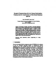
procedure ACO begin Set parameters Initialize pheromone trails repeat construct some candidate solutions Update pheromone trails until a solution is found or maximum number of iterations reached end Fig. 1. Ant Colony Optimization algorithm

– A rule set R is grounded if there exists an enumeration r1 , . . . , rn of R such that ∀i ∈ {1, . . . , n}, ri is applicable in the set Head({r1 , . . . , ri−1 }). – Let Π be a logic program and A an atom set. The set of Generating Rules of Π wrt. A is R(Π, A) = {r ∈ Π|r is applicable in A and not blocked by A}. Computing a stable model of a logic program Π is equivalent to find a particular subset of rules P ⊆ Π as we show in the next result. Lemma 1. Let P ⊆ Π be a subset of a logic program Π. Head(P ) is a stable model of Π iff P is grounded and P = GR(Π, Head(P )). The main goal of our search method is to find a set of rules P satisfying lemma 1. Such a set of rules P is called the Generator of the stable model Head(P ) and all its rules are said to be applied. It is easy to check that all rules in a Generator P are pairwise compatible. Firstly, the previous lemma entails that a rule can not block another rule in the same Generator. Secondly, if r = b ← a, . . . is a rule in P , it means that a ∈ Head(P ) and then any rule like r = c ← . . . , not a, . . . cannot belong to P . This characteristic is similar to the notion developed in [13] about compatibility between default rules.

3 3.1

Ant Colony Optimization for Stable Models Ant Colony Optimization Principles

Ant Colony Optimization (ACO) [5,4] has been inspired by the observation of the collective behavior of ants when they are seeking food. Every ant puts a little bit of pheromone all along its walk and directs itself by choosing its way taking into account the amount of pheromone left by previous ants on each possible path. Since the pheromone evaporates, these probabilistic choices evolve continuously. This collective behavior, based on a kind of shared memory (pheromone on paths), can be used for the resolution of any optimization problem or constraint satisfaction problem which can be encoded as the search of an optimal path in a graph. Following [19] we can resume the general ACO algorithm as in the figure 1.

484

3.2


Problem Representation

We describe here our original design of an Ant Colony Optimization algorithm for stable model search. Definition 3. We associate to a logic program Π the graph G(Π) = (r ∈ Π ∪ {in, out}, A) where each rule becomes a vertex and in and out are two particular vertices added to the rule set. The arc set A is defined by : A = {(in, r), ∀r ∈ Π | body + (r) = ∅} ∪ {(r, r ) ∈ Π 2 | r = r , r and r are compatible} ∪ {(r, out), ∀r ∈ Π} ∪ {(in, out)} \ {(r, r ), (r , r), ∀r, r ∈ Π | r is a forbidden rule } In addition, each arc (i, j) ∈ A is weighted by an artificial pheromone τi,j which is a positive real number. Example 1. The logic program : a ← not f b ← not c c←a Π= d ← a, not b d ← not d e ← d, not f is represented by the following graph (:- stands for ←) :

f ←b

In the sequel, we identify vertices of the graph (different from in and out) and rules of the logic program and we indifferently use P as a path in the graph (ie a sequence of vertices) or as a set of rules. An admissible path is a cycle free path P from in to out in the graph G(Π). It induces a Candidate Generator by implicitly discarding in and out. Thus, the goal of Ant Colony Optimization is to find an admissible path P such that it is a true Generator of a stable model Head(P ). For instance, in example 1, the path P = in, a ← not f, d ← a, not b, c ← a, e ← d, not f, out leads to a true Generator of the stable model Head(P ) = {a, c, d, e}. The definition 3 in which we try to build the graph G(Π) with the smallest arc set possible is justified by the following remarks : – Since we seek a grounded set of rules, all paths have to begin (just after in) by a rule that is applicable in ∅.


485

– Only compatible rules may belong to the same Generator (see end of section 2) so it is useless to put an arc between two rules which are not compatible. – out has to be the last vertex of every path. – The empty set may be a stable model so we need the arc (in, out). – Since no Generator can contain a forbidden rule we isolate every rule of the form x ← . . . , not x, . . .. By this way no path can contain such rules. During the initialization stage, the pheromone on every arc of the graph is initialized to 1 in order to give equal chances to all paths. During the process this pheromone globally evaporates on all arcs and it increases on arcs that are on good paths in order to concentrate a great number of ants on the most promising parts of the graph. 3.3

The Ant’s Travel

In order to reduce the search space to explore, an ant is not allowed to build any admissible path, since some of them can obviously not lead to a solution2 . We limit its choices to the set defined below. Definition 4. Let an ant be on the last vertex v = last(P ) of a partial path P = in, . . . , v that it is currently building; it can only choose the next vertex in the set :   (last(P ), r) is an arc of G(Π)   N ext(P ) = r ∈ Π r is applicable in Head(P )  ∀r ∈ P, r and r are compatible  Furthermore, as it is usual in the design of an Ant System we introduce a local evaluation function η to weight every possible next vertex. The idea is to give the higher values to the vertices which seem to be the better ones to continue the construction of the Candidate Generator. Definition 5. Let P = in, . . . be a path in the graph G(Π) and r ∈ N ext(P ) a possible rule to choose to continue the path.  1/10 if head(r) ∈ Head(P )     1/10 if ∃r ∈ Π | r is forbidden, not blocked     by P and applicable in P ∪ {head(r)}  η(P, r) = k × 10 with k = card({r ∈ Π | r is forbidden,   applicable in P , not blocked by P and     blocked by r})if this set is non empty    1 otherwise The global idea of the heuristic η is based on the fact that a necessary (but not sufficient) condition for a set of atoms to be a true Generator is that it blocks every applicable forbidden rule. This aim is achieved by the four cases of η detailed below. 2

We recall that ants build only cycle free paths but we do not detail how it is done since this is well known.

486


– If the head of a rule is already in the partial Candidate Generator then it seems not really informative to add the same atom again. Furthermore its negative body would still reduce the possible choices of the next rules. – If the head of a rule makes applicable a forbidden rule, we have to avoid to choose it. Indeed, if Π contains a rule like r = b ← a, not b, . . . applying a rule like a ← . . . forces to add in the future a rule which will block r. Otherwise, the resulting set is obviously not a true Generator. – As a supplement of the previous case, we favor a rule if it can block some applicable forbidden rules. – We give a medium value to all of the other rules. This local function combined with the recorded pheromone on the graph leads to the definition of the attractivity of a vertex r for an ant staying on the last vertex of a partial path P = in, . . . . Definition 6. Let G(Π) be a graph for a logic program Π and P = in, . . . , ri a partial path. We define the attractivity of each vertex rj ∈ N ext(P ) by τi,j × η(P, rj ) rk ∈N ext(P ) τi,k × η(P, rk )

A(P, rj ) =

On each vertex ri (the last one of its current path) during its travel from in to out, an ant chooses the next vertex by a random choice between all possible next vertices rj . This choice is biased by the attractivity in such a way that every vertex rj has a probablity to be chosen equal to A(P, rj ). By definition of the set N ext(P ) the only paths that can be explored correspond to rule sets that are grounded. If at any time during the process the set N ext(P ) becomes empty then the ant goes directly to out and the journey is finished. This is the only way for an ant to reach out. Let us remark that the definition of set N ext(P ) ensures that a final path P = in, . . . , out is maximal in the sense that there exists no rule r ∈ Π \ P such that r is applicable in Head(P ) and r is not blocked by Head(P ) except if r is forbidden or if it blocks at least one rule in P . Last, when an ant has chosen its next vertex r, the partial path becomes P = in, . . . , r . If a non-forbidden rule r satisfying   r is applicable in Head(P ) head(r ) ∈ Body − (P )  body − (r ) ⊆ Body − (P ) appears, then the ant goes directly on r because if a Generator S ⊇ P exists then S must contain r . This deterministic inference is applied as long as possible. 3.4

Path Evaluation

Definition 7. Let P be a Candidate Generator for a logic program Π. Its evaluation is defined by : r is applicable in Head(P) eval(P ) = card r ∈Π \P and not blocked by Head(P)


487

By using lemma 1 it is obvious to check that eval(P ) = 0 ⇐⇒ Head(P ) is a stable model of Π. So the goal of the ants is to minimize the value of eval(P ) over the set of possible paths from in to out in G(Π) in order to find a path with a null evaluation. At this point we can informally state that we have a problem of complexity still in class N P , since there is an exponential number of possible paths P , but checking if eval(P ) = 0 can be done in a polynomial time. 3.5

Pheromone Updating

The goal of pheromone updating is to concentrate ants on the paths that minimize the value of eval and this can be done in many various ways. Here we choose an elitist and ranking strategy [2] to update the pheromone trails. So, if the colony contains N ants then we obtain a set S of N ≤ N different paths. If no path has a null evaluation (otherwise a solution is reached) then, we can order S as a sequence of subsets from the better to the worst paths. ∀s ∈ Svi , eval(s) = vi S = Sv1 ∪ . . . ∪ Svn , ∀i > 0, vi < vi+1 If we have fixed to enforce the better paths of S then we determine the least K k value k, 1 ≤ k ≤ n such that i=1 card(Svi ) ≥ K. Given a global reinforcement coefficient ∆, 0 < ∆ < 1, then all paths in Sv1 are reinforced by ∆, those in k−1 Sv2 by ∆2 , . . . , those in Svk−1 by ∆k−1 and, at last, K − i=1 card(Svi ) paths, k randomly chosen in Svk , are reinforced by ∆ . The reinforcement of a path P = in, r1 , . . . , rp , out by a value ∆k does not consist simply in updating the pheromone on arcs (in, r1 ), (r1 , r2 ), . . . , (rp , out). In fact, for a graph G(Π) = (Π ∪ {in, out}, A) all arcs (ri , rj ) ∈ (P × P ) ∩ A are reinforced by ∆k , that is : τi,j + ∆k if (ri , rj ) ∈ Svk and τi,j < 10 τi,j ← τi,j otherwise Therefore, it enables us to record in the pheromone the fact that all the vertices in P seem “to get well together”. Then, an ant of the next colony, standing on a vertex r ∈ P will be more incited to choose any rule r ∈ P even if (r, r ) was not exactly an arc of P . Obviously, this will be possible only if the groundedness condition is respected (this is always checked by the function N ext). Furthermore, we force the pheromone to stay lesser than 10 in order to let a chance to every arc to be chosen by an ant. Finally, the evaporation process acts on every arc (ri , rj ) by : τi,j ← τi,j × 0.99 if τi,j > 0.1 If the pheromone is already lesser than 0.1, we leave it unchanged in order to keep a minimal chance to every arc to be chosen by an ant. On the other side, we force the pheromone trail to stay lesser than 10. It has been shown [19] that this bounding of the pheromone improves the performances of ant systems. To conclude this section, we give in figure 2 the whole general algorithm which includes the different components described above.

488

Pascal Nicolas, Frédéric Saubion, and Igor Stéphan Input : G(Π) the graph representing the logic program M axIt the maximum number of iterations (colonies) N bA the number of ants in the colony N bR the number of paths to be reinforced ∆ the reinforcement coefficient Begin Sol:-false i:-1 Repeat // launch one colony For j:-1 to N bA Do according to the attractivity of every vertex the ant j builds a stochastic admissible path Pj in G If eval(Pj ) = 0 Then Sol:-Pj EndIf EndFor increase pheromone on the N bR better paths let the pheromone evaporate on every arc of the graph i:-i + 1 Until (Sol = f alse) or (i > M axIt) return Sol End Fig. 2. Ant Colony Optimization algorithm

ladder graph : lad_4

board graph : board_4

simplex graph : sim_4

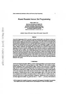
Fig. 3. Graphs for experimental studies

4

Experimental Validation

We have implemented this whole algorithm in a system called ASACO (Answer Set by ACO) using the java language (jdk1.2.2) and we report here some experiments aiming at tuning some parameters monitoring the system : the number of ants in a colony, the number of paths that are reinforced and the rate of this reinforcement. In order to have scalable and understandable examples, we have studied two kinds of problems on graphs : the Hamilton cycle problem and the 3-coloring problem. We used the three kinds of graphs (ladder, board and simplex) presented in figure 3. Both problems have been generated and encoded in a logic program by means of system TheoryBase [3] and we refer to the different problems by the following conventions : ham lad N is an hamiltonian cycle problem on a ladder graph with 2N vertices, ham sim N is an hamiltonian


489

Table 1. Influence of ant colony size ham sim 5 (203 rules) N bA N bR = 5, ∆ = 0.5 N bR = 10, ∆ = 0.9 %suc N bIt %suc N bIt 50 36 21 36 13 100 73 17 70 14 150 96 13 86 9 200 100 11 96 9 300 100 9 100 7 400 100 6 100 4 (M axIt = 1) 5000 20 -

cycle problem on a simplex graph with N vertices on each side and col board N is a 3-coloring problem on a board graph with N 2 vertices. For each test we performed, we ran 30 times our system with exactly the same parameters in order to have a good approximation of its average behavior. In all subsequent tables, results are averages over these 30 runs and we use the following notations : – N bA is the number of ants in a colony. – M axIt is the maximum number of iterations (ie : the maximum number of ant colonies that are launched). – N bR is the percentage of paths or the absolute number of paths (it is mentioned in each case) that are reinforced after each iteration of an ant colony. – ∆ is the basic rate of reinforcement (∆, ∆2 , ∆3 , . . . are used). – %suc is the ratio of the number of runs which find a stable model over the number of all runs. – N bIt is the number of iterations (or colonies) needed to find a solution when the method succeeds. Each problem has at least one stable model and our system stops after having found one or after M axIt iterations. Then, we can use the different rates of success %suc to compare the efficiency of the different choices of values for the parameters. In table 1, we report the influence of the ant colony size. We can see that it is necessary to use a large enough ant colony if we want to be sure to solve the problem in less than M axIt iterations (here M axIt = 30). The best performances are obtained when we reinforce 10 paths with a basic rate ∆ = 0.9 since in this case about 1600 ants (4 colonies of 400 ants) are used to find a stable model in the best case. While at least 2400 ants (6 colonies of 400 ants) are used when only 5 paths are reinforced with a basic rate ∆ = 0.5. So, whatever the updating of pheromone is, a minimal size of the colony is required. For the last line of table 1 we launch 5000 ants at one time and we stop just after one iteration. So, this is a pure stochastic search and the results are very poor : 20 % of success after 5000 tries. So, the general heuristics of Ant Colony Optimization is efficient since, with a good choice of parameters, we obtain 100% of success with less than 2000 tries.

490

Pascal Nicolas, Frédéric Saubion, and Igor Stéphan Table 2. Influence of pheromone reinforcement. ham lad 10 (134 rules) N bA = 100 N bR ∆ = 0.1 ∆ = 0.5 ∆ = 0.9 %suc N bIt %suc N bIt %suc N bIt 0% 50 11 5% 63 12 43 12 50 10 10% 80 9 70 8 76 9 20% 50 9 70 13 86 9 col board 7 (399 rules) N bA = 20 N bR ∆ = 0.1 ∆ = 0.5 ∆ = 0.9 %suc N bIt %suc N bIt %suc N bIt 0% 13 7 5% 13 14 63 19 76 14 10% 20 17 56 17 80 15 ASACO with 600 ants

DLV

SMODELS

14

800 12

600

8

frequency

frequency

10

6 4 2

400

200

[0, 10 0] ]10 0,2 00 ]20 ] 0,3 00 ]30 ] 0,4 00 ]40 ] 0,5 00 ] ]50 0,1 00 0] ]10 00 ,15 ]15 00] 00 ,20 00 ] > 20 00

0

CPU times (sec)

0 [0,10] ]10,20] ]20,30] ]30,40] ]40,50] ]50,60]

>60

number of choice points

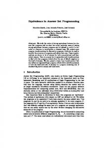
Fig. 4. Comparative results for ham sim 6

In table 2 we report the influence of the pheromone updating on the performance of our system. When N bR = 0%, ∆ has no influence. This explains why there is only one result on these lines. In these cases, the method acts as a pure stochastic search and the percentage of success is again very low. On the other hand, the performances increase with the coefficient of reinforcement and the best results are obtained when at least 10% of the paths are updated. So, once again, this is an argument to demonstrate the efficiency of Ant Colony Optimization. We have made some comparative studies of ASACO versus Smodels [16] and DLV [6]. For these both systems we performed many tests on the same problem by shuffling the input file for each test since we remarked that the performances of these systems may depend on the order of the rules. In figure 4 we detail the distributions of CPU times for Smodels and ASACO for ham sim 6 to illustrate that we are able to obtain interesting results on a problem which is very difficult to solve for one of the best available systems. Even if DLV has very good performances, we can see on the last picture of figure 4 that there exist some configurations of the input file for which the number of explored choice points highly increases.


5

491

Conclusion

In this paper, we have designed an Ant Colony Optimization based algorithm to compute a stable model by trying to determine which rules in the logic program have to be applied together. By lack of time we have not realized a complete set of experiments in order to tune all the parameters that control our system. Nevertheless, the implementation provides performances promising enough to incite us to continue in this way in order to improve the pheromone updating influence and its combination with the local evaluation. Furthermore, we have also developed another implementation in which a step of local search improves some paths built by the ants, and future directions of work are the parallelization of the system.

References 1. Gerhard Brewka and J¨ urgen Dix. Knowledge Representation with Logic Programs. In J. Dix, L. Pereira, and T. Przymusinski, editors, Logic Programming and Knowledge Representation, volume 1471 of LNAI, pages 1–55. Springer Verlag, 1998. 2. B. Bullnheimer, R. Hartl, and C. Strauss. A new rank based version of the ant system — a computational study. Central European Journal of Operations Research, 7(1):25–38, 1999. 3. P. Cholewi´ nski, V. Marek, A. Mikitiuk, and M. Truszczy´ nski. Computing with default logic. Artificial Intelligence, 112:105–146, 1999. 4. D. Corne, M. Dorigo, and F. Glover. New Ideas in Optimization. Mac Graw Hill, 1999. 5. M. Dorigo, E. Bonabeau, and G. Theraulaz. Ant algorithms and stimergy. Future Generation Computer Systems, 16:851–871, 2000. 6. T. Eiter, W. Faber, N. Leone, and G. Pfeifer. Declarative problem solving using the dlv system. In J Minker, editor, Logic Based AI, pages 79–103. Kluwer Academic Publishers, 2000. 7. T. Eiter and G. Gottlob. Complexity results for disjunctive logic programming and application to nonmonotonic logics. In D. Miller, editor, ILP Symposium, pages 266–278. MIT Press, 1993. 8. M. Gelfond and V. Lifschitz. The stable model semantics for logic programming. In Robert A. Kowalski and Kenneth Bowen, editors, Proceedings of the International Conference on Logic Programming, pages 1070–1080. The MIT Press, 1988. 9. M. Gelfond and V. Lifschitz. Classical negation in logic programs and deductive databases. New Generation Computing, 1991. 10. N. Leone, S. Perri, and P. Rullo. Local search techniques for disjunctive logic programs. In E. Lamma and P. Mello, editors, AI*IA’99: Advances in Artificial Intelligence, number 1792 in LNAI, pages 107–118. Springer, 2000. 11. Th. Linke. Graph theoretical characterization and computation of answer sets. In B. Nebel, editor, Proceedings of the IJCAI, pages 641–645. Morgan Kaufmann Publishers, 2001. 12. W. Marek and M. Truszczy´ nski. Autoepistemic logic. Journal of the ACM, 38(3):588–619, 1991. 13. R. Mercer, L. Forget, and V. Risch. Comparing a pair-wise compatibility heuristic and relaxed stratification: Some preliminary results. In S. Benferhat and P. Besnard, editors, Proceedings of ECSQARU, volume 2143 of LNCS, pages 580– 591. Springer Verlag, 2001.

492


14. P. Nicolas, F. Saubion, and I. Stéphan. GADEL : a genetic algorithm to compute default logic extensions. In Proceedings of the European Conference on Artificial Intelligence, pages 484–488, 2000. 15. P. Nicolas, F. Saubion, and I. Stéphan. New generation systems for non-monotonic reasoning. In T. Eiter, M. Truszczynski, and W. Faber, editors, International Conference on Logic Programming and NonMonotonic Reasoning, LNCS, pages 309–321, 2001. 16. I. Niemel¨ a, P. Simons, and T. Syrjanen. Smodels: a system for answer set programming. In Proceedings of the 8th International Workshop on Non-Monotonic Reasoning, Breckenridge, Colorado, USA, 2000. 17. A. Provetti and L. Tari. Answer sets computation by genetic algorithms. In Genetic and Evolutionary Computation Conference, pages 303–308, 2000. 18. R. Reiter. A logic for default reasoning. Artificial Intelligence, 13(1-2):81–132, 1980. 19. T. St¨ utzle and Holger H. Hoos. Max-min ant system. Future Generation Computer systems, 16(8):889–914, 2000.