Dept. of Electronic & Communication Engineering ... target signature and ultimately target classification. .... A simple model, which ignores both the 'tail' of.
Progress In Electromagnetics Research, PIER 27, 1–18, 2000
COMPLEX RESONANT FREQUENCIES FOR THE IDENTIFICATION OF SIMPLE OBJECTS IN FREE SPACE AND LOSSY ENVIRONMENTS Y. Wang Dept. of Computer Science & Electrical Engineering The University of Queensland St Lucia, Brisbane, QLD 4072, Australia N. Shuley Dept. of Electronic & Communication Engineering RMIT University, GPO Box 2476V Melbourne, Victoria, Australia 3001
1. Introduction 2. Theoretical Background 3. Numerical Stimulation 4. Results and Observations References 1. INTRODUCTION The concept of using electromagnetic signals to detect underground objects using ground-penetrating radar (GPR) has been around for decades. Studies concerned with the radiation and scattering problems of buried objects therefore form a significant subset of this concept [1, 2]. Scattering and radiation problems have been traditionally worked in the spectral domain, but in the time domain, the notion of complex natural frequencies arises. The Singularity Expansion Method (SEM) as formalized by Baum [3] is the method by which the transient response of the scattered field is cast in terms of a series of complex exponentials from which these complex resonances can be directly
2
Wang and Shuley
extracted. It is to be noted that SEM does not directly provide the transient response, but rather is an alternative method of looking at the broadband time domain response of boundary value problems and as such is a procedure to be used in conjunction with an analysis procedure. Much attention has been directed toward understanding these complex resonances, as they can form the basis for determination of the target signature and ultimately target classification. The underlying advantage of using such complex resonances for identification is that they are theoretically (in free space) aspect orientation independent and that they form a minimal set of parameters by which the target can be identified thus assisting the classification problem. This means that it is the target shape rather than its orientation that determines the resonances [3] and that the information regarding the target shape is contained in the resonances. It should be noted that this approach is in contrast to methods that image the target directly, e.g., ISAR, and which then apply sophisticated pattern recognition techniques to determine the target. To date, most work has involved target classification in free space as this is of prime consideration to the defence and aerospace communities. For GPR applications, in general, the target resonances will be influenced by the properties of the soil and the airground interface. Whilst Baum’s transformation [2] will provide a first order correction for a target in a lossy homogeneous medium, the whole problem of determining complex resonances needs to be re-examined for the case of the buried target. As a first step towards the buried target problem, we consider a free-space environment with a much simpler target of a thin wire and reconsider the methodology for producing the resonances required for identification algorithms. A number of papers have looked at the transient scattering from thin wires for precisely this purpose [4–9]. The direct method of obtaining the transient response for the target is either by measurement or by solving an integral equation in the time domain or by some other time domain based technique such as FDTD. Prony’s method or similar can then be used to extract the resonances [8, 9]. As an alternative to working in the time domain, the method of moments (MoM) [10], on the other hand, numerically approximates the operator (which depends only on the target characteristics) within which the complex resonances are embedded. One can directly extract the resonances by numerically complex root searching the determinant of the impedance matrix [1, 3, 6], however this is a laborious
Resonant frequencies for the identification of objects
3
and a demanding procedure. In this paper, we choose here instead to obtain the frequency-domain response via MoM and then inverse Fourier transform to the time-domain using the FFT. The resonances are then directly extracted using the generalized pencil-of-function (GPOF) method [11] which is far less noise sensitive and more efficient than Prony’s method. The main advantage of implementing a frequency-domain approach over a time domain approach in the initial step is that the system matrix in the frequency domain is independent of the excitation sources. This results in CPU time savings if the solution for various feeds or incident waves arriving from different directions is required. The procedures in this paper have been chosen so as to be easily applied to the problems of the radiation and scattering of buried bodies in the GPR context by using the frequency domain MoM formulations for layered media [12]. 2. THEORETICAL BACKGROUND The mixed potential electric field integral equation (MPIE) for the current and the charge density on a conducting body S in a known incident field E i is obtained by applying the boundary condition �n × � s ) = 0 on S, where the scattered field E s is expressed in �i + E (E terms of the vector and scalar potentials. The frequency-domain MoM is then applied together with the current continuity equation and using suitable basis functions forms a matrix equation approximation to the MPIE. The unknowns are the induced complex current amplitudes on the perfectly conducting body. For the example of a thin-wire [10] we have: [Z][I] = [V ], (1) where the matrix [Z] is the approximation for the integral equation operator and is only dependent on the geometry and constitutive parameters of the problem. Vector [I] is the unknown current distribution on the wire and vector [V ] is the excitation. The excitation [V ] will normally vary according to different excitations. For the antenna problem, the wire antenna is fed by a time-harmonic source at any point along the wire yielding [V ] = [0, · · · , Vi , · · · , 0],
(2)
where Vi is a unit excitation voltage (delta gap field) applied at ith segment on the thin wire. For the scattering problem, the conducting
4
Wang and Shuley
wire is illuminated from any incidence angle (θ, φ) by an plane wave, in this case the excitation becomes [V ] = [E i (1) · ∆l1 , E i (2) · ∆l2 , · · · , E i (n) · ∆ln ],
(3)
where E i is the incident field of the plane wave and ∆li is the segment length. The impedance matrix [Z] remains unchanged however for both problems. Normally MoM is applied for the time harmonic (single frequency) case. But, if the excitation source is a transient signal, it will contain many frequencies. Its spectrum can be analysed by the FFT. Therefore, spectral weighting is needed before we apply the inverse FFT, to obtain the final time domain response. To extract parameters for target identification proposes [13–16], we choose the complex natural resonance model and express the time-domain signal in SEM representation as: h(t) =
∞ �
Rj eSj t + φ(t)
(4)
j=1
where φ(t) is the entire function, Sj and Rj are the poles and residues, respectively. A simple model, which ignores both the ‘tail’ of the infinite complex exponential series and the contribution of the entire function, is used to represent the late-time response purely in terms of a sum of damped exponentials, each characterized by a complex frequency. The main advantages of this model are that the natural resonances are invariant with target aspect angle and polarization and only a limited number (O(102 )) of identification parameters are needed in a library setup categorizing each scatterer. The GPOF method is then employed to extract the poles and residues from the windowed data of time domain response. Generally, we sample in the late time portion and the number of points to be sampled depends on the numbers of the poles to be extracted. However, we should note that the transient response can only be reproduced starting from the first sampling point. Therefore, if we sample from late time, we can only reproduce the late time signal, which contains the signature of the target. The poles and residues are used to reproduce the time-domain response by: f ((n − 1)∆t) =
N � m=1
cm esm (n−1)∆t ,
(5)
Resonant frequencies for the identification of objects
5
where f ((n−1)∆t) is the transient response at a discrete point of time, Cm are the complex amplitudes or residues, and sm = σm + jωm are the poles, here σm are the damping factors and ωm are the resonant frequencies. It should be mentioned that this is a closed-form expression of the time domain response by the targets natural resonances. Normally, Prony’s or the GPOF methods suffer from spurious poles, however, spurious poles can be distinguished from the real poles by the damping factor and the magnitude of pole coefficient [17]. The complex resonant frequencies can be stored in a library for each object and a neural network technique [13,14] can then be used for the classification of targets. The application of this method to the problems of radiation of buried bodies is conceptually straightforward but difficult. Layered media Green’s functions for both horizontal and vertical electric current sources need to be incorporated. If the object is 3-dimensional, magnetic sources and their corresponding Green’s functions are also required for establishing equivalent surface currents. We have chosen the case of a conducting strip on the interface of a lossy halfspace to illustrate the concept. The MPIE incorporates with rooftop basis functions and Galerkin’s procedure is used [18]. The Greens functions for a lossy halfspace involved in the MPIE are calculated by an easier way which do not directly follow the formulations for a halfspace, that is more difficult to be computed numerically because of two branch cuts [12]. In this case we have chosen to approximate the Green’s functions for the two halfspace problem by selecting a large substrate thickness with a highly lossy dielectric constant, effectively ignoring the ground plane. The vector and scalar Greens functions for a lossy halfspace are calculated by the complex image method using the robust twolevel approximation [19]. The results of this technique are in excellent agreement in the interested frequency range compared with those computed by the exact Sommerfeld integral [18]. It should be noted that the technique will only work when the dielectric constant is sufficiently lossy. After the frequency domain induced current is obtained, the frequency domain scattered field can be calculated by an asymptotic expansion [20]. The determination of the time domain response of the scattered field and complex resonant frequencies is similar to procedures for free space as described above.
6
Wang and Shuley
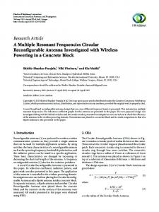
Figure 1. Real and imaginary parts of the spectrum of a Gaussian pulse.
Figure 2. Real and imaginary part of the induced current at the center of a 1m straight wire antenna.
Resonant frequencies for the identification of objects
7
Figure 3. Transient response of the induced current of the 1m straight wire antenna fed by the Gaussian pulse. 3. NUMERICAL SIMULATION To test the approach discussed above, we first consider a 1m dipole antenna with a half length-to-radius ratio of 100. The excitation source is a Gaussian pulse applied across the two center segments of the antenna. The time variation of the Gaussian pulse is taken as exp(−a2 (t − tmax )2 ), where the Gaussian spread parameter a is equal to 5 × 10⁹ s−1 , a time step ∆t of 5.556 × 10⁻¹¹ s is chosen and tmax is 10 × ∆t . The same 1m dipole was first analyzed by Mittra [8] by first using a time domain formulation and then transforming to the frequency domain. This is the reverse process of what is being used here. Although the time domain response was clean, break-up of the spectrum due to numerical instabilities was noticed for the high end of the frequency response. Here the problem is first solved in the spectral domain, using MoM and then transformed to the time domain. The spectrum of the input Gaussian pulse obtained by FFT with 512 sampling points is shown in Fig. 1. It is observed that the Gaussian pulse contains frequencies up to about 4GHz. The induced current at the center of the antenna is then calculated by MoM at each frequency step up to 4GHz and the numerical results are shown in Fig. 2. Since we are using MoM, we expect no numerical instabilities that occurred in
8
Wang and Shuley
the time stepping procedure of [8]. It should be also noted that there is little difference in choosing the primary parameter from which the resonances are extracted. Here we have used the current, however the far field would have been just as suitable and would normally be the measured parameter in a GPR context. Both variables contain similar information about the complex resonances. The frequency response is then inverse Fourier transformed back into the time domain and is shown in Fig. 3. This compares well to the data of [8]. To extract 40 poles and the corresponding residues from the time domain response, 84 samples are actually used which are taken from the first 168 samples (thus including the early time response) at every second time step. This forms the input into the GPOF algorithm, which on output produces the pole pattern of Fig. 4, where the x-axis is the damping factor (Np/ns) and the y-axis is the resonant frequencies (GHz). Only the poles located in the second quadrant of the complex frequency plane are shown, as it can be demonstrated that the poles are simple and only appear in conjugate pairs or lie on the negative real axis [3]. We now consider reconstituting the transient response by using only the poles and residues information extracted from the MPOF algorithm. In the S-plane the poles are actually located in layers [4], with only the first few poles in the first layer (that closest to the imaginary axis) making the more significant contributions to the transient response. First, we observe from Fig. 4 that most of the poles produced by the algorithm are the dominant poles in the first layer with only a few from higher order layers. The reconstitution using all the poles and the first ten pole-pairs is shown in Fig. 3. The original function is well approximated except for minor differences in the early time. This is to be expected as noted previously. A reduced data set consisting of a pole pattern in the s-plane and the corresponding residues is all that is required to reproduce the time domain signature. This fact is of considerable advantage in the identification problem. The second example concerns the scattering of the same straight thin wire illuminated by a parallel polarized plane wave from θ = 60◦ and φ = 0◦ . Fig. 5 shows the frequency domain induced current at the center of the wire and it is noted that this is quite different from the frequency response of Fig. 2. The time-domain current after multiplication by the spectrum of the Gaussian pulse and FFT transformation is shown in Fig. 6. It is noted that the late-time response is now very similar to the case of when the wire was excited as an antenna in Fig. 3,
Resonant frequencies for the identification of objects
9
Figure 4. Poles in the complex frequency plane for the 1m straight wire antenna. but now the early-time response is quite different. This is due to the fact that the early time response includes part local and part global behaviour of the target, whereas the late-time response contains only the global behaviour of the target and is independent of the excitation sources. It is important now that we only sample the late-time response to recover the pole information. Fig. 7 shows the first 20 poles located in the second quadrant extracted from 160 samples of the time domain beginning at 76th sampling point. It can be seen that the first ten poles are almost identical to those of Fig. 4 thus confirming that the complex resonances correspond to the natural frequencies of the object, and as such, are independent of the excitation source. Again only the dominant poles are required to accurately reproduce the time domain signature in late time as demonstrated in Fig. 6. As the third example, Figs. 8 and Fig. 9 show the frequency-domain and corresponding time-domain response of the induced current of an L-shaped wire illuminated by a parallel polarized plane wave from θ = 30◦ and φ = 30◦ . The L-shaped wire is totally 1.0m length with 0.3m and 0.7m arms and the induced current is sampled at 0.2m from the intersection on the 0.7m arm. Fig. 10 shows the pole locations in the complex frequency plane for the L-shaped wire scatterer, which
10
Wang and Shuley
Figure 5. Real and imaginary part of the induced current at the center of the 1m straight wire illuminated by a plane wave.
Figure 6. Time-domain response of the induced current on a 1m straight wire illuminated by the Gaussian pulse.
Resonant frequencies for the identification of objects
11
Figure 7. Poles in the complex frequency plane for the 1m straight wire scatterer. are extracted from 184 samples of the late time. It is observed that the pole pattern of the L-shaped wire is much different from that of the straight wire even though the lengths of both scatterers are the same. We conclude therefore, that pole patterns of various scatterers can be used as a first basis for target identification. The time domain signature recomputed from only the dominant poles functions as a check on the adequacy of the number of terms required in the pole series. In this case we have used all poles to obtain the comparison of Fig. 9, thus demonstrating that higher order poles do not introduce numerical instabilities. Finally, Figs. 11 and 12 show the frequency-domain and the timedomain response of the back scattered field from a conducting strip on the interface of a lossy half space illuminated by a parallel polarized plane wave from θ = 60◦ and φ = 0◦ , where the length and width of the strip is 0.1m and 0.002m, respectively and the complex dielectric constant of the lossy medium is 2.2-j0.22. Here we have approximated the complex dielectric constant by ignoring its frequency dependence. Fig. 13 shows all the poles produced by GPOF method and the identified three true poles in the complex frequency plane for the strip scatterer. For a strip with different length such as 0.15m, The pole pattern is shown in Fig. 14 and it is seen that more resonances happen
12
Wang and Shuley
Figure 8. Real and imaginary part of the induced current at the center of an L-shaped wire illuminated by a plane wave.
Figure 9. Time-domain response of the induced current on the Lshaped wire illuminated by the Gaussian pulse.
Resonant frequencies for the identification of objects
13
Figure 10. Poles in the complex frequency plane for the L-shaped wire scatterer. for a longer strip. It should be noted that the resonant frequencies are different for the cases in Fig. 13 and Fig. 14 though the first three true poles look similar because the axis in the two figures is multiplied by the different length of the targets. 4. RESULTS AND OBSERVATIONS The induced current characteristics for an arbitrarily shaped conducting thin wire antenna and scatterer are analyzed by the frequencydomain method of moments. The corresponding time-domain responses are obtained by the inverse fast Fourier transform after spectrum multiplication. The poles and residues of the transient response are then extracted via the generalized pencil-of-function method. Examples of straight and L-shaped wires in free space are given. It is numerically demonstrated that the poles or complex resonant frequencies are the natural resonances of the conducting thin wire since they are independent of the excitation sources. The pole positions and the corresponding amplitudes can be used to parameterize the transient response and thus may also function as a means for target identification. The application of this method to the problems of radiation and
14
Wang and Shuley
Figure 11. Real and imaginary part of the scattered field from an strip with length 0.1m, width 0.002m and dielectric constant 2.2-j0.22 illuminated by a plane wave.
Figure 12. Time-domain response of the scattered field from the strip with length 0.1m, width 0.002m and dielectric constant 2.2-j0.22 illuminated by the Gaussian pulse
Resonant frequencies for the identification of objects
15
Figure 13. Poles in the complex frequency plane for the strip with length 0.1m, width 0.002m and dielectric constant 2.2-j0.22.
Figure 14. Poles in the complex frequency plane for the strip with length 0.15m, width 0.002m and dielectric constant 2.2-j0.22.
16
Wang and Shuley
scattering of buried bodies is straightforward, requiring only the MoM formulations for layered media. The complex resonances of a strip on a lossy half-space have been analyzed as an example. The subject of how the poles are affected by the lossy medium and depth of the target in the half space is currently under investigation and will be the subject of a subsequent paper. ACKNOWLEDGMENT The authors would like to thank the anonymous reviewer for his/her suggestions and for bringing to our attention references [21, 22]. REFERENCES 1. Vitebiskiy, S., and L. Carin, “Moment-method modeling of shortpulse scattering from and the resonances of a wire buried inside a lossy, dispersive half-space”, IEEE Trans. Antenna Propagat., Vol. AP-43, No. 11, 1303–1312, 1995. 2. Chen, C., and L. Peters, Jr., “Buried unexploded ordnance identification via complex natural resonances”, IEEE Trans. Antenna Propagat., Vol. AP-45, No. 11, 1645–1654, Nov. 1997. 3. Baum, C. E., “The singularity expansion method”, in Transient Electromagnetic Fields, edited by L. B. Felsen, Springer-Verlag, Berlin, 1976. 4. Tesche, F. M., ”On the analysis of scattering and antenna problems using the singularity expansion technique”, IEEE Trans. Antenna Propagat., Vol. AP-21, No. 1, 53–62, Jan. 1973. 5. Richards, M. A., “SEM representation of the early and late time field scattered from wire targets,” IEEE Trans. Antenna Propagat., Vol. AP-42, No. 4, 564–566, April 1994. 6. Richards, M. A., T. H. Shumpert, and L. S. Riggs, “SEM formulation of the fields scattered from arbitrary wire structures,” IEEE Trans. Electromag. Compat., Vol. EMC-35, No. 2, 249–234, May 1993. 7. Richards, M. A., T. H. Shumpert, and L. S. Riggs, ”A modal radar cross section of thin-wire targets via the singularity expansion method,” IEEE Trans. Antenna Propagat., Vol. AP-40, No. 10, 1256–1260, Oct. 1992. 8. Mittra, R., “Integral equation methods for transient scattering,” in Transient Electromagnetic Fields, edited by L. B. Felsen, Springer-Verlag, Berlin, 1976.
Resonant frequencies for the identification of objects
17
9. Van Blaricum, M. L., and R. Mittra, “A technique for extracting the poles and residues of a system directly from its transient response,” IEEE Trans. Antenna Propagat., Vol. AP–23, No. 11, 777-781, Nov. 1975. 10. Harrington, R. F., Field Computation by Moment Methods, MacMillan Company, New York, 1968. 11. Hua, Y., and T. K. Sarkar, “Generalized pencil-of-function method for extracting poles of an EM system from its transient response,” IEEE Trans. Antenna Propagat., Vol. AP-37, No. 2, 229–234, Feb. 1989. 12. Michalski, K. A., and D. Zheng, “Electromagnetic scattering and radiation by surfaces of arbitrary shape in layered media, Part I: Theory, Part II: Implementation and results for contiguous halfspaces,” IEEE Trans. Antennas Propagat., Vol. AP-38, No. 3, 335-352, March 1990. 13. Chen, K. M., E. J. Rothwell, D. P. Nyquist, R. Bebermeyer, Q. Li, C. Y. Tsai, and A. Norman, “Ultra-wideband/short-pulse radar for target identification and detection - laboratory study,” IEEE International Radar Conference, 450–455, New York, USA, 1995. 14. Brooks, J. W., and M. W. Maier, “Application of system identification and neural networks to classification of land mines,” Proceedings of International Conference of The Detection of Abandoned Land Mines, 46–50, London, UK, 1996. 15. Brooks, J. W., and M. W. Maier, “Object classification by system identification and ‘ feature extraction methods applied to estimation of SEM parameters,” IEEE National Radar Conference, 200–205, New York, USA, 1994. 16. Dudley, D. G., “Progress in identification of electromagnetic systems,” IEEE Antennas and Propagation Society Newsletter, 5–11, Aug. 1988. 17. Chen, C. C., L. Peter Jr., and W. D. Burnside, “Ground penetration radar target classification via complex natural resonances,” Proceedings of 1995 IEEE Antennas Propagat. Symposium, Vol. 3, 1586–1589, 1995. 18. Mosig, J. R., “Integral equation technique,” in Numerical Techniques for Microwave and Millimeter-wave Passive Structures, T. Itoh (ed.), Wiley, New York, 1989. 19. Aksun, M. I., “A robust approach for the derivation of closedform Greens functions,” IEEE Trans. Microwave Theory Tech. Vol. 44, No. 5, 651–658, 1996. 20. Uzunoglu, N. K., N. G. Alexopoulos, and J. G. Fikioris, “Radiation properties of microstrip dipoles,” IEEE Trans. Antenna Propagat., Vol. AP-27, 853–858, 1979.
18
Wang and Shuley
21. Baum, C. E. (ed.), Detection and Identification of Visually Obscured Targets, Taylor and Francis, 1998. 22. Hanson, G. W., and C. E. Baum, “Perturbation formula for the natural frequencies of an object in the presence of a layered medium,” Electromagnetics, 333–351, 1998.