Oct 17, 2017 - channels. Rupert H. Leveneâ, Vern I. Paulsenâ, and Ivan G. Todorovâ¡. âSchool of .... tensions of the graph theoretic ones (Theorem IV.10) and.
1
Complexity and capacity bounds for quantum channels Rupert H. Levene∗ , Vern I. Paulsen∗ , and Ivan G. Todorov‡ ∗ School
of Mathematics and Statistics, University College Dublin, Belfield, Dublin 4, Ireland for Quantum Computing and Dept. of Pure Math., University of Waterloo, Waterloo, Ontario, Canada ‡ Mathematical Sciences Research Centre, Queen’s University Belfast, Belfast BT7 1NN, United Kingdom
arXiv:1710.06456v1 [quant-ph] 17 Oct 2017
† Institute
Abstract—We generalise some well-known graph parameters to operator systems by considering their underlying quantum channels. In particular, we introduce the quantum complexity as the dimension of the smallest co-domain Hilbert space a quantum channel requires to realise a given operator system as its non-commutative confusability graph. We describe quantum complexity as a generalised minimum semidefinite rank and, in the case of a graph operator system, as a quantum intersection number. The quantum complexity and a closely related quantum version of orthogonal rank turn out to be upper bounds for the Shannon zero-error capacity of a quantum channel, and we construct examples for which these bounds beat the best previously known general upper bound for the capacity of quantum channels, given by the quantum Lov´asz theta number.
I. I NTRODUCTION In 1956, Shannon [Sha56] initiated zero-error information theory, introducing the concept of the confusability graph GN of a finite input-output information channel N : X → Y . The vertex set of GN is the input alphabet X, and two vertices form an edge in GN if they can result in the same symbol from the output alphabet Y after transmission via N . Shannon showed that the zero-error behaviour of N , and various measures of its capacity, depend only on the graph GN . In particular, if two channels have the same confusability graphs, then they have the same one-shot zero-error capacity and the same Shannon capacity. It is not hard to see that every graph with vertex set X is the confusability graph of some—and in fact many—information channels. Thus, a natural measure of the complexity of a graph G on X is the minimal cardinality of Y over all realisations of G as the confusability graph of a channel N : X → Y . Similarly, Duan, Severini and Winter [DSW13] showed that every quantum channel Φ : Mn → Mk , where Mm denotes the set of complex m × m matrices, has an associated noncommutative confusability graph SΦ , which they defined as a certain operator subsystem of Mn . In the case Φ is a classical channel, SΦ coincides with the graph operator system of GΦ (see [DSW13, equation (3)]). As in Shannon’s case, they proved that many natural measures of the quantum capacity of such a channel depend only on the operator system S. It is again the case that every operator subsystem of Mn arises as the non-commutative confusability graph of potentially many quantum channels.
Thus, we are lead to define the quantum complexity γ(S) of an operator subsystem S of Mn as the least positive integer k for which there exists a quantum channel Φ : Mn → Mk such that S = SΦ . The goal of this paper is to study this and other, closely related, measures of complexity and to derive their relationships with various measures of capacity for classical and quantum channels. We will show, in particular, that the measures of complexity we introduce give upper bounds on the zero-error capacity of a quantum channel. One of the most useful general bounds on the Shannon capacity of a classical channel comes from ϑ, the Lov´asz theta function [Lo79]. While, for classical channels, the complexity based bound is outperformed by the Lov´asz number (see [Lo79, Theorem 11]), we will show that there exist quantum channels for which the quantum complexity bound on capacity we suggest is better than the bounds arising from the noncommutative analogue ϑe of the Lov´asz number introduced in [DSW13]. In fact, we will show that there exist quantum channels Φk for k ∈ N for which the ratio of the quantum e k ) to the quantum complexity γ(Φk ) Lov´asz theta number ϑ(Φ introduced herein is arbitrarily large, while the upper bound γ(Φk ) for the quantum Shannon zero-error capacity Θ(Φk ) is accurate to within a factor of two (see Corollary V.3). We will see that the classical complexity of a graph G is a familiar parameter which coincides with its intersection number (provided G lacks isolated vertices). For operator systems, the measure of quantum complexity we propose has not been previously studied. We will characterise it in several different ways. Since every graph G gives rise to a canonical operator system SG , it can in addition be endowed with a quantum complexity, which can be strictly smaller than its classical counterpart, and can be equivalently characterised as a quantum intersection number of G. The paper is organised as follows. In Section II, we begin by recalling the graph theoretic parameters needed in the sequel and show that our measure of the classical complexity of a graph coincides with its intersection number. In Section III, we turn to the quantum complexity of a graph, and show that it coincides with its minimum semi-definite rank (modulo any isolated vertices). In Section IV, we achieve a parallel development for operator systems, considering simultaneously a closely related notion of subcomplexity that coincides with the quantum chromatic number introduced in [Sta16]. We
2
show that our operator system parameters are genuine extensions of the graph theoretic ones (Theorem IV.10) and explore similarities and differences between their behaviour on commutative and non-commutative graphs. In Section V, we establish the bounds on capacities in terms of complexities (Theorem V.1) and show by example that these bounds can improve dramatically on the Lov´asz ϑ bound. Finally, in Appendix A we establish the partial ordering among various bounds on the quantum Shannon zero-error capacity, from this paper and elsewhere. In the sequel, we employ standard notation from linear algebra: we denote by Mk,n the space of all k by n matrices with complex entries, and set Mn = Mn,n . We let kXk be the operator norm of a matrix X ∈ Mk,n , so that kXk2 is the largest eigenvalue of X ∗ X. We equip Mn with the inner product given by hX, Y i = tr(Y ∗ X), where tr(Z) is the trace of a matrix Z ∈ Mn . We write In (or simply I) for the identity matrix in Mn . The positive cone of Mn (that is, the set of all positive semi-definite n by n matrices) will be denoted by Mn+ ; if S ⊆ Mn , we let S + = S ∩ Mn+ . We write Rk+ for the cone of all vectors in Rk with non-negative entries, and let (ei )ki=1 be the standard basis of Ck . If v, w ∈ Cn , we denote by vw∗ the rank one operator on Cn given by (vw∗ )(z) = hz, wiv, z ∈ Cn . The cardinality of a set S will be denoted by |S|. II. G RAPH PARAMETERS In this section, we recall some graph theoretic parameters and point out their connection with Shannon’s confusability graphs and channel capacities. We start by establishing notation and terminology. Unless otherwise stated, all graphs in this paper will be simple graphs: undirected graphs without loops and at most one edge between any pair of vertices. Let n ∈ N and let G be a graph with vertex set [n] := {1, . . . , n}. For i, j ∈ [n] we write i ' j or i 'G j to denote non-strict adjacency: either i = j, or G contains the edge ij. We denote by Gc the complement of the graph G; by definition, Gc has vertex set [n] and, for distinct i, j ∈ [n], we have i 'Gc j if and only if i 6'Gc j. For graphs H, G with vertex set [n], we write H ⊆ G, and say that H is a subgraph of G, if every edge of H is an edge of G. An independent set in G is a subset of its vertices between which there are no edges of G. Let k ∈ N, and for an n-tuple x = (x1 , . . . , xn ), where each xi ∈ Ck is a non-zero vector, we define G(x) to be the nonorthogonality graph of x, with vertex set [n] and adjacency relation given by i 'G(x) j ⇐⇒ hxj , xi i = 6 0. Let G be a graph with vertex set [n]. Consider the following graph parameters: (a) the independence number α(G) of G, given by α(G) = max{|S| : S is independent in G}; (b) the quantum complexity γ(G) = min{k ∈ N : G(x) = G for some x ∈ (Ck \ {0})n }
and the quantum subcomplexity β(G) = min{k ∈ N : G(x) ⊆ G for some x ∈ (Ck \ {0})n } = min{γ(H) : H is a subgraph of G};
(c) the intersection number int(G) of G, given by int(G) = min{k ∈ N : G(x) = G
for some x ∈ (Rk+ \ {0})n }.
Remark II.1. The graph parameters defined above are well known, and will be generalised to non-commutative graphs in Section IV. (i) The independence number α(G) is standard in graph theory [GR01]. (ii) Writing Gc for the complement of G, we have β(G) = ξ(Gc ) where ξ is the orthogonal rank (see, for example, [SS12]). The parameter γ(G) is the minimum vector rank of G in the terminology of [JMN08], and is equal to msr(G) + | iso(G)| where msr(G) is the classical minimum semidefinite rank of G [FH13], [HPRS15] and iso(G) is the set of isolated vertices of G. (iii) Let intst (G) be the set-theoretic intersection number of G; thus, intst (G) is the smallest positive integer m for which there exist non-empty sets Ri ⊆ [m], i = 1, . . . , n, such that i 'G j if and only if Ri ∩ Rj 6= ∅. (Note that usually in the literature one relaxes the assumption that the sets Ri be nonempty [MM99]; however, it is more convenient for us to work with the definition above.) We claim that int(G) = intst (G). Indeed, first suppose that iso(G) = ∅, and let m = intst (G). Choose Ri ⊆ [m] for i ∈ [n], so that i 'G j ⇐⇒ Ri ∩ Rj 6= ∅. Note that, since P iso(G) = ∅, we have Ri 6= ∅ for every i. Defining xi = r∈Ri er for i ∈ [n], we have that xi ∈ Rk+ , i ∈ [n], and G(x) = G; hence int(G) ≤ k. Conversely, suppose that x = (x1 , . . . , xn ) is a tuple of non-zero vectors in Rk+ such that G(x) = G. Let Ri = {l ∈ [k] : hxi , el i = 6 0}. The non-negativity of the entries of xi , i = 1, . . . , n, implies that i 'G j if and only if Ri ∩Rj 6= ∅; thus, intst (G) ≤ int(G) and so intst (G) = int(G). It is straightforward from the definitions that α(G) ≤ β(G) ≤ γ(G) ≤ int(G)
(1)
for every graph G. We note that these inequalities will be generalised to arbitrary operator systems in Mn in Theorem IV.4 below. We now review some of Shannon’s ideas [Sha56]. Suppose that we have a finite set X, which we view as an alphabet that we wish to send through a noisy channel N in order to obtain symbols from another alphabet, say Y . We let p(y|x) denote the probability that, if we started with the symbol x ∈ X, then after this process, the symbol y ∈ Y is received. We require P that every x ∈ X is transformed into some y ∈ Y , that is, y∈Y p(y|x) = 1, for all x ∈ X. The column-stochastic matrix N = (p(y|x)), indexed by Y ×X, is often referred to as the noise operator of the channel. We will write N : X → Y to indicate the matrix (p(y|x)), and refer to such matrices as (classical) channels. The confusability graph of N is the graph
3
GN with vertex set X for which, given two distinct x, x0 ∈ X, the pair xx0 is an edge if and only if there exists y ∈ Y such that p(y|x)p(y|x0 ) > 0. Equivalently, x 'GN x0 if and only if there exists y ∈ Y such that the symbols x and x0 can be transformed into the same y via N and hence confused. The one-shot zero-error capacity of N , denoted α(N ), is defined to be the cardinality of the largest subset X1 of X such that, whenever an element of X1 is sent via N , no matter which element of Y is received, the receiver can determine with certainly the input element from X1 . It is straightforward that α(N ) = α(GN ).
Fix n ∈ N. Given k ∈ N, we write P(k) for the set of n-tuples P = (P1 , . . . , Pn ) where each Pi is a nonzero projection in Mk . Let Pc (k) denote the subset of P(k) consisting of the elements P = (P1 , . . . , Pn ) with commuting entries: Pi Pj = Pj Pi for all i, j. To any P ∈ P(k) we associate the non-orthogonality graph G(P ) with vertex set [n] and edges defined by the relation
Definition II.2. Let G be a graph with vertex set [n]. The complexity plex(G) of G is the minimal cardinality of a set Y such that G = GN for some channel N : [n] → Y . If N : X → Y is a channel, we set plex(N ) = plex(GN ) and call it this parameter the complexity of N .
qint(G) = min {k ∈ N : G(P ) = G for some P ∈ P(k)} .
Proposition II.3. Let G be a graph with vertex set [n]. Then plex(G) = int(G). In other words, if N : X → Y is a channel then plex(N ) = int(GN ). Proof. Let N : [n] → Y be a channel so that G = GN . For 1 ≤ i ≤ n set Ri = {y ∈ Y : p(y|i) 6= 0}. Then Ri is nonempty for each i and i 'G j ⇐⇒ Ri ∩ Rj 6= ∅. This shows that int(G) is a lower bound for the complexity of G. Conversely, suppose that R1 , . . . , Rn are non-empty subsets of [k] such that i 'G j if and only if Ri ∩ Rj 6= ∅ Set ( 1/|Ri |, y ∈ Ri p(y|i) = ; 0, y∈ / Ri then N = (p(y|i)) is a channel from [n] to [k] with GN = G. This shows that int(G) is an upper bound for the complexity of G. Remark II.4. (i) We will discuss later (Remark IV.11) the natural way to view a classical channel N as a quantum channel; we will see that the quantum complexity of N , studied in Section IV, coincides with γ(GN ). (ii) It is well-known that β(G) ≤ χ(Gc ) for any graph G (here χ(H) denotes the chromatic number of a graph H [GR01]), so it is natural to ask if χ(Gc ) fits into chain of inequalities (1). In fact, it does not: one can check using a computer program that χ(Gc ) ≤ γ(G) for all graphs on 7 or fewer vertices, but this inequality fails in general, for example if x is a KochenSpecker set and G = G(x) (see [HPSWM11, Section 1.2]). (iii) For each π ∈ {α, β, γ, int}, we have that π(G) = 1 if and only if G is a complete graph. Indeed, if G is a complete graph, then π(G) ≤ int(G) = 1, so π(G) = 1; and if G is not a complete graph, then Gc contains at least one edge, so π(G) ≥ α(G) > 1. III. T HE QUANTUM INTERSECTION NUMBER In this section we show that the graph parameter γ, discussed in Section II, has a reformulation in terms of projective colourings of the graph G, which leads to a parameter that we call the quantum intersection number of G. This will allow a key step in the proof of Theorem IV.10, where we show that γ has a natural operator system generalisation.
i 'G(P ) j ⇐⇒ Pi Pj 6= 0. We define the quantum intersection number qint(G) of a graph G with vertex set [n] by letting
The next proposition explains the choice of terminology. Proposition III.1. Let G be a graph with vertex set [n]. Then int(G) = min {k ∈ N : G(P ) = G for some P ∈ Pc (k)} . (2) Proof. Let l be the minimum on the right hand side of (2), and suppose that G(x) = G for some n-tuple x of non-zero vectors in Rk+ . Letting Pi be the orthogonal projection onto the linear span of {er : hxi , er i = 6 0} yields a tuple P = (P1 , . . . , Pn ) ∈ Pc (k) with G(P ) = G; thus, l ≤ int(G). Conversely, suppose that P = (P1 , . . . , Pn ) ∈ Pc (l) is such that G(P ) = G. Simultaneously diagonalising the Pi ’s with respect to a basis {br : r ∈ [l]} and defining Ri = {r ∈ [l] : Pi br 6= 0}, i ∈ [n], we see that i 'G j if and only if Ri ∩ Rj 6= ∅, and it follows that int(G) ≤ l. Pn Let t = (t1 , . . . , tn ) ∈ Nn , and write |t| = i=1 ti . Extending ideas from [HPRS15], let P(k, t) = {(P1 , . . . , Pn ) ∈ P(k) : rank Pi = ti , i ∈ [n]} and define m+ t (G) = min {k ∈ N : G(P ) = G for some P ∈ P(k, t)} . Consider each element A ∈ M|t| as a block matrix A = [Ai,j ]i,j∈[n] where Ai,j ∈ Mti ,tj . We define n + Ft+ (G) = A ∈ M|t| : Ai,j 6= 0 ⇔ i ' j, o and rank(Ai,i ) = ti for each i ∈ [n] and
� Ht+ (G) = A ∈ Ft+ (G) : Ai,i = Iti for each i ∈ [n] .
We write F + (G) = F1+ (G) and H+ (G) = H1+ (G), where 1 = (1, 1, . . . , 1). Note that in [HPRS15], m+t (G) and Ht+ (G) were defined in the special case where t = (r, r, . . . , r) for some r ∈ N. Proposition III.2. Let G be a graph with vertex set [n] and let t ∈ Nn . Then � + m+ t (G) = min rank A : A ∈ Ft (G) � = min rank B : B ∈ Ht+ (G) .
Proof. The proof is an adaptation of [HPRS15, Theorem 3.10]. Suppose first that A ∈ Ft+ (G) and rank A = k. Then there
4
exists a matrix X ∈ Mk,|t| such that A = X ∗ X. Write X = [X1 X2 · · · Xn ], where Xi ∈ Mk,ti , i = 1, . . . , n. We have rank Xi = rank(Xi∗ Xi ) = rank(Aii ) = ti ,
i ∈ [n].
Writing P = (P1 , . . . , Pn ) where Pi ∈ Mk is the orthogonal projection onto the range of Xi , we have P ∈ P(k, t). Additionally, Pi Pj 6= 0 ⇐⇒ Xi∗ Xj 6= 0 ⇐⇒ Ai,j 6= 0 ⇐⇒ i ' j, so G(P ) = G. Hence � + m+ t (G) ≤ min rank A : A ∈ Ft (G) .
Since Ht+ (G) ⊆ Ft+ (G), the inequality � � min rank A : A ∈ Ft+ (G) ≤ min rank B : B ∈ Ht+ (G)
holds trivially. Now suppose that P = (P1 , . . . , Pn ) ∈ P(k, t) with G(P ) = G, and for each i ∈ [n] let Xi ∈ Mk,ti be a matrix whose columns form an orthonormal basis for the range of Pi . Define X = [X1 X2 · · · Xn ] ∈ Mk,|t| and + let B = X ∗ X ∈ M|t| , so that rank B = rank X ≤ k. Note that the ti × tj block Bi,j coincides with Xi∗ Xj . Since i ' j ⇐⇒ Pi Pj 6= 0 ⇐⇒ Xi∗ Xj 6= 0, we have Bij 6= 0 ⇐⇒ i ' j. Moreover, the condition on the columns of Xi implies that Bi,i = Iti for each i. So B ∈ Ht+ (G), hence � min rank B : B ∈ Ht+ (G) ≤ m+ t (G). Theorem III.3. For any graph G, we have qint(G) = γ(G). Proof. Directly from the definitions, we have + qint(G) = minn m+ t (G) ≤ m 1 (G) = γ(G). t∈N
n
Let t ∈ N . We claim that if t1 ≥ 2 and s = (t1 − + 1, t2 , t3 , . . . , tn ), then m+ s (G) ≤ m t (G). By symmetry and in+ n duction, this yields γ(G) = m 1 (G) ≤ m+ t (G) for any t ∈ N , hence qint(G) = γ(G). To establish the claim, suppose that t1 ≥ 2, let k = m+ t (G), and use Proposition III.2 to choose B ∈ Ht+ (G) with rank B = k. We may write B = X ∗ X where X ∈ Mk,|t| . Write X = [X1 X2 · · · Xn ] where Xi ∈ Mk,ti , let Y ∈ Mk,|t|−1 be X with the first column deleted and let Z1 ∈ Mk,t1 −1 be the matrix with every column equal to the first column of X. Let Z = [Z1 0 . . . 0] ∈ Mk,|t|−1 . Let Y1 ∈ Mk,t1 −1 consist of the first (t1 −1) columns of Y . Note that X ∗ Y1 contains X1∗ Y1 as a submatrix, which is equal to It1 with the first column removed. In particular, X ∗ Y1 6= 0. Similarly, the first column of X1∗ Z1 is the first column of It1 , so X ∗ Z1 6= 0. Define a = min{|w| : w 6= 0, w is an entry of X ∗ Y1 } b = max{|w| : w is an entry of X ∗ Z1 }
and let ε ∈ (0, 21 ab−1 ). Define Wε = Y + εZ ∈ Mk,|t|−1 and + A = Aε = Wε∗ Wε ∈ M|t|−1 .
Note that rank A = rank Wε ≤ k. Let us write Wε = [W1 W2 · · · Wn ] and A = [Ai,j ]i,j∈[n] , with block sizes given by s = (t1 − 1, t2 , . . . , tn ). Note that if 2 ≤ i, j ≤ n, then Wi = Xi and Wj = Xj , hence Ai,j = Wi∗ Wj = Xi∗ Xj = Bi,j 6= 0 ⇐⇒ i ' j. Let i ∈ [n]. We have Ai,1 = Xi∗ (Y1 + εZ1 ) = Xi∗ Y1 + εXi∗ Z1 .
(3)
If i 6' 1, then Xi∗ Y1 is a submatrix of Xi∗ X1 = 0, and Xi∗ Z1 is the matrix with every column equal to the first column of Xi∗ X1 = 0. Hence if i 6' 1, then Ai,1 = 0 = A1,i . Now suppose that i ' 1. Since Xi∗ Y1 and Xi∗ Z1 are submatrices of X ∗ Y1 and X ∗ Z1 , respectively, by (3) and our choice of ε, if Xi∗ Y1 has any non-zero entry, then the corresponding entry of Ai,1 is also non-zero. On the other hand, if Xi∗ Y1 = 0, then since i ' 1 yields Xi∗ X1 6= 0, we must have Xi∗ Z1 6= 0, hence Ai,1 6= 0; since A = A∗ , we also have A1,i 6= 0. This shows that for any ε > 0, the matrix A = Aε satisfies Ai,j 6= 0 ⇐⇒ i ' j,
for any i, j ∈ [n].
Since Wε → Y as ε → 0, we see that Aε converges to the matrix B with the first row and column removed; in particular, the top left (t1 − 1) × (t1 − 1) block of Aε converges to It1 −1 . Hence by choosing ε ∈ (0, 21 ab−1 ) sufficiently small, we may ensure that A1,1 has rank t1 − 1, hence A ∈ Fs+ (G). By + Proposition III.2, we have m+ s (G) ≤ rank A ≤ k = m t (G). IV. Q UANTUM CHANNELS AND OPERATOR SYSTEM PARAMETERS
We recall that an operator subsystem of Mn is a subspace S ⊆ Mn such that I ∈ S and X ∈ S =⇒ X ∗ ∈ S. In this paper we will sometimes refer to such a self-adjoint unital subspace S ⊆ Mn simply as an operator system; we refer the reader to [Pau02] for the general theory of operator systems and completely bounded maps. A linear map Φ : Mn → Mk is called a quantum channel if it is completely positive and tracepreserving. By theorems of Choi and Kraus, Φ is a quantum channel if and only if there exists Pm m ∈ N and matrices A1 , . . . , Am ∈ Mk,n , satisfying i=1 A∗i Ai = In , so that Φ(X) =
m X i=1
Ai XA∗i ,
X ∈ Mn .
This realisation of Φ is called a Choi-Kraus representation and the matrices Ai are called its Kraus operators. The ChoiKraus representation is far from unique, but it was shown in [DSW13] that the subspace of Mn spanned by the set {A∗i Aj : 1 ≤ i, j ≤ m} is independent of it. Consequently, [DSW13] set SΦ := span {A∗i Aj : 1 ≤ i, j ≤ m} , Pm where Φ(X) = i=1 Ai XA∗i is any Choi-Kraus representation of Φ. This space, easily seen to be an operator system, is called the non-commutative confusability graph of Φ. Regarding operator subsystems of Mn as non-commutative confusability graphs, we wish to define operator system analogues of the graph parameters considered in Section II. Just as every graph is the confusability graph of some classical
5
channel, [DSW13] showed that the map Φ 7→ SΦ from quantum channels with domain Mn to operator subsystems of Mn , is surjective. We will need the following estimate on the dimension of the target Hilbert space. Proposition IV.1. Let n ∈ N. If S ⊆ Mn is an operator system, then there exists k ∈ N and a quantum channel Φ : Mn �→ Mk such that S = SΦ . In fact, if m ∈ N is such that m 2 ≥ dim S − 1, then we can take k = mn.
Proof. Let d = dim S� and let In , S1 , . . . , Sd−1 be a basis of S. Suppose that m 2 ≥ dim S − 1. Then we can form a hermitian m × m block matrix H = [Hij ]i,j∈[m] ∈ Mm (Mn ) so that Hii = In for i ∈ [m] and {S1 , . . . , Sd−1 } = {Hij : 1 ≤ i < j ≤ m}. 1 For sufficiently small ε > 0, the matrix X = m (Imn + εH) ∗ is positive semi-definite, hence X = C C for some C ∈ Mm (Mn ), and the block entries of X span S. The mn × n block columns of C are then Kraus operators for a quantum channel Φ : Mn → Mmn for which SΦ is spanned by the entries of X, so SΦ = S.
We now define parameters of operator systems which, as we will shortly see, generalise the graph parameters above. Let S ⊆ Mn be an operator system. As usual, we write S ⊥ = {A ∈ Mn : tr(A∗ S) = 0 for all S ∈ S}.
(a) Let S ⊆ Mn be an operator system. Recall [DSW13] that an S-independent set of size m is an m-tuple x = (x1 , . . . , xm ) with each xi a non-zero vector in Cn , so that xp x∗q ∈ S ⊥ whenever p, q ∈ [m] with p 6= q. The independence number α(S) is then defined by letting α(S) = max{m ∈ N : ∃ an S-independent set of size m}. (b) We define the quantum complexity γ(S) by letting γ(S) = min{k ∈ N : SΦ = S
for some quantum channel Φ : Mn → Mk }
and the quantum subcomplexity β(S) by letting β(S) = min{k ∈ N : SΦ ⊆ S
for some quantum channel Φ : Mn → Mk }
= min{γ(T ) : T ⊆ S is an operator subsystem}. (c) A quantum channel Φ which has a set of Kraus operators each of which is of the form AD for some entrywise nonnegative matrix A and an invertible diagonal matrix D will be said to be a non-cancelling. We define int(S) = inf{k ∈ N : SΦ = S for some
non-cancelling quantum channel Φ : Mn → Mk }.
Corollary IV.2. Let S ⊆ Mn be an operator system. Then γ(S) ≤ 2n2 . Proof. Since dim S ≤ n2 , we can take m = 2n in Proposition IV.1.
We will refer to γ(Φ) as the quantum complexity of Φ and β(Φ) as the quantum subcomplexity of Φ. Given a channel Φ, we set π(Φ) = π(SΦ ) for π ∈ {β, γ, int}. Remark IV.3. (i) A set of quantum states can be perfectly distinguished by a measurement system if and only if they are orthogonal. Consequently, [DSW13] defined the one-shot zeroerror capacity α(Φ) of a quantum channel Φ : Mn → Mk to be the maximum cardinality of a set {v1 , ..., vp } ⊆ Cn orthogonal unit vectors, such that tr(Φ(vi vi∗ )Φ(vj vj∗ )) = 0,
i 6= j.
It was shown in [DSW13] (see also [Pau16]) that α(Φ) = α(SΦ ). (ii) Let S be an operator system. The quantum chromatic number χq (S ⊥ ) of the orthogonal complement S ⊥ of S was introduced by D. Stahlke in [Sta16]. It is straightforward that β(S) = χq (S ⊥ ). (iii) For an operator system S ⊆ Mn and π ∈ {β, γ, int}, we have π(S) = 1 ⇐⇒ S = Mn . Indeed, the trace tr : Mn → C is a non-cancelling quantum channel since it has the entrywise non-negative Kraus operators e∗1 , . . . , e∗n (where e∗i is the functional corresponding to the vector ei ), so 1 ≤ π(Mn ) ≤ int(Mn ) = 1 and hence π(Mn ) = 1. Conversely, π(S) = 1 implies that β(S) = 1; the trace is the only scalar-valued quantum channel on Mn , so Mn = Str ⊆ S ⊆ Mn , that is, S = Mn . Note that, in contrast with Remark II.4 (iii), it is not true that Mn is the only operator system S with α(S) = 1; see Proposition IV.12. (iv) We claim that α(CIn ) = β(CIn ) = γ(CIn ) = int(CIn ) = n. Indeed, one sees immediately that α(CIn ) ≥ n by considering the CIn -independent set (e1 , . . . , en ), and since the identity channel Mn → Mn is non-cancelling, we have that int(CIn ) ≤ n, so an appeal to Theorem IV.4 below establishes the claim. (v) Let S ⊆ Mn . Using (iv), we have β(S) = min{γ(T ) : T ⊆ S} ≤ γ(CIn ) = n. On the other hand, γ(S) may exceed n, even for n = 2 (see Proposition IV.12). (vi) There exist operator systems S ⊆ Mn with int(S) = ∞, so the infimum in the definition of int(S) cannot be replaced with a minimum. For example, it is not difficult to see that this is the case for the two-dimensional operator system S� ⊆ M�4 0 X ] where X = 1 1 . spanned by the identity and H = [ X 1 −1 0 Theorem IV.4. Let S ⊆ Mn be an operator system. Then α(S) ≤ β(S) ≤ γ(S) ≤ int(S). Proof. Suppose that Φ : Mn → Mk is a quantum channel with SΦ ⊆ S; let Ai ∈ Mk,n , i = 1, . . . , d, be its Kraus operators. Let (xp )m p=1 be an S-independent set of size m.
6
For each p ∈ [m], let Ep be the projection in Mk onto the span of {Ai xp : i = 1, . . . , d}. Since * d ! + d X X 2 ∗ kAi xp k = Ai Ai xp , xp = 1, i=1
i=1
we have that Ep 6= 0 for each p. On the other hand, since A∗j Ai ∈ S for all i, j = 1, . . . , d and (xp )m p=1 is Sindependent, we have that hAi xp , Aj xq i = hA∗j Ai xp , xq i = 0,
p 6= q, i, j = 1, . . . , d.
Thus, E1 , . . . , Em are pairwise orthogonal projections in Mk ; it follows that m ≤ k and hence α(S) ≤ β(S). The inequalities β(S) ≤ γ(S) ≤ int(S) hold trivially. In the next proposition, we collect some properties of the operator system parameters introduced above. Proposition IV.5. Let S ⊆ Mn and Si ⊆ Mni , i = 1, 2 be operator systems. (i) If π ∈ {α, β, γ} and U ∈ Mn is unitary, then π(U ∗ SU ) = π(S); (ii) If π ∈ {α, β, γ} and P ∈ Mn is a projection of rank r, then, viewing P SP as an operator subsystem of Mr , we have π(P SP ) ≤ π(S); (iii) If π ∈ {β, γ}, n = n1 n2 and S = S1 ⊗ S2 , then max{π(S1 ), π(S2 )} ≤ π(S) ≤ π(S1 )π(S2 ); (iv) If π ∈ {β, γ, int}, n = n1 = n2 and S = span(S1 ∪ S2 ), then π(S) ≤ π(S1 ) + π(S2 ). (v) If π ∈ {β, γ}, then π(S1 ⊕ S2 ) = π(S1 ) + π(S2 ). Proof. The proofs for π = α are easy and are left to the reader. We give the proofs for π = γ; the other proofs follow identical patterns. (i) If {Ap }m p=1 are Kraus operators in Mk,n for which m span{A∗p Aq }m p,q=1 = S, then {Ap U }p=1 are Kraus operators in Mk,n such that ∗ ∗ m span{(Ap U )∗ Aq U }m p,q=1 = U span{Ap Aq }p,q=1 U
= U ∗ SU,
so γ(U ∗ SU ) ≤ γ(S); the reverse inequality follows by symmetry. (ii) If {Ap }m p=1 are Kraus operators in Mk,n for which span{A∗p Aq }m p,q=1 = S, then after identifying the range of P with Cr , we see that {Ap P }m p=1 are Kraus operators in Mk,r with ∗ m span{(Ap P )∗ Aq P }m p=1 = P span{Ap Aq }p,q=1 P = P SP,
so γ(P SP ) ≤ γ(S). (iii) Suppose that {Ap,i : p ∈ [mi ]} ⊆ Mki ,ni is a family of Kraus operators for i = 1, 2, so that Si = span{A∗p,i Aq,i : p, q ∈ [mi ]}, i = 1, 2. Set Bp,r := Ap,1 ⊗ Ar,2 ; then {Bp,r : p ∈ [m1 ], r ∈ [m2 ]} is a family of ∗ Kraus operators in Mk1 k2 ,n with S = span{Bp,r Bq,s : p, q ∈ [m1 ], r, s ∈ [m2 ]}. It follows that γ(S) ≤ γ(S1 )γ(S2 ). If we set P1 = In1 ⊗ Q where Q ∈ Mn2 is a rank one projection, then we have that P1 (S1 ⊗ S2 )P1 = S1 ⊗ C ≡ S1 .
Hence by (ii), π(S1 ) ≤ π(S1 ⊗ S2 ) and the lower bound follows. (iv) Let {Ap,i : p ∈ [mi ]} a family of Kraus � be operators ∗ in Mki ,n with S = span A A : p, q ∈ [m ] , i = 1, 2. i q,i i p,i � � � � Set Bp,1 = A0p,1 n and Bp,2 = A0p,2 , viewedo as elements of Mk1 +k2 ,n . Then √12 Bp,i : i = 1, 2, p ∈ [mi ] Kraus operators with
is a family of
∗ ∗ span{Bp,i Bq,j }p,q,i,j = span{Bp,i Bq,i }p,q,i = S,
so γ(S) ≤ k1 + k2 . Hence, γ(S) ≤ γ(S1 ) + γ(S2 ). (v) If S = S1 ⊕ S2 , then n = n1 + n2 . Suppose that γ(S) = k, so that there exists a family {Cp = [Ap Bp ] : p ∈ [m]} of k × n-Kraus operators, where Ap ∈ Mk,n1 and k,n h A∗BAp ∈A∗M i 2, p q p Bq ∗ with S = span{Cp∗ Cq }m . Since C C = ∈ p q p,q=1 Bp∗ Aq Bp∗ Bq ∗ S1 ⊕ S2 , we have Ap Bq = 0, hence the ranges of Ap and Bq are orthogonal for every p, q. The projections P1 and P2 onto the linear span of the ranges of A1 , . . . , Am and B1 , . . . , Bm are therefore orthogonal, so if k1 = rank P1 and k2 = k − rank P1 ,htheni there is a unitary U : Ck → Ck1 ⊕Ck2 for which h i 0 0 U Ap = A0p for some k1 ×n matrices A0p , and U Bp = Bp0 0 ∗ ∗ for h some k2 × n i matrices Bp . Now Cp Cq = (U Cp ) (U Cq ) = A0p ∗ A0q 0 0 Bp0 ∗ Bq0
, and it follows that γ(Si ) ≤ ki for i = 1, 2. Hence, γ(S1 ) + γ(S2 ) ≤ k1 + k2 = k = γ(S). Combined with (iv), this shows that γ(S1 ⊕ S2 ) = γ(S1 ) + γ(S2 ).
Remark IV.6. (i) Let π ∈ {α, β, γ} and d ∈ N. Then π(Md (S)) = π(S). Indeed, by Proposition IV.5 (ii), we have π(S) ≤ π(Md (S)), and the reverse inequality for π ∈ {β, γ} follows from Proposition IV.5 (iii) and Remark IV.3 (iii). To see the corresponding result for π = α, suppose that {ξp }m p=1 is an independent set for S ⊗Md . Then for X, Y ∈ Md , A ∈ S and p 6= q, we have h(A ⊗ I)(I ⊗ X)ξp , (I ⊗ Y )ξq i = 0
(4)
Let Qp be the projection onto span {(I ⊗ X)ξp : X ∈ Md }; then Qp = Ep ⊗ Id for some non-zero projection Ep on Cn , and (4) implies that Eq SEp = {0} provided p 6= q. If vp is a unit vector with Ep vp = vp , p ∈ [m], we therefore have that {vp }m p=1 is an independent set for S. It follows that α(S) ≥ α(Md (S)) and hence we have equality. (ii) The parameter γ is neither order-preserving nor orderreversing for inclusion. For example, CI2 ⊆ S ⊆ M2 where S is the operator system of Proposition IV.12, and these operator systems have γ-values 2, 3, 1, respectively. We will now show that like its graph-theoretic counterpart, namely, the minimum semidefinite rank, γ(S) is the solution to a rank minimisation problem. Proposition IV.7. For any operator system S ⊆ Mn , we have � γ(S) = min rank B : B = [Bi,j ] ∈ Mm (S)+ with m∈N � m X span{Bi,j : i, j ∈ [m]} = S and Bi,i = In i=1
7
quantum channel. The assertion about non-cancelling channels follows trivially.
and �
β(S) = min rank B : B = [Bi,j ] ∈ Mm (S)+ m∈N
and
m X i=1
�
Bi,i = In .
Moreover, the minima on the right hand sides are achieved for m not exceeding 2n3 . Proof. Suppose that m ∈ N and that B = [Bi,j ]P ∈ Mm (S)+ m m satisfies the relations span{Bi,j }i,j=1 = S and i=1 Bi,i = ∗ In . Then B = A A for some A = [A1 . . . Am ] ∈ M1,m (Mk,n ) where k = rank B. Since Bi,j = A∗i Aj , we see that {A1 , . . . , Am } are Kraus operators for a quantum channel Φ with SΦ = S; thus, γ(S) ≤ k. Conversely, let k = γ(S), m ∈ N and A1 , . . . , Am ∈ Mk,n be Kraus operators for a quantum channel Φ with SΦ = S. Set B := [A∗i Aj ] ∈PMm (S)+ ; we have span{A∗i Aj : m ∗ i, j ∈ [m]} = S, i=1 Ai Ai = In and rank B = rank[A1 . . . Am ] ≤ k. Hence the minimum rank in the first expression is no greater than γ(S). To see that some m ≤ 2n3 attains this minimum, set k = γ(S). Then there exists a quantum channel Φ : Mn → Mk with SΦ = S and, by Corollary IV.2, k ≤ 2n2 . By [Ch75, Remark 6], the channel Φ can be realised using at most nk ≤ 2n3 Kraus operators. Since m is precisely the number of Kraus operators in the preceding argument, we see that the minimum in the expression for γ(S) is attained for some m ≤ 2n3 . The expression for β(S) follows from the fact that β(S) = min{γ(T ) : T ⊆ S}. Since the bound on m for γ, namely 2n3 , is independent of the operator system S ⊆ Mn , this fact shows that here we may also take m ≤ 2n3 . Our next task is to show that the operator system parameters just defined generalise the graph parameters of Section II. Recall that if G is a graph with vertex set [n], we let SG = span{Ei,j : i ' j} be the associated operator subsystem of Mn . Lemma IV.8. Let n, k ∈ N, and let ∆ be the group of diagonal n × n matrices whose diagonal entries are each either 1 or −1. Let x = (x1 , . . . , xn ) be an n-tuple of non-zero vectors in Ck , and let A = [ˆ x1 · · · x ˆn ] be the k × n matrix whose i-th column is the unit vector x ˆi = kxi k−1 xi . Then the map X ∆x : Mn → Mk , ∆x (X) = 2−n ADXDA∗ , D∈∆
is a quantum channel. Moreover, if xi ∈ Rk+ \ {0}, i = 1, . . . , n, then ∆x is non-cancelling. Proof. For D ∈ ∆, let di ∈ {1, −1} be the i-th diagonal entry of D. We have X X 2−n (DA∗ AD)ij = 2−n hˆ xj , x ˆi i di dj = δij , D∈∆
D∈∆
since if i 6= j then the sum reduces to 0 by symmetry, whereas if i = j then every term inPthe sum is 1. Since each x ˆi is a unit vector, we obtain 2−n D∈∆ DA∗ AD = In , so ∆x is a
Proposition IV.9. Let n, k ∈ N, xi be a non-zero vector in Ck , i = 1, . . . , n, and x = (x1 , . . . , xn ). Then SG(x) = S∆x . Proof. Let S = SG(x) and T = S∆x . Set x ˆi = kxi k−1 xi and A = [ˆ x1 · · · x ˆn ], and note that T is spanned by the operators DA∗ AD0 for D = diag(d1 , . . . , dn ) and D0 = diag(d01 , . . . , d0n ) in ∆. For i, j ∈ [n], we have � X � � X � X DA∗ AD0 = D A∗ A D0 D,D 0 ∈∆, di =d0j =1
D 0 ∈∆, d0j =1
D∈∆, di =1
= 4n−1 Ei,i A∗ AEj,j = 4n−1 hˆ xj , x ˆi iEi,j . If Ei,j ∈ S, then i 'G(x) j, so hˆ xj , x ˆi i 6= 0, hence Ei,j ∈ T . Thus S ⊆ T . On the other hand, S ⊥ is spanned by the matrix units Ei,j with i 6'G(x) j. For such i, j and any D, D0 ∈ ∆, we have (DA∗ AD0 )ji = dj hˆ xi , x ˆj id0i = 0, so Ei,j ∈ T ⊥ . Hence S ⊥ ⊆ T ⊥ as required. Theorem IV.10. For any graph G with vertex set [n] and π ∈ {α, β, γ, int}, we have π(SG ) = π(G). Proof. The case π = α is known [DSW13]. We next consider the case π = γ. If k = γ(G), then there exists x = (x1 , . . . , xn ), where xi ∈ Ck \{0}, i = 1, . . . , n, so that G(x) = G, and hence SG(x) = SG . By Proposition IV.9, SG(x) is the operator system of a quantum channel Mn → Mk , hence γ(SG ) ≤ k = γ(G). Now let k = γ(SG ), so that there are Kraus operators A1 , . . . , Am ∈ Mk,n for a quantum channel Φ : Mn → Mk with SΦ = span{A∗q Ap : p, q ∈ [m]} = SG . Since the column operator with entries Pm A1 , . . . , Am is an isometry, for each i ∈ [n] we have p=1 kAp ei k2 = kei k = 1. In particular, Ap ei 6= 0 for at least one p ∈ [m]. Thus, the projection Pi ∈ Mk onto the span of {Ap ei : p ∈ [m]} is non-zero. Consider the tuple P = (P1 , . . . , Pn ) ∈ P(k). Since SΦ = SG , for i, j ∈ [n] we have i 6'G(P ) j ⇐⇒ Pi Pj = 0
∗ ∗ ⇐⇒ hAp ei , Aq ej i = tr(Eij Aq Ap ) = 0,
⇐⇒ Eij ∈
SΦ⊥
=
⊥ SG
for all p, q ∈ [m]
⇐⇒ i 6'G j.
Hence G(P ) = G. Using Theorem III.3, we obtain γ(G) = qint(G) ≤ k = γ(SG ). The case π = β is similar to the case π = γ; alternatively, see [Sta16, Theorem 12]. Let π = int. Set k = int(G); then there exists a tuple x = (x1 , . . . , xn ) ∈ (Rk+ \ {0})n with G(x) = G. By Proposition IV.9, S∆x = SG(x) = SG . By Lemma IV.8, ∆x is a non-cancelling quantum channel; therefore, int(SG ) ≤ k. In particular, int(SG ) < ∞. Now if k = int(SG ), let Φ : Mn → Mk be a non-cancelling quantum channel such that SΦ = SG . Fix Kraus operators A1 D1 , . . . , Am Dm for Φ
8
where each Ap ∈ Mk,n is entrywise non-negative and each Dp is an invertible diagonal n × n matrix. For i ∈ [n], define Ri = {r ∈ [k] : hAp ei , er i = 6 0 for some p ∈ [m]} . Since the column operator 1 D1 , . . . , Am Dm is Pmwith entries A 2 an isometry, we have p=1 kAp Dp ei k = 1, and so Ri is non-empty for all i ∈ [n]. Let x = (x1 , . . . , xn ) where xi = P r∈Ri er . For i, j ∈ [n], we have i 'G j ⇐⇒ Ej,j SG Ei,i 6= {0}
⇐⇒ ∃ p, q ∈ [m] such that hAp Dp ei , Aq Dq ej i = 6 0
⇐⇒ ∃ p, q ∈ [m] such that hAp ei , Aq ej i = 6 0. Now hAp ei , Aq ej i =
X
r∈[k]
hAp ei , er iher , Aq ej i
and every term in the latter sum is non-negative. It follows that i 'G j ⇐⇒ ∃ p, q ∈ [m], r ∈ [k] with hAp ei , er i = 6 0
and hAq ej , er i = 6 0
⇐⇒ Ri ∩ Rj 6= ∅ ⇐⇒ hxj , xi i = 6 0
⇐⇒ i 'G(x) j.
Hence G = G(x), so int(G) ≤ k = int(SG ). Remark IV.11. Let (p(y|x)) be a k × n non-negative columnstochastic matrix defining a classical channel N : [n] → [k] with confusability graph G = GN . The canonical quantum channel Nq : Mn → P Mk associated with N is defined by setting Nq (Ex,x ) = y∈[k] p(y|x)Ey,y and Nq (Ex,x0 ) = 0 if x 6= x0 . We have that SNq = SG [DSW13] (see also [Pau16]). So we see that γ(G) = γ(SG ) is the quantum complexity of the classical channel N when viewed as a quantum channel. Let G � H denote the strong product of the graphs G and H [Sa60], in which (x, y) 'G�H (x0 , y 0 ) if and only if x 'G x0 and y 'H y 0 . Note that SG�H = SG ⊗ SH . If G, H are graphs and n is the number of vertices of G, then (i) α(G) = 1 if and only if G = Kn , i.e., if and only if SG = Mn ; (ii) γ(G) ≤ n; and (iii) γ(G � H) ≤ γ(G)γ(H), but it is unknown whether strict inequality can occur. The following proposition shows that the parameters for general operator systems S ⊆ Mn behave quite differently, with respect to the latter properties, than their graph theoretic counterparts. �� λ a � Proposition IV.12. Let S = b λ : a, b, λ ∈ C . Then α(S) = 1, β(S) = 2, γ(S) = int(S) = 3 and γ(S ⊗ S) < γ(S)2 . h1 0i Proof. The Kraus operators A1 = √12 0 0 and A2 = 01 h0 0i √1 01 yield a non-cancelling quantum channel with op2 10 erator system� S, �so γ(S) ≤ int(S) ≤ 3. Since S ⊥ is 0 spanned by 10 −1 , it contains no rank one operators, and hence α(S) = 1. By Remark IV.3 (v), β(S) ≤ 2 while, by Remark IV.3 (iii), β(S) 6= 1; thus, β(S) = 2.
If γ(S) ≤ 2, then there are Aj = [vj wj ] ∈ M2 for some vj , wj ∈ C2 which are the Kraus operators of a quantum channel with operator system S. We have hvj , vi i = (A∗i Aj )11 = (A∗i Aj )22 = hwj , wi i for each i, j. It follows that there isPa 2 × 2 unitary U with U vj = wj , j = 1, 2. 2 Recall that i=1 A∗i Ai = I2 . This is equivalent to 2 X i=1
and
2 X i=1
2 X
kvi k2 =
hwi , vi i =
i=1
2 X i=1
kwi k2 = 1
hU vi , vi i = 0.
In particular, 0 lies in the numerical range of U . However, the numerical range of a normal matrix is the convex hull of its spectrum, and hence σ(U ) = {α, −α} for some α ∈ T. Thus αU is hermitian, and so U = α2 U ∗ . Now � � hv ,vi i hU vj ,vi i A∗i Aj = hU ∗jvj ,v i i hU vj ,U vi i � 2 = hvj , vi iI + hU ∗ vj , vi i 01 α0 , hence 3 = dim S = dim span{A∗i Aj } ≤ 2, a contradiction. To see that γ(S ⊗ S) < γ(S)2 = 9, consider the isometries Vi ∈ M8,4 given by V1 = [e1 e2 e3 e4 ],
V2 = [e2 e5 e4 e6 ],
V3 = [e3 e4 e7 e8 ],
V4 = [e6 e7 e5 e1 ].
Let W = 21 [V1 V2 V3 V4 ] ∈ M8,16 ; then 0000 0000 1 ∗ W W = 4
00 1000 0000 00 0000 1000 00 0010 0100 00
I4
0 0 0 0
0 0 0 0
1 0 0 0
0 0 0 0
0 0 1 0
0 0 0 0
0 0 0 0
1 0 0 0
0 1 0 0
0 0 0 0
0 0 0 0
0 1 0 0
0 0 0 0
0 0 0 1
0 0 0 0
0 0 0 0
0 0 0 0
0 0 0 0
0 0 1 0
0 0 0 0
1 0 0 0
I4
0 0 1 0
0 0 0 0
0 0 0 0
I4 0 0 0 0
0 0 0 0
0 1 0 0
0 0 0 0
0 0 0 0
1 0 0 0
0 0 0 1
0 0 0 0
0 1 0 0
0 0 0 0
0 0 0 0
0 0 1 0
0 0 0 0
0 0 0 0
I4
Writing Bi,j for the (i, j)-th 4 × 4 block of W ∗ W , we observe that span {Bi,j : i, j ∈ [4]} = S ⊗ S
and
4 X
Bi,i = I4 .
i=1
By Proposition IV.7,
γ(S ⊗ S) ≤ rank W ∗ W = rank W = 8. V. A PPLICATIONS TO CAPACITY Let N : X → Y be a classical information channel with confusability graph G. Its parallel use r times can be expressed as a channel N ×r : X r → Y r , for which r Y r r p((ys )s=1 |(xs )s=1 ) = p(ys |xs ), s=1
for xs ∈ X, ys ∈ Y and s = 1, . . . , r. Note that GN ×r = GN � · · · � GN . | {z } r times
9
The Shannon capacity of the channel N : X → Y (or equivalently of the graph G) is the quantity q p Θ(N ) = Θ(G) = lim r α(N ×r ) = lim r α(G�r N ). r→∞
r→∞
(Some authors prefer to use the logarithm of the quantities defined above.) Similarly, if Φ : Mn → Mk is a quantum channel, letting Φ⊗r : Mn⊗r → Mk⊗r be its r-th power, we find SΦ⊗r = SΦ ⊗ · · · ⊗ SΦ . {z } | r times
The analogue of the Shannon capacity of a quantum channel introduced in [DSW13] is the parameter p Θ(Φ) = lim r α(Φ⊗r ). r→∞
Lov´asz [Lo79] introduced his famous ϑ-parameter of a graph and proved that α(N ) ≤ ϑ(G) and that ϑ is multiplicative for strong graph product; hence, Θ(N ) = Θ(GN ) ≤ ϑ(G), for any classical channel, thus giving a bound on the Shannon capacity of classical channels. He also proved [Lo79, Theorem 11] that ϑ(G) ≤ β(G), so that his ϑ-bound is a better bound on the capacity of classical channels than any of the bounds that we derived from complexity considerations. However, as we will shortly show, for quantum channels, β yields a bound on capacity that can outperform ϑ. We note that a different bound on Θ(G), based on ranks of Hermitian matrices in the operator system SGc , was introduced by Haemers in [Hae81]. It is an interesting open question to formulate general non-commutative analogues of Haemers’ parameter. Lov´asz gave many characterisations of his parameter, but the most useful for our purposes is the expression � ⊥ ϑ(G) = max kI + Kk : I + K ∈ Mn+ , K ∈ SG .
The latter formula motivated [DSW13] to define, for any operator subsystem S of Mn , � ϑ(S) = max kI + Kk : I + K ∈ Mn+ , K ∈ S ⊥ ;
note that ϑ(G) = ϑ(SG ). It was shown in [DSW13] that, for any quantum channel Φ, one has α(Φ) = α(SΦ ) ≤ ϑ(SΦ ). However, ϑ is only supermultiplicative for tensor products of general operator systems. This motivated [DSW13] to e which is multiintroduce a “complete” version, denoted ϑ, plicative for tensor products of operator systems and satisfies e ϑ(S) ≤ ϑ(S). This allowed them to bound the quantum capacity of a quantum channel, since q q � � Θ(Φ) = lim r α SΦ⊗r ≤ lim r ϑ SΦ⊗r r→∞ r→∞ q � ≤ lim r ϑe SΦ⊗r = ϑe (SΦ ) . r→∞
These bounds are often difficult to compute. The quantity q limr→∞ r ϑ(SΦ⊗r ) requires evaluation of a limit, each term of which may be intractable, and the possibly larger bound e Φ ) = supn∈N ϑ(SΦ ⊗ Mn ) requires the evaluation of a ϑ(S supremum, although this parameter has the advantage of possessing a reformulation as a semidefinite program [DSW13]. Theorem V.1. For any quantum channel Φ, we have α(Φ) ≤ Θ (Φ) ≤ β (SΦ ) . Proof. Let Φ be a quantum channel and S = SΦ . The inequality α ≤ Θ is well known, and follows immediately from the supermultiplicative property of α. Since β is submultiplicative for tensor products (Proposition IV.5 (iii)) and α is dominated by β (Theorem IV.4), we have p Θ (Φ) = Θ(S) = lim r α (S ⊗r ) ≤ β (S) . r→∞
In the remainder of the section, we will exhibit operator systems for which β(S) � ϑ(S). For k ∈ N, let Sk = {(ai,j )ki,j=1 ∈ Mk : a1,1 = a2,2 = · · · = ak,k }.
It is easy to show directly that ϑ(Sk ) = k. For any m ∈ N, applying the canonical shuffle which identifies Mk ⊗ Mm with Mm ⊗ Mk , we have � Sk ⊗ Mm = (Ai,j )ki,j=1 ∈ Mk (Mm ) : A1,1 = A2,2 = · · · = Am,m . Thus, for any operator system S ⊆ Mm , we have � Sk ⊗ S = (Ai,j )ki,j=1 ∈ Mk (S) : Theorem V.2. We have
A1,1 = A2,2 = · · · = Am,m .
β(Sk ⊗ Sk2 ) ≤ k 2 < k 3 ≤ ϑ(Sk ⊗ Sk2 ). Proof. Let ω be a primitive k-th root of unity. Let S ∈ Mk2 be given by Sei = ei+1 , i = 1, . . . , k 2 , where addition is modulo k 2 , while D ∈ Mk2 be the diagonal matrix with 2 diagonal (1, ω, ω 2 , . . . , ω k −1 ). Note that, if D0 ∈ Mk is the diagonal matrix with diagonal (1, ω, ω 2 , . . . , ω k−1 ), then D = D0 ⊕ · · · ⊕ D0 . We have that Dj S = ω j SDj for any {z } | k times
j ∈ Z, and hence
Dj S i = ω ij S i Dj ,
i, j ∈ Z.
(5)
Any element A of Mk (Sk ⊗ Sk2 ) has the form A = (Cr,s )k−1 r,s=0 , where Cr,s ∈ Sk ⊗ Sk2 for all r, s = 0, . . . , k − 1. In view of the remarks before the statement of the theorem, we may write Cr,s = (Akr+i,ks+j )k−1 i,j=0 , where Akr+i,ks+j ∈ Sk2 for all r, s, i, j = 0, . . . , k − 1, and Akr+1,ks+1 = Akr+2,ks+2 = · · · = A(r+1)k,(s+1)k , for all r, s = 1, . . . , k. Let ukr+i = S kr+i Dr ,
r, i = 0, . . . , k − 1,
10
and B = (u0 , u1 , u2 , . . . , uk2 −1 ) ∈ Mk2 ,k4 .
Set Br,s = (u∗kr+i uks+j )k−1 i,j=0 ; then the matrix
∗ B ∗ B = (Br,s )k−1 r,s=0 = (ukr+i uks+j )r,s,i,j
is positive and has rank at most k 2 . We will show the following: (i) u∗kr+i uks+j ∈ Sk2 , for all r, s, i, j = 0, 1, . . . , k − 1; (ii) u∗kr+1 uks+1 = u∗kr+2 uks+2 = · · · = u∗kr+k−1 uks+k−1 , for all r, s, i = 0, . . . , k − 1, and Pk (iii) r=1 Br,r = kI, which will imply that β(Sk ⊗ Sk2 ) ≤ k 2 . To show (i), note that
u∗kr+i uks+j = D−r S −kr−i S ks+j Ds = D−r S ks−kr+j−i Ds . If ks − kr + j − i 6= 0, then u∗kr+i uks+j has zero diagonal and thus belongs to Sk2 . Suppose that ks − kr + j − i = 0. Then k|(i − j) and hence i = j. If, in addition, r 6= s then u∗kr+i uks+j has zero diagonal and therefore belongs to Sk2 ; if, on the other hand, r = s, then u∗kr+i uks+j = I and hence again belongs to Sk2 . To show (ii), note that for i = 0, . . . , k − 1, we have
Moreover, these statements hold if throughout we replace ϑ e the quantum Lov´asz theta number. by ϑ,
e it suffices to prove these statments for ϑ. Proof. Since ϑ ≤ ϑ, (i) For the first ratio, consider S = Tβ := Sk ⊗ Sk2 and apply Theorem V.2. For the second ratio, let Tγ be the span of the matrices Br,s ∈ Sk ⊗ Sk2 appearing in the proof of Theorem V.2. Then Tγ ⊆ Sk ⊗ Sk2 is an operator system and the set {Br,s } is one of the terms that appear in the minimum that defines γ(Tγ ). Hence, γ(Tγ ) ≤ rank ((Br,s )) ≤ k 2 < k 3 ≤ ϑ(Sk ⊗ Sk2 ) ≤ ϑ(Tγ ). (ii) For π ∈ {β, γ}, consider Rπ := Tπ ⊕ CIk2 ⊆ Mk3 +k2 . For k > 3, by Proposition IV.5 (v) and Remark IV.3 (iv), we have π(Rπ ) = π(Tπ ) + π(CIk2 ) ≤ k 2 + k 2 = 2k 2 = 2α(CIk2 ) ≤ 2α(Rπ ) ≤ 2Θ(Rπ ).
Since ϑ is order-reversing for inclusion of operator systems and Rπ ⊆ (Sk ⊗ Sk2 ) ⊕ CIk2 ⊆ (Sk ⊕ C) ⊗ Sk2 (the second inclusion holds up to a unitary shuffle equivalence) and it is easy to see that ϑ(S ⊕ T ) ≥ ϑ(S) for any operator systems S and T , we have
u∗kr+i uks+i = D−r S −kr−i S ks+i Ds = D−r S k(s−r) Ds .
ϑ(Rπ ) ≥ ϑ(Sk ⊗ C)ϑ(Sk2 ) ≥ k 3 .
In order to show (iii), suppose that i, j ∈ {0, . . . , k − 1} with i 6= j, and, using (5), note that
A PPENDIX
k−1 X
u∗kr+i ukr+j =
r=0
= =
k−1 X
r=0 k−1 X
D−r S −kr−i S kr+j Dr D−r S j−i Dr
r=0 k−1 X
ω −r(j−i)
r=0
!
S j−i .
Since ω is a primitive root of unity, so is ω −1 . Thus, ω −(j−i) is a k-th root of unity with ω −(j−i) 6= 1. It follows that P Pk−1 k−1 −r(j−i) = 0. Thus, r=0 u∗kr+i ukr+j = 0 whenever r=0 ω i 6= j. On the other hand, k−1 X
u∗kr+i ukr+i
r=0
=
k−1 X
I = kI,
r=0
and (iii) is proved. By [DSW13, Lemma 4],
ϑ(Sk ⊗ Sk2 ) ≥ ϑ(Sk )ϑ(Sk2 ) = k 3 , and the proof is complete. Corollary V.3.
(i) The ratios ϑ(S)/β(S) and ϑ(S)/γ(S)
can be arbitrarily large, as S varies over all noncommutative graphs. (ii) For π ∈ {β, γ}, the ratio ϑ(S)/π(S) can be arbitrarily large, as S varies over all non-commutative graphs with 1 2 π(S) ≤ Θ(S) ≤ π(S).
In this appendix, we briefly summarise the order relationships between various bounds on the quantum Shannon zero-error capacity. These may be succinctly described by the directed graph in Figure 1. The parameters αq , χq and χ are defined in [DSW13], and [Sta16, Definition 11]; the reader should swap S and S ⊥ when translating between our non-commutative graphs and Stahlke’s “trace-free noncommutative graphs”. Let S ⊆ Mn be an operator system. As observed in Remark IV.3 (ii), we have χq (S) = β(S). The first two inequalities in the chain q e αq (S) ≤ ϑ(S) ≤ χq (S ⊥ ) ≤ χ(S ⊥ )
appear in [Sta16], following Corollary 20, and the third inequality is a simple consequence of his Proposition 9. The inequality αq (S) ≤ α(S) is immediate from the definitions (and appears in [DSW13, Proposition 2]), and we have seen in Theorems IV.4 and V.1 that α ≤ Θ ≤ β ≤ γ ≤ int. The inequality Θ ≤ ϑe follows immediately from [DSW13, Proposition 2 and Corollary 10], noting √ that in the notation of that paper, log2 Θ = C0 ≤ C0E ; and ϑe ≤ ϑe is trivial. It only remains to prove the incomparability assertions of Figure 1. These follow from the inequalities already established and the examples below. • Let G = C5 be the 5-cycle, and let S = SG . Lov´ asz has √ shown [Lo79] that ϑ(G) = 5 while, for graph operator e G) = systems, as pointed out in [DSW13], we have ϑ(S ϑ(G). It is not difficult to see that α(SG ) = α(G) = 2 < β(G) = β(SG ).
11
ACKNOWLEDGEMENTS
int(S) χ(S ⊥ ) γ(S)
χq (S ⊥ ) = β(S)
e ϑ(S)
√ e ϑ(S)
Θ(S)
α(S)
αq (S) Fig. 1. A directed graph showing the partial order among various parameters bounding the quantum Shannon zero-error capacity Θ(S) of a noncommutative graph S. The ordering π1 (S) ≤ π2 (S) for every operator system S ⊆ Mn is indicated by placing π1 (S) below π2 (S), joined with a path directed towards π1 (S); the absence of a directed path between a pair of vertices indicates that the corresponding parameters are incomparable.
•
So, in this example, q e ϑ(S) < α(S) and
e ϑ(S) < β(S).
Consider G = C6c , the complement of the 6-cycle, and S = SG . It is easy to see directly that γ(S) = γ(G) > 2, and χ(S ⊥ ) = χ(C6 ) = 2, so in this case, χ(S ⊥ ) < γ(S).
•
•
Let S be the operator system of Proposition IV.12 (i.e., in the notation of Section V, S = S2 ). Note that α(S) = 1. We claim that if T is any operator system with α(T ) = 1, then α(S ⊗T ) = 1. Indeed, S ⊗T may be identified with T A ] for T, A, B ∈ all 2 × 2 block matrices of the form [ B T T , and if x, y are non-zero vectors with xy ∗ ∈ (S ⊗ T )⊥ , then writing x = [ xx12 ] and y = [ yy12 ], we obtain xy ∗ = (xi yj∗ )i,j=1,2 ∈ (S ⊗T )⊥ . By considering the offdiagonal entries and the condition α(T ) = 1, it readily follows that x1 = 0 or y2 = 0, and x2 = 0 or y1 = 0. If x1 = 0, then y1 = 0; hence, xy ∗ = 0 ⊕ x2 y2∗ , so x2 y2∗ ∈ T ⊥ , so x = y = 0, a contradiction. The other case proceeds to a similar contradiction, so α(S ⊗ T ) = 1. Hence, in particular, Θ(S) = 1. On the other hand, e ϑ(S) = 2 by [DSW13, p. 1172]; thus, in this case we have q e Θ(S) < ϑ(S).
Finally, let S = CI2 to obtain an example for which e int(S) < ϑ(S),
since the left hand side is 2 by Remark IV.3 (iv), and, as observed in [DSW13], the right hand side is 4.
The authors are grateful to the Fields Institute and the Institut Henri Poincar´e for financial support to attend the Workshop on Operator Systems in Quantum Information and the Workshop on Operator Algebras and Quantum Information Theory, respectively, greatly facilitating our work on this project. The first named author also wishes to thank Helena ˇ Smigoc and Polona Oblak for stimulating discussion of the minimum semidefinite rank. R EFERENCES [Ch75]
M. D. C HOI, Completely positive linear maps on complex matrices, Lin. Alg. Appl. 10 (1975), 285–290. [DSW13] R. D UAN , S. S EVERINI , A. W INTER, Zero-error communication via quantum channels, non-commutative graphs and a quantum Lov´asz θ function, IEEE Trans. Inf. Theory 59 (2013), 1164–1174. [FH13] S. M. FALLAT, L. H OGBEN, Minimum Rank, Maximum Nullity, and Zero Forcing Number of Graphs, Handbook of Linear Algebra, Chapman and Hall, 2013. [GR01] C. G ODSIL AND G. ROYLE, Algebraic graph theory, SpringerVerlag, 2001. [Hae81] W. H AEMERS, An upper bound for the Shannon capacity of a graph, Colloq. Math. Soc. J´anos Bolyai, 25, North-Holland, Amsterdam-New York, 1981 [HPSWM11] G. H AYNES , C. PARK , A. S CHAEFFER , J. W EBSTER , L. H. M ITCHELL, Orthogonal vector coloring, Elec. J. Combin. 17 (2010), no. 1, Research Paper 55, 18 pp. [HPRS15] L. H OGBEN , K. F. PALMOWSKI , D. E. ROBERSON , S. S EVERINI , Orthogonal representations, projective rank, and fractional minimum positive semidefinite rank: connections and new directions, Elec. J. Linear Algebra 32 (2017), 98–115. [JMN08] Y. J IANG , L. H. M ITCHELL , S. K. NARAYAN, Unitary matrix digraphs and minimum semidefinite rank, Lin. Alg. Appl. 428 (2008), 1685–1695. ´ , On the Shannon capacity of a graph, IEEE Trans. [Lo79] L. L OV ASZ Inf. Theory 25 (1979), no. 1, 1–7. [MM99] T. M C K EE , F. M C M ORRIS, Topics in intersection graph theory, SIAM Monographs on Discrete Mathematics and Applications, 1999. [Pau02] V. I. PAULSEN, Completely bounded maps and operator algebras, Cambridge University Press, 2002. [Pau16] V. I. PAULSEN, Entanglement and non-locality, http://www. math.uwaterloo.ca/∼vpaulsen/EntanglementAndNonlocality LectureNotes 7.pdf, 2016. [Sa60] G. S ABIDUSSI, Graph multiplication, Math. Z. 72 (1960), 446–457. [SS12] G. S CARPA AND S. S EVERINI, Kochen-Specker sets and the rank-1 quantum chromatic number, IEEE Trans. Inf. Theory 58 (2012), no. 4, 2524–2529. [Sha56] C. E. S HANNON, The zero error capacity of a noisy channel, IRE Trans. Inf. Theory 2 (1956), no. 3, 8–19. [Sta16] D. S TAHLKE, Quantum zero-error source-channel coding and non-commutative graph theory, IEEE Trans. Inf. Theory 62 (2016), no. 1, 554–577.