Bounds on the Network Coding Capacity for Wireless Random ... - arXiv

Bounds on the Network Coding Capacity for Wireless Random Networks

arXiv:0710.5340v1 [cs.IT] 29 Oct 2007

Salah A. Aly, Vishal Kapoor, Jie Meng, Andreas Klappenecker Department of Computer Science, Texas A&M University College Station, TX - 77843 {salah, vishal, jmeng, klappi}@cs.tamu.edu

Abstract— Recently, it has been shown that the max flow capacity can be achieved in a multicast network using network coding. In this paper, we propose and analyze a more realistic model for wireless random networks. We prove that the capacity of network coding for this model is concentrated around the expected value of its minimum cut. Furthermore, we establish upper and lower bounds for wireless nodes using Chernoff bound. Our experiments show that our theoretical predictions are well matched by simulation results.

I. I NTRODUCTION Traditionally, the information flow in networks is modeled as a multi-commodity flow problem by treating the underlying network as a flow network. Suppose that one source node in a graph has to transfer some information to one destination node (i.e., a unicast situation). By Menger’s theorem [2], the maximum information that can flow is upper bounded by the value of the minimum cut between the source and the destination; this well-known result from classical graph theory is also known as the Max-flow Min-Cut theorem. One can use max-flow min-cut algorithms to compute the maximum throughput for instance for unicast, multicast, and multi-source multicast communications. Recently, Ahlswede, Cai, Li, and Yeung proposed in the seminal paper [1] a new paradigm, called network coding. Their key observation was that traditional store-and-forward networks cannot always achieve the max-flow value, whereas one can achieve this value using network coding. The idea is based on the simple fact that information can be replicated, mixed together and then transmitted over links to save bandwidth. If this is properly done, then the information can be reliably decoded at the receiver nodes, see e.g. [1], [14]. The basic idea of network coding is that the intermediate network nodes can now process, encode, and transmit information. Since its inception by Ahlswede et al., there has been an upsurge of interest in network coding, see for example [3]– [7], [9], [11] and the references therein. Arguably, most network coding publications model the underlying network as a directed acyclic graph and are typically concerned with solving single source multicast or multi-source multicast using deterministic or randomized encoding and decoding schemes. In this paper, we discuss a new model for wireless random networks. In this model, nodes are placed at random locations.

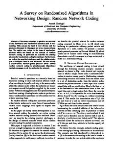
Two nodes u and v are connected with probability 1 if the distance between them is less than or equal to r; the nodes are connected with probability p < 1 if the distance between them is less than or equal to R but greater than r; otherwise u and v are not connected. Thus, the model is a refinement of geometric random graphs that incorporates the potential loss of connectivity towards the end of the transmission range, where interference is more dominant. The main contributions of this paper are: • We introduce the quasi random geometric graph model, a model of wireless network topologies that simulates the connectivity in mobile ad-hoc networks more realistically than the random graph model, but is still easy to analyze. • We derive high-probability bounds for the network coding capacity of quasi random geometric graphs. • We provide simulations results that support our bounds on the network coding capacity. The rest of this paper is organized as follows. In Section II, we give an overview of network coding and the previous work in capacity of network coding. In Section III, we present our new model. We provide our main results in Sections IV and V. II. BACKGROUND AND M ODEL D ESCRIPTION In this section, we give a short summary of network coding, focusing on the calculation of the capacity of a min cut in a weighted random graph. For a more in depth discussion of basic concepts and methods of network coding, we refer the reader to the survey paper [3]. A. Network Coding Fundamentals To illustrate the power of network coding, we provide a simple example, which is often referred to as the Wheatstone bridge, due to its electrical circuits origin. It demonstrates that multicast routing can achieve the maximum possible throughput in a communication network using a coding scheme consisting of linear operations in finite field, whereas traditional store-and-forward routing cannot achieve the same throughput. Consider the example shown in Fig.1(a), where the nodes X and Y respectively want to send two bits b1 and b2 to each other. One way of doing this is to let the bit b1 travel on the path X → A → B → Y at one point of time and to let b2 travel on the path Y → A → B → X on the other. However,

if the network wants to transmit the bits simultaneously, then there is no way to do so, as there are no disjoint paths between X and Y . However, using network coding as shown in Fig. 1(b), one can save bandwidth. In this case, both X and Y transmit the bits b1 and b2 (as shown in the figure) and then A XORs (encodes) them together and the resulting bit b1 ⊕ b2 travels over the paths A → B → Y and A → B → X. Since node X already has of b1 , it can recover (decode) b2 by the operation b1 ⊕ (b1 ⊕ b2 ). Similarly Y can also decode b1 . This example illustrates that the capacity of the minimum cut (equal to 1 in this example) can be easily achieved by network coding, whereas two rounds are needed to achieve the multicast in the uncoded (traditional) routing case, assuming unit capacity edges. Because of such benefits, network coding can be used in wireless ad-hoc networks or sensor networks to help conserve energy and to increase the overall throughput.

Fig. 1.

Graph model (G QRGG ). We derive high-probability bounds for the network coding capacity of such graphs. III. M ODELING R ANDOM W IRELESS N ETWORKS In this section, we present our new model and study the capacity of a minimum cut in a random wireless network. Let r be a real number in the range 0 ≤ r ≤ 1. Recall that a Random Geometric Graph is a graph G RGG = (V, E) with n nodes selected independently and uniformly at random from the unit square [0, 1]2 in which any two nodes u and v in V are connected by an edge (u, v) in E if and only if the Euclidean distance d(u, v) ≤ r. Such a graph is rough approximation of wireless networks. Random geometric graphs have been popular in wireless mobile ad-hoc networks literature, since it is a theoretical model of the network topology that is easy to analyze. However, it does not realistically model the area of transmission, which is, in general, not a disk of radius r. Recently, a more realistic model for connectivity was proposed by Kuhn, Wattenhofer, and Zollinger [10]. In their model, two nodes u and v may or may not be connected when their Euclidean distance d(u, v) is within the range r < d(u, v) ≤ r0 , see Fig. 2. We use random instances of such quasi-disk graphs to model the dynamically changing network topology in wireless random ad-hoc networks.

An example of network coding on a Wheatstone Bridge

B. Network Coding in Ad-hoc Wireless Networks In [13], Ramamoorthy et al. modeled the capacities of the connected edges in a wireless network as a Weighted Random Geometric Graph (G W RGG ) and considered the single source multicast problem. Definition 1 (Single Source Multicast Problem): Let G = (V, E) be a graph with vertex set V and edge set E representing a network. Let S ⊆ V be a set of sources (origins) and T ⊆ V be a set of terminals (destinations). The multicast problem is to distribute the messages from the senders s ∈ S to all terminal nodes t ∈ T , allowing routing along the edges of G. In network coding, the vertices are allowed to encode the incoming bits (or packets) and send encoded versions along the outgoing edges. A single source multicast problem is the special case where one has a single sender, that is, |S| = 1. Ramamoorthy et al. extended the results proved by Karger et al. in [8] and used them to derive bounds for coding capacity for a single source multicast problem in a network comprised of a single source s, an intermediate network consisting of n relay nodes, and l terminal nodes, having independent and identically distributed link capacities ∼ X between any two nodes. They showed that the network coding capacity is concentrated around the value nE[X] in such a network. In this paper, we extend their work to a more general and more realistic model that we call the Quasi Random Geometric

Fig. 2. node

The transmission range and Quasi Disk Graph Representation for a

Definition 2 (Quasi Random Geometric Graph (G QRGG )): Let r and r0 be two real numbers in the range 0 ≤ r < r0 ≤ 1. Let V be a set of n nodes that are selected independently and uniformly at random from the unit square [0, 1]2 . If u and v are two nodes in V , then 1) (u, v) ∈ E if d(u, v) ≤ r; 2) (u, v) ∈ / E if d(u, v) > r0 ; 3) (u, v) ∈ E with probability p if r < d(u, v) ≤ r0 . We call G QRGG = (V, E) a quasi random geometric graph. The difference between quasi random geometric graphs and random geometric graphs is that nodes at distance d within the range r < d ≤ r0 may or may not be connected; this models the connectivity in a more realistic way. Remark 3: Instead of having a fixed probability p for the connectivity of nodes within distance d in the range r < d ≤ r0 , one can use a function p(d) that associates a probability

that depends on the distance to model the attenuation of the signal. Such a change is of course straightforward. We give one example in Section V. In this paper, we consider the problem of single-source multicasts in such quasi random geometric graphs. Our main concern is to provide a lower bound for the capacity of network coding in this situation. Before defining the capacity, we need to further detail our model of connectivity. Definition 4 (Connectivity Graph): Let s be a source node, T a set of terminal nodes, and R a set of relay nodes. We define a connectivity graph G = (V, E) as a graph with vertex set V = {s} ∪ R ∪ T such that G ∈ G QRGG ; in particular, the vertices are located in a unit square. We assume further that the source node only sends messages and terminal nodes only receive messages; in particular, the source and terminal nodes do not relay any messages. Furthermore, we assume that the source and the terminal nodes do not communicate directly; thus, any message is routed through at least one relay node. We assume that the edges in the connectivity graph represent links with unit capacity. Put differently, we assume that the capacity Cij for i, j in V is given by  1 if (i, j) ∈ E, Cij = 0 otherwise. We note that Cij = Cji , since the graph is undirected. Definition 5 (A Cut and its Capacity): Let G = (V, E) be a connectivity graph with source node s, a set T of terminal nodes, and a set R of relay nodes such that V = {s} ∪ R ∪ T . Let t be a terminal node in T . An s-t-cut of size k in the connectivity graph G is a partition of the set of relay nodes R into two sets Vk and V k such that (i) |Vk | = k and |V k | = n − k; (ii) R = Vk ∪ Vk and Vk ∩ Vk = ∅. The edges crossing the cut are given by 1) E ∩ {(s, i)|i ∈ V k }; 2) E ∩ {(j, t)|j ∈ Vk }; 3) E ∩ {(j, i)|j ∈ Vk and i ∈ Vk }. In other words, the source node s and the relay nodes Vk are on one side of the cut, whereas the relay nodes Vk and the terminal node t on the other side of the cut. The total capacity of an s-t-cut of size k is given by X X X X Csi + Cji + Cjt . (1) Ck = i∈Vk

j∈Vk i∈Vk

j∈Vk

IV. B OUNDS AND R ESULTS In this section, we bound the network coding capacity of a connectivity graph, where the connections of the relay nodes form an instance of a quasi random geometric graph. Let G = (V, E) be a connectivity graph such that the vertex set V consists of a source node s, a set of terminal nodes T , and a set of relay nodes R, that is, V = {s} ∪ T ∪ R. Recall that two nodes u and v in G are connected by an edge with probability 1 if d(u, v) ≤ r, with probability p if r < d(u, v) ≤ r0 , and with probability 0 otherwise. Therefore,

the probability p0 that two nodes u and v are connected can be bounded by
1 πr2 + π(r02 − r2 )p ≤ p0 ≤ πr2 + π(r02 − r2 )p. (2) 4 The motivation for the lower bound stems from the fact that one of the nodes might be located in one of the corners of the unit square. The upper bound is a straightforward consequence of our connectivity rules. These elementary observations allow us to bound the expected value of the cut Ck . By equation (1), we have X X X X E[Csi ] + E[Cji ] + E[Cjt ] E[Ck ] = i∈Vk

j∈Vk i∈Vk

j∈Vk

= p0 (n + k(n − k)).

In particular, E[Ck ] = E[Cn−k ] holds for all k in the range 0 ≤ k ≤ n. Furthermore, we have E[C0 ] = E[Cn ] ≤ E[C1 ] = E[Cn−1 ] ≤ · · · ≤ E[Cdn/2e ]. Our goal is to prove that the capacity Ck of an s-t-cut is concentrated around its expected value. A technical difficulty arises because the edges between relay nodes in the graph G are in general not mutually independent. Indeed, if two relay nodes u and v are connected, and u is connected to yet another relay node w, then there is a good chance that v is connected to w. Put differently, we have Pr[(v, w) ∈ E|(u, v) ∈ E, (u, w) ∈ E] > Pr[(v, w) ∈ E], whence the three events (u, v) ∈ E, (u, w) ∈ E, and (v, w) ∈ E are not independent. In Fig. 3, we sketch different geometric situations between two nodes; positioning a node w within the transmission range of u nicely illustrates the intuition behind this fact.

Fig. 3. Consider two relay nodes u and v of G|R . Subfigure (a) illustrates the situation when the two nodes are not connected and far apart. The other subfigures illustrate the following situations: (b) d(u, v) ≤ r, (c) r < d(u, v) ≤ r0 , and (d) 2r < d(u, v) ≤ r + r0 .

However, certain edges in a connectivity graph are independent. Indeed, all edges that are incident with a fixed (common) vertex are independent, since the coordinates of the vertices in the underlying quasi geometric random graph are chosen independently and uniformly at random. Consequently, the random variables in the set {Cij | j ∈ I}, where i is fixed, are independent. We will take advantage of this fact in our

proof of the concentration result. To that end, recall Chernoff’s bound for sums of independent Bernoulli random variables. Lemma 6 (Chernoff bound): Let X1 , . . . , Xm be indepen0 dent Bernoulli random variables such that Pr[X k = 1] = p Pm 0 and Pr[Xk = 0] = 1 − p , and let X = k=1 Xk . For 0 <  < 1, we have 2

Pr[X ≤ (1 − )E[X]] ≤ e−E[X]

/2

.

Proof: See, for instance, [12, p. 66] for a proof of this well-known bound. S Lemma 7: If P r[X + Y ≤ a] ≤ P r[X ≤ a2 ] P r[Y ≤ a2 ]. Proof: This is because if X > a/2 and Y > a/2, definitely X + Y > a. So if X + Y < a, at least one of X and Y must be less than a/2. This lemma is quite simple, but it turns out play a crucial role in the proof of following theorem. Theorem 8: For all cuts of size k, and all , we have
2 (n−k)p0 −ln(k+1) 2 Pr[Ck ≤ (1 − )E[Ck ]] ≤ e− Proof: Let Ck denote the capacity of an s-t-cut ({s} ∪ Vk ; V k ∪ {t}) in the connectivity graph. Here s is the source node, t is a terminal node, and Vk ∪ V k is a partitition of the relay nodes into two disjoint sets Vk and V k that respectively have cardinality k = |Vk | and n − k = |V k |. We can reformulate equation (1) in the form X X X Csi + Cji . (3) Ck = i∈V k

j∈Vk i∈V k ∪{t}

So following lemma 7 and the above formula, if the event Ck ≤ (1 − )E[Ck ]

(4)

happens, then at least one of the following k+1 simpler events must P happen also (i) Pi∈V k Csi ≤ (1 − )E[Ck ]/(k + 1), (ii) i∈V k ∪{t} Cji ≤ (1 − )E[Ck ]/(k + 1), where j ∈ Vk . Since the left hand side of (i) and (ii) are sums of independent Bernoulli random variables, we can use Lemma 6 to bound the probability of these events. Therefore, we obtain the estimate Pr[Ck ≤ (1 − )E[Ck ]] X ≤ Pr[ Csi ≤ (1 − )E[Ck ]/(k + 1)] +

i∈V k X Pr[ j∈Vk

≤ Pr[ +

X

Cji ≤ (1 − )E[Ck ]/(k + 1)]

i∈V k ∪{t}

Csi ≤ (1 − )(k + 1)(n − k)p0 /(k + 1)]

i∈V k X Pr[ j∈Vk

X

X

(Cji ≤ (1 − )(k + 1)

i∈V k ∪{t}

(n − k + 1)p0 /(k + 1))] ≤ exp(−(n − k)p0 2 /2) + k exp(−(n − k + 1)p0 2 /2) ≤ exp(−((n − k)p0 2 /2 − ln(k + 1))).

In the next two theorems, we are going to show that the capacity of a minimum cut is, with high probability, concentrated about the value np0 = E[C0 ]. Intuitively, it is not surprising that the bottleneck is likely going to be the connection from the source to the relay nodes, so the dissemination of the information is likely to be limited. Theorem 9: Let G be a connectivity graph with one source node s, n relay nodes, and a set T of terminal nodes. Then, with probability 1 − O(τ /n2 ), where τ = |T |, the network coding capacity Cs,T of G is bounded from below by s 4 ln n , Cs,T ≥ (1 − )E[C0 ], where  = p0 (n − k) where p0 satisfies (2). Proof: Let Cmin (s, t) denote the capacity of a minimum s-t-cut. Let us assume further that this minimum cut has size k, that is, Cmin (s, t) = Ck . Since E[Ck ] ≥ E[C0 ] holds for all k in the range 0 ≤ k ≤ n, we have Pr[Cmin (s, t) < (1 − )E[C0 ]] ≤ Pr[Ck < (1 − )E[Ck ]] ≤ Pr[|Ck − E[Ck ]| > E[Ck ]]
< 2 exp (−(n − k)p0 2 /2 + ln(k + 1)) , where the last inequality is due to Theorem 8. Substituting the value of  from the hypothesis yields Pr[Cmin < (1 − )E[C0 ]] < 2 exp(−2 ln n) = O(1/n2 ). Consequently, the probability that the network coding capacity Cs,T will be below the value (1 − )E[C0 ] can be bounded by Pr[Cs,T < (1 " − )E[C0 ]] # [ ≤ Pr (Cmin (s, t) < (1 − )E[C0 ]) t∈T X ≤ Pr[Cmin (s, t) < (1 − )E[C0 ]] t∈T

= O(τ /n2 ), as claimed. We complement the above lower bound by a highprobability upper bound on the network coding capacity. Theorem 10: Let G be a connectivity graph with one source node s, n relay nodes, and a set T of terminal nodes. Then, with probability 1 − O(1/n4/3 ), the network coding capacity Cs,T of G is bounded from above by s 4 ln n Cs,T ≤ (1 + )E[C0 ], where  = , E[C0 ] where p0 satisfies (2). Proof: If the network coding capacity Cs,T exceeds the value (1 + )E[C0 ], then the capacity of any s-t-cut, for any t ∈ T , must exceed that value as well; in particular, the cut ({s}; R∪T ) must have capacity exceeding (1+)E[C0 ]. Since

we assume that the source node is not directly connected to any terminal node, we obtain Pr[Cs,T > P(1 + )E[C0 ]] ≤ Pr[ Pr∈R Csr > (1 + )E[C0 ]] ≤ Pr[| r∈R Csr − E[C0 ]| > E[C0 ]] The indicator random variables Csr , with r ∈ R, are mutually independent, as the location of the relay nodes are independently and identically distributed in the unit square. Recall that the Chernoff bound for independent identically distributed indicatorPrandom variables Xi with Pr[Xi = 1] = p0 is given n by Pr[| i=1 Xi − np0 | > t] < 2 exp(−t2 /3np0 ). Applying this Chernoff bound to the indicator random variables Csr yields P Pr[| r∈R Csr − E[C0 ]| > E[C0 ]] 2 2 < 2 exp(− 0 ]))  E[C0 ] /(3E[C 4 ln n E[C0 ]2 = 2 exp − E[C0 ] 3E[C0 ] = O(n−4/3 ),

Fig. 4.

n=200, r=0.1, r0 = 0.2

which proves the claim. Remark 11: Our results easily generalize to more general substrates of unit area (not just unit squares), as long as the assumption holds that the nodes are uniformly distributed over the area. The concentration results are not affected by such a change, but the connectivity probability p0 might be dramatically different. For instance, if the area is a rectangle that is ε high and 1/ε wide, then p0 approaches 0 as ε approaches 0. V. S IMULATIONS AND E XPERIMENTS We conducted simulations for various instances of G QRGG using different parameters. Our simulation results support the high probability bounds on the network coding capacity given in Theorems 9 and 10. In a first experiment, we determined the minimum capacity of an s-t cut for different instances of a connectivity graph in G QRGG with a fixed number of nodes. Fig. 4 shows the results of such an experiment with n = 200 relay nodes. The radio transmission range is chosen such that within a radius of r = 0.1 the connectivity is guaranteed and up to a radius of r0 = 0.2 one might get connected. The plot shows that the capacity of the network is concentrated around the expected value of 13 which is in agreement with Theorem 9 and 10 for the above values of n, r and r0 . Fig. 5 shows the result of a second experiment. This time, the number of relay nodes is once again n = 200, but the transmission range is higher, namely the inner radius equals r = 0.13 and outer radius equals r0 = 0.18. We generated random instances of G QRGG with these parameters and determined the minimum cut. One can easily see that the capacity of the network is likely to be higher, as expected. For larger n, we could observe that the histograms become more concentrated around the expected capacity of a minimum cut, as predicted by our theory.

Fig. 5.

n=200, r=0.13, r0 = 0.18

In a third series of experiments, we simulated the increase of capacity of the minimum cut for different values of r and n. In this case, we also modeled the connectivity probability as a decreasing function of distance, following Remark 3, ! r d(i, j)2 − r2 pconnection , p= 1− r02 − r2 where d(i, j) is the Euclidean distance between any two nodes i and j such that r < |d(i, j)| < r0 , and pconnection is a probability that accounts for the interference noise in communication. As it can be seen from Fig. 6, the value of the capacity grows more rapidly for lower values of r. This is intuitive because in that case not many nodes are connected for small values of n. As we increase n but keep r constant, the capacity of the minimum cut must increase, since more and more nodes are packed in the same area. VI. C ONCLUSION We modeled a quasi wireless random network and showed that the capacity of the minimum cut of network coding is concentrated around the value np0 = E[C0 ]. Unlike prior

Fig. 6.

The capacity of s-t minimum cuts with different values of n and r

works, we obtained high probability bounds for this model. More realistic models (for example, when the probability of connectivity drops exponentially with distance to account for signal attenuation) can be easily incorporated into our framework without changing the theory in a significant way. R EFERENCES [1] R. Ahlswede, N. Cai, S.-Y. R. Li, and R. W. Yeung. Network information flow. IEEE Trans. Info. Theory, 46:1204–1216, 2000. [2] Reinhard Diestel. Graph Theory. Graduate Texts in Mathematics, Volume 173. Springer-Verlag, Heidelberg, third edition edition, July 2005.

[3] C. Fragouli, J. Le Boudec, and J. Widmer. Network coding: An instant primer. ACM SIGCOMM Computer Communication Review, 36(1):63– 68, 2006. [4] T. Ho, R. Koetter, M. Medard, D. Karger, and M. Effros. The benefits of coding over routing in a randomized setting. In Proceedings of the IEEE International Symposium on Information Theory, page 442, Yokohama, Japan, June 2003. [5] T. Ho, M. Medard, R. Koetter, D. R. Karger, M. Effros, J. Shi, and B. Leong. Toward a random operation of networks. submitted to IEEE Trans. Inform. Theory., 2006. [6] T. Ho, M. Medard, J. Shi, M. Effros, and D. R. Karger. On randomized network coding. 41st Annual Allerton Conference on Communication Control and Computing, Oct. 2003. [7] S. Jaggi, P. Sanders, P. A. Chou, M. Effors, S. Egner, and L. M. Tolhuizen. Polynomial time algrithms for multicast network code construction. IEEE Trans. Info. Theory, 51(6), June 2005. [8] D. R. Karger. Random sampling in cut, flow and network design problems. Math. of Oper. Res., 24(2):0383 0413, 1999. [9] R. Koetter and M. Medard. An algebraic approach to network coding. IEEE Trans. on Networking, October 2003. [10] F. Kuhn, R. Wattenhofer, and A. Zollinger. Ad-hoc networks beyond unit disk graphs. 1st ACM Joint Workshop on Foundations of Mobile Computing (DIALM-POMC), San Diego, California, USA, 2003. [11] S.-Y. R. Li, R. W. Yeung, and N. Cai. Linear network coding. IEEE Trans. Inform. Theory, IT-49(2):371381, Feb. 2003. [12] M. Mitzenmacher and E. Upfal. Probability and Computing: Randomized Algorithms and Probabilistic Analysis. Cambridge University Press, 2005. [13] A. Ramamoorthy, J. Shi, and R.D. Wesel. On the capacity of network coding for random networks. IEEE Trans. Info. Theory, 51(8), Aug. 2005. [14] R. W. Yeung. A First Course in Information Theory. Kluwer/Plenum, 2002.