Feb 16, 2018 - Abstract. The classic TQBF problem is to determine who has a winning strategy in a game played on a given CNF formula, where the two ...
Complexity of Unordered CNF Games Md Lutfar Rahman
Thomas Watson
University of Memphis February 16, 2018
Abstract The classic TQBF problem is to determine who has a winning strategy in a game played on a given CNF formula, where the two players alternate turns picking truth values for the variables in a given order, and the winner is determined by whether the CNF gets satisfied. We study variants of this game in which the variables may be played in any order, and each turn consists of picking a remaining variable and a truth value for it. r For the version where the set of variables is partitioned into two halves and each player may only pick variables from his/her half, we prove that the problem is PSPACE-complete for 5-CNFs and in P for 2-CNFs. Previously, it was known to be PSPACE-complete for unbounded-width CNFs (Schaefer, STOC 1976). r For the general unordered version (where each variable can be picked by either player), we also prove that the problem is PSPACE-complete for 5-CNFs and in P for 2-CNFs. Previously, it was known to be PSPACE-complete for 6-CNFs (Ahlroth and Orponen, MFCS 2012) and PSPACE-complete for positive 11-CNFs (Schaefer, STOC 1976).
1
Introduction
Conjunctive normal form formulas (CNFs) are among the most prevalent representations of boolean functions. All sorts of computational problems concerning CNFs—such as satisfying them, minimizing them, learning them, refuting them, fooling them, and playing games on them—play central roles in complexity theory. A CNF is a conjunction of clauses, where each clause is a disjunction of literals; a w-CNF has at most w literals per clause. The width w is often the most important parameter governing the complexity of problems concerning CNFs. The following are three classical games played on a CNF ϕpx1 , . . . , xn q: r In the ordered game, player 1 assigns a bit value for x1 , then player 2 assigns x2 , then player 1
assigns x3 , and so on, and the winner is determined by whether ϕ gets satisfied. Note that the variables must be played in the prescribed order x1 , x2 , x3 , . . .. Deciding who has a winning strategy—better known as TQBF or QSAT—is PSPACE-complete for 3-CNFs [SM73] and in P for 2-CNFs [APT79, Cal08]. Many PSPACE-completeness results have been shown by reducing from the ordered 3-CNF game. r In the unordered game, each player is allowed to pick which remaining variable to play next (as well as which bit value to assign it), and again the winner is determined by whether ϕ gets satisfied. Deciding who has a winning strategy is PSPACE-complete for 6-CNFs [AO12] and
1
for 11-CNFs with only positive literals [Sch76, Sch78]. The unordered game on positive CNFs is also known as the maker–breaker game, and a simplified proof of PSPACE-completeness for unbounded-width positive CNFs appears in [Bys04]. Many PSPACE-completeness results have been proven by reducing from the unordered positive CNF game [FG87, Sla00, Sla02, AS03, Bys04, Hea09, TDU11, vV13, FGM 15, BDK 16]. For the general unordered CNF game, nothing was known for width 6; in particular, the complexity of the unordered 2CNF game was not studied in the literature before. An experimental evaluation of heuristics for the unordered CNF game appears in [ZM04]. r In the partitioned game, the set of variables is partitioned into two halves and each player may only pick variables from his/her half. This is, in a sense, intermediate between ordered and unordered: the ordered game restricts the set of variables available to each player and the order they must be played; the unordered game restricts neither; the partitioned game restricts only the former. Deciding who has a winning strategy was shown to be PSPACEcomplete for unbounded-width CNFs in [Sch76, Sch78], where it was explicitly posed as an open problem to show PSPACE-completeness with any constant bound on the width. This game has been used for PSPACE-completeness reductions [BDG 15], and a variant with a matching between the two players’ variables has also been studied [BI97]. The partitioned 2-CNF game was not studied in the literature before. We prove that the unordered and partitioned games are both PSPACE-complete for 5-CNFs; the former improves the width 6 bound from [AO12], and the latter resolves the 42-year-old open problem from [Sch76, Sch78]. We also prove that the unordered and partitioned games are both in P for 2-CNFs. The complexity for width 3 and 4 remains open. In the following section we give the precise definitions and theorem statements.
1.1
Statement of results
The unordered CNF game is defined as follows. There are two players, denoted T (for “true”) and F (for “false”). The input consists of a CNF ϕ, a set of variables X � tx1 , . . . , xn u containing all the variables that appear in ϕ (and possibly more), and a specification of which player goes first. The players alternate turns, and each turn consists of picking a remaining variable from X and assigning it a value 0 or 1. Once all variables have been assigned, the game ends and T wins if ϕ is satisfied, and F wins if it is not. We let G (for “game”) denote the problem of deciding which player has a winning strategy, given ϕ, X, and who goes first. The partitioned CNF game is similar to the unordered CNF game, except that X is partitioned into two halves XT and XF , and each player may only pick variables from his/her half. If n is even we require |XT | � |XF |, and if n is odd we require |XT | � |XF | 1 if T goes first, and |XF| � |XT| 1 if F goes first. We let G% denote the problem of deciding which player has a winning strategy, given ϕ, the partition X � XT Y XF , and who goes first. % We let Gw and G% w denote the restrictions of G and G , respectively, to instances where ϕ has width w, i.e., each clause has at most w literals. Now, we state our results as the following theorems: Theorem 1. G5 is PSPACE-complete. Theorem 2. G% 5 is PSPACE-complete.
2
Theorem 3. G2 is in P, in fact, in Linear Time. Theorem 4. G% 2 is in P, in fact, in Linear Time. We prove Theorem 1 and Theorem 2 in Section 2 by showing reductions from the PSPACEcomplete games G and G% respectively. For Theorem 3 and Theorem 4 in Section 3 we prove characterizations in terms of the graph representation from the classical 2-SAT algorithm—who has a winning strategy in terms of certain graph properties—and we design linear time algorithms to check these properties.1 In the proofs, it is helpful to distinguish four patterns for ‘who goes first’ and ‘who goes last’, we introduce new subscripts. For a, b P tT, Fu, the subscript a � � � b means player a goes first and player b goes last, a � � � means a goes first, and � � � b means b goes last. These may be combined with the width w subscript. For example, G% T���F (which was denoted G% free pCNFq in [Sch76, Sch78], by the way) corresponds to the partitioned game where T goes first and F goes last (so n � |X | must be even), and G5,���T corresponds to the unordered game with width 5 where T goes last (so either n is even and F goes first, or n is odd and T goes first).
2
5-CNF
We prove Theorem 1 in Section 2.1 and Theorem 2 in Section 2.2.
2.1
G5
In this section we prove Theorem 1. It is trivial to argue that G5 P PSPACE. We prove PSPACEhardness by showing a reduction GT���F ¤ G5,T���F in Section 2.1.2. GT���F is already known to be PSPACE-complete [Sch76, Sch78, Bys04, AO12]. We will talk about the other three patterns GF���F , GT���T , GF���T in Section 2.1.3. Before the formal proof we develop the intuition in Section 2.1.1. 2.1.1
Intuition
In NP-completeness, recall the following simple reduction from SAT with unbounded width to 3SAT. Suppose a SAT instance is given by ϕ over set of variables X. If p`1 _ `2 _ `3 _ � � � _ `k q is a clause in ϕ with width k ¡ 3, then the reduction introduces fresh variables z1 , z2 , . . . , zk�1 and generates a chain of clauses in ϕ1 as follows:
p`1 _ z1q ^ pz1 _ `2 _ z2q ^ � � � ^ pzi�1 _ `i _ ziq ^ � � � ^ pzk�2 _ `k�1 _ zk�1q ^ pzk�1 _ `k q Each clause of ϕ gets a separate set of fresh variables for its chain, and we let Z � tz1 , z2 , . . .u be the set of all fresh variables for all chains. The reduction claims that ϕ is satisfiable if and only if ϕ1 is satisfiable. We are going to have a stronger property in Claim 1. Claim 1. For every assignment x to X: ϕpxq is satisfied iff there exists an assignment z to Z such that ϕ1 px, z q is satisfied. 1 We remark that it is not automatic that two-player games on 2-CNFs are solvable in polynomial time; e.g., the game played on a 2-CNF with only negative literals in which players alternate turns assigning variables of their choice to 0 and where the loser is the first to falsify the 2-CNF, as well as the partitioned variant of this game, are PSPACE-complete [Sch76, Sch78].
3
Proof. Suppose x satisfies ϕ. If x satisfies p`1 _ `2 _ `3 _ � � � _ `k q in ϕ by `i � 1, then in the corresponding chain of clauses in ϕ1 , the clause having `i also gets satisfied by `i � 1 and the rest of the clauses in that chain can get satisfied by assigning all z’s on the left side of `i as 1 and right side of `i as 0. Now suppose x does not satisfy ϕ. Then at least one of the clauses of ϕ has all literals assigned as 0. The corresponding chain of clauses in ϕ1 essentially becomes:
pz1q ^ pz1 _ z2q ^ � � � ^ pzi�1 _ ziq ^ � � � ^ pzk�2 _ zk�1q ^ pzk�1q In order to satisfy the above chain, z1 � 1 and zk�1 � 0. It also introduces the following chain of implications: z1 ñ z2 ñ z3 ñ � � � ñ zk�1 . Following the chain we get (z1 ñ zk�1 ) = (1 ñ 0). Therefore, we conclude that ϕ1 px, z q cannot be satisfied for any assignment z. Now this reduction does not show GT���F ¤ G3,T���F since the games on ϕ and ϕ1 are not equivalent. We show a simple example to make our point. Consider the following GT���F game over variables tx0 , x1 , . . . , xk u. ϕ � x0 ^ px1 _ x2 _ x3 _ � � � _ xk q, where k
¡1
In the above GT���F game, T has a winning strategy: On the first move T plays x0 � 1. Then whatever F plays, T plays one of the k � 1 many unassigned xi from tx1 , x2 , . . . , xk u as 1. T wins. But if we introduce fresh variables tz1 , z2 , z3 , . . .u as in the NP-completeness reduction then we get a game over variables tx0 , x1 , x2 , . . . , xk u Y tz1 , . . . , zk�1 u: ϕ1
� x0 ^ px1 _ z1q ^ � � � ^ pzi�1 _ xi _ ziq ^ � � � ^ pzk�1 _ xk q
In the above G3,T���F game, F has a winning strategy: On the first move T must play x0 � 1, otherwise F wins by x0 � 0. Then F plays x1 � 0 and T must reply by z1 � 1, otherwise F wins by z1 � 0. Then F plays x2 � 0 and T must reply by z2 � 1, otherwise F wins by z2 � 0. The strategy goes on like this until the last clause and F wins by xk � 0. The G3,T���F game is disadvantageous for T compared to the GT���F game. The disadvantage arises from F having the beginning move in a fresh chain of clauses. Now the intuition is to design a game version of the NP-completeness reduction by fixing the imbalance. We design ψ in such a way that the games on ϕ and ψ stay equivalent. In order to counter the unfairness for T due to fresh variables tz1 , z2 , z3 , . . .u, we replace zi by a pair of variables (ai , bi ) which gives T more opportunities to satisfy the clauses. The construction of a chain of clauses in ψ from a clause p`1 _ `2 _ `3 _ � � � _ `k q in ϕ goes as follows:
p`1 _ a1 _ b1q ^ � � � ^ pai�1 _ bi�1 _ `i _ ai _ biq ^ � � � ^ pak�1 _ bk�1 _ `k q We just constructed a 5-CNF ψ. Let us consider the G5,T���F game on ψ. In an optimal gameplay, no player should play a’s or b’s before playing x’s. Intuitively, this is because, if F plays any ai or bi , then T can reply by making ai � bi and both clauses involving ai and bi will be satisfied, which benefits T. If T plays any ai or bi , F can reply by making ai � bi , which satisfies one clause involving ai and bi but the other clause gets two 0 literals. Since only one of the two clauses gets satisfied by ai , bi , T would like to wait for more information before deciding which one to satisfy with ai , bi : it depends on whether they are on the right side or left side of a satisfied `i in a chain, which in turn depends on the assignment x.
4
So, an optimal gameplay consists of two phases. In the first phase, players should play only x’s. Whoever deviates from this optimal strategy does not have the upper hand. The second phase begins when all the x’s have been played and someone must start playing a’s and b’s. Since the number of fresh variables is even (2|Z |) and F plays last, T must be the one to start the second phase, which is essential since if F started the second phase then T could satisfy all the clauses regardless of what happened in the first phase. This observation also allows us to show PSPACE-completeness of G5,F���F , discussed in Section 2.1.3. In the second phase, after T plays any ai or bi , it is optimal for F to reply by making ai � bi . Assuming this optimal gameplay by F, we can consider a pair (ai ,bi ) as a single variable zi which can be assigned only by T. Effectively, the second phase just consists of T choosing an assignment z to ϕ1 from the NP-completeness reduction. Thus ψ px, a, bq is satisfied iff ϕ1 px, z q is satisfied, which by Claim 1 is possible iff ϕpxq is satisfied, where x is the assignment from the first phase. 2.1.2
Formal Proof
We show GT���F ¤ G5,T���F . Suppose an instance of GT���F is given by pϕ, X q where ϕ is a CNF with unbounded width over set of variables X. We show how to construct an instance pψ, Y q for G5,T���F where ψ is a 5-CNF over set of variables Y . Suppose p`1 _ `2 _ `3 _ � � � _ `k q is a clause in ϕ. If k ¤ 3, the same clause remains in ψ. If k ¡ 3, we show how to construct a chain of clauses in ψ. We introduce two sets of fresh variables ta1 , a2 , a3 , . . . , ak�1 u and tb1 , b2 , b3 , . . . , bk�1 u as follows:
p`1 _ a1 _ b1q ^ � � � ^ pai�1 _ bi�1 _ `i _ ai _ biq ^ � � � ^ pak�1 _ bk�1 _ `k q Each clause of ϕ gets separate sets of fresh variables for its chain, and we let A � ta1 , a2 , a3 , . . .u and B � tb1 , b2 , b3 , . . .u be the sets of all fresh variables for all chains. Finally we get a 5-CNF ψ over set of variables Y � X Y A Y B. We claim that T has a winning strategy in pϕ, X q iff T has a winning strategy in pψ, Y q. Suppose T has a winning strategy in pϕ, X q. We describe T’s winning strategy in pψ, Y q as Algorithm 1. To see that the strategy works, note that the winning strategy in pϕ, X q ensures that ϕpxq is satisfied by the assignment x to X in the first phase, so according to Claim 1, there is an assignment z to Z such that ϕ1 px, z q is satisfied. T can ensure that for each i, either ai � zi or bi � zi (since ai � zi or bi � zi due to line 8, or ai � bi due to line 4 or line 7) and thus ψ px, a, bq gets satisfied, since ϕ1 px, z q is satisfied and each clause of ψ is identical to a clause from ϕ1 but with each zi replaced with ai _ bi and z i replaced with ai _ bi . Suppose F has a winning strategy in pϕ, X q. We describe F’s winning strategy in pψ, Y q as Algorithm 2. To see that the strategy works, note that the winning strategy in pϕ, X q ensures that ϕpxq is unsatisfied by the assignment x to X, so according to Claim 1, for all assignments z to Z, ϕ1 px, z q is unsatisfied. F can ensure that for each i, ai � bi ; let us call this common value zi . Thus ψ px, a, bq is unsatisfied, since ϕ1 px, z q is unsatisfied and ψ px, a, bq � ϕ1 px, z q. 2.1.3
GF���F , GT���T , GF���T
Corollary 1. G5,F���F is PSPACE-complete. Proof. The reduction is GT���F ¤ GF���F ¤ G5,F���F . First we show GT���F ¤ GF���F . Suppose ϕ � c1 ^ c2 ^ c3 ^ � � � ^ cm over set of variables X is an instance of GT���F . We introduce a fresh variable z and construct ψ � pc1 _ z q ^ pc2 _ z q ^ pc3 _ z q ^ � � � ^ pcm _ z q over set of variables 5
Algorithm 1: T’s winning strategy in pψ, Y q when T has a winning strategy in pϕ, X q 1 2 3
while there is a remaining X-variable do if (first move) or (F played an X-variable in the previous move) then play according to the same winning strategy as in pϕ, X q else if F played ai or bi in the previous move then play the other one to make ai
4 5 6 7
� bi
while there is a remaining A-variable or B-variable do if (F played ai or bi in the previous move) and (one of ai or bi remains unplayed) then play the other one to make ai � bi else pick a remaining ai or bi and assign it zi ’s value from Claim 1
8
Algorithm 2: F’s winning strategy in pψ, Y q when F has a winning strategy in pϕ, X q 1 2 3
while there is a remaining variable do if T played an X-variable in the previous move then play according to the same winning strategy as in pϕ, X q
4
else if T played ai or bi in the previous move then play the other one to make ai
� bi
Y � X Y tz u. Now in the GF���F game on pψ, Y q, F’s first move must be z � 0 otherwise T wins by z � 1 as the first move. Then the rest of the winning strategy for T or F is the same as in pϕ, X q. This completes the reduction GT���F ¤ GF���F . Now the reduction GF���F ¤ G5,F���F is identical to Section 2.1.2 except it is F’s move first. Corollary 2. G11,T���T is PSPACE-complete. Proof. The reduction is G11,T���F ¤ G11,T���T , where G11,T���F is the restriction of G11,T���F to instances with only positive literals (which is known to be PSPACE-complete [Sch76, Sch78]). Given a positive 11-CNF ϕ over set of variables X, we simply introduce a dummy variable z that does not appear in ϕ and use Y � X Ytz u. As ϕ is a positive CNF, no player would want to play z until the end. Playing z is like having a pass move. In a positive CNF, T would never want to skip the chance to play a literal as 1 and F would never want to skip the chance to play a literal as 0. So in pϕ , Y q there is a winning strategy for T or F which is the same as in pϕ , X q until z is played at the end. This completes the reduction. Corollary 3. G12,F���T is PSPACE-complete. Proof. The reduction is G11,T���T ¤ G12,F���T (similar to GT���F ¤ GF���F in Corollary 1): Introduce a fresh variable z to every clause in ϕ. Then F must play z � 0 as the first move otherwise T wins by z � 1 as the first move.
2.2
G% 5
In this section we prove Theorem 2. It is trivial to argue that G% 5 P PSPACE. We prove PSPACE% hardness by showing a reduction G% ¤ G in Section 2.2.2. G% T���F 5,T���F T���F is already known to be 6
% % PSPACE-complete [Sch76, Sch78]. We will talk about the other three patterns G% F���F , GT���T , GF���T in Section 2.2.3. Before the formal proof we develop the intuition in Section 2.2.1.
2.2.1
Intuition
This intution is a continuation of Section 2.1.1. The reduction is the same as GT���F ¤ G5,T���F reduction except giving A-variables to T and B-variables to F. In the general unordered game if any player plays ai or bi , then the other player can immediately play the other one from ai , bi in a certain advantageous way. In the partitioned version they can do the same thing if ai belongs to T and bi belongs to F. 2.2.2
Formal Proof
% % We show G% T���F ¤ G5,T���F . Suppose an instance of GT���F is given by pϕ, XT , XF q where ϕ is a CNF with unbounded width over sets of variables XT and XF . We show how to construct an instance pψ, YT , YF q for G% 5,T���F where ψ is a 5-CNF over sets of variables YT and YF . Suppose p`1 _ `2 _ `3 _� � �_ `k q is a clause in ϕ. If k ¤ 3, the same clause remains in ψ. If k ¡ 3, we show how to construct a chain of clauses in ψ. We introduce two sets of fresh variables ta1 , a2 , a3 , . . . , ak�1 u for T and tb1 , b2 , b3 , . . . , bk�1 u for F as follows:
p`1 _ a1 _ b1q ^ � � � ^ pai�1 _ bi�1 _ `i _ ai _ biq ^ � � � ^ pak�1 _ bk�1 _ `k q Each clause of ϕ gets separate sets of fresh variables for its chain, and we let A � ta1 , a2 , a3 , . . .u for T and B � tb1 , b2 , b3 , . . .u for F be the sets of all fresh variables for all chains. Finally we get a 5-CNF ψ over sets of variables YT � XT Y A and YF � XF Y B. We claim that T has a winning strategy in pϕ, XT , XF q iff T has a winning strategy in pψ, YT , YF q. Suppose T has a winning strategy in pϕ, XT , XF q. We describe T’s winning strategy in pψ, YT , YF q as Algorithm 3. To see that the strategy works, note that the winning strategy in pϕ, XT , XF q ensures that ϕpxq is satisfied by the assignment x to XT Y XF in the first phase, so according to Claim 1, there is an assignment z to Z such that ϕ1 px, z q is satisfied. T can ensure that for each i, either ai � zi or bi � zi (since ai � zi due to line 8, or ai � bi due to line 4 or line 7) and thus ψ px, a, bq gets satisfied, since ϕ1 px, z q is satisfied and each clause of ψ is identical to a clause from ϕ1 but with each zi replaced with ai _ bi and z i replaced with ai _ bi . Suppose F has a winning strategy in pϕ, XT , XF q. We describe F’s winning strategy in pψ, YT , YF q as Algorithm 4. To see that the strategy works, note that the winning strategy in pϕ, XT , XF q ensures that ϕpxq is unsatisfied by the assignment x to XT Y XF , so according to Claim 1, for all assignments z to Z, ϕ1 px, z q is unsatisfied. F can ensure that for each i, ai � bi ; let us call this common value zi . Thus ψ px, a, bq is unsatisfied, since ϕ1 px, z q is unsatisfied and ψ px, a, bq � ϕ1 px, z q. 2.2.3
% % G% F���F , GT���T , GF���T
Corollary 4. G% 5,F���F is PSPACE-complete. % % % % Proof. The reduction is G% T���F ¤ GF���F ¤ G5,F���F . First we show GT���F ¤ GF���F . Suppose pϕ, XT, XFq is an instance of G%T���F. We introduce a dummy variable z that does not appear in ϕ and give it to F: YT � XT , YF � XF Y tz u. Thus pϕ, YT , YF q is an instance of G% F���F . The reduction works since when F has a winning strategy in pϕ, XT , XF q, F can play z as the first
7
Algorithm 3: T’s winning strategy in pψ, YT , YF q when T has a winning strategy in
pϕ, XT, XFq
while there is a remaining XT -variable do if (first move) or (F played an XF -variable in the previous move) then play according to the same winning strategy as in pϕ, XT , XF q
1 2 3
else if F played bi in the previous move then play ai to make ai
4
� bi
while there is a remaining A-variable do if (F played bi in the previous move) and (ai remains unplayed) then play ai to make ai � bi
5 6 7
else pick a remaining ai and assign it zi ’s value from Claim 1
8
Algorithm 4: F’s winning strategy in pψ, YT , YF q when F has a winning strategy in pϕ, XT, XFq while there is a remaining variable do if T played an XT -variable in the previous move then play according to the same winning strategy as in pϕ, XT , XF q
1 2 3
else if T played ai in the previous move then play bi to make ai
4
� bi
move then continue the winning strategy as in pϕ, XT , XF q, and conversely, when T has a winning strategy in pϕ, XT , XF q, T can use the same strategy in pϕ, YT , YF q—if F does not play z at the beginning, then this only provides T more information than otherwise, making it easier for T to % win. This completes the reduction G% T���F ¤ GF���F . % Now the reduction G% F���F ¤ G5,F���F is identical to Section 2.2.2 except it is F’s move first. % % % Observation 1. G% 3,T���F , G3,F���F , G3,T���T , G3,F���T are NP-hard.
Proof. First we show that 3-SAT ¤ G% 3,T���F . Suppose pϕ, X q is an instance of 3-SAT. We construct % the instance pϕ, YT , YF q of G3,T���F where YT � X and YF is a new set of fresh variables such that |YF| � |X |. F’s moves do not matter. If ϕ is satisfiable then T can play a satisfying assignments, otherwise T cannot satisfy ϕ. The reductions for the other patterns are similar.
3
2-CNF
In order to analyze the complexity of the games G2 and G% 2 , we construct a directed graph g pϕ, X q by the classical technique for 2-SAT: r For each variable xi 2
P X, form two nodes xi and xi. Let `i refer to either xi or xi.2
In Section 2, `i represented an arbitrary literal; in Section 3, `i always represents either xi or xi .
8
p _ `j q, add two directed edges `i Ñ `j and `i Ð `j . In case of a single variable clause p`i q, consider the clause as p`i _ `i q and add one directed edge `i Ñ `i .
r For each clause `i
ø
ø
ù ú
ù
`j . If there exist two paths `i `j In the graph, every path `i `j has a mirror path `i and `i `j , we express this as `i `j . We are interested in strongly connected components, which we call strong components for short. The 2-CNF game analogy on this graph is, if any variable xi is assigned a bit value in ϕ, then in the graph both nodes xi and xi are assigned. Conversely, if say a player assigns a bit value to a node `i , then the complement node `i simultaneously gets assigned the opposite value. If `i refers to xi , then xi gets assigned the same value as `i and similarly for `i referring to xi . Thus we can describe strategies as assigning bit values to nodes in the graph. In a satisfying assignment for ϕ, there must not exist any false implication edge (1 Ñ 0) in the graph. In fact, the graph must not have any path (1 0) since the path will contain at least one (1 Ñ 0) edge. Player F’s goal is to create a false implication and player T will try to make all implications true. We prove Theorem 3 in Section 3.1 and Theorem 4 in Section 3.2.
ù
3.1
G2
G2 is the unordered analogue of the 2-TQBF game. We prove Theorem 3 by separately considering the cases G2,F���F in Section 3.1.1, G2,F���T in Section 3.1.2, and G2,T��� in Section 3.1.3. 3.1.1
G2,F���F
P Linear Time
Lemma 1. F has a winning strategy in G2,F���F iff at least one of the following statements holds in the graph g pϕ, X q: (1) There exists a node `i such that `i
ù
`i .
ú
(2) There exist three nodes `i , `j , `k such that `j (3) There exist two nodes `i , `j such that `i
ù ø `i
`k .
`j .
Proof. Suppose at least one of the statements holds. If statement (1) holds, F can win by `i � 0 as the very first move. If statement (2) holds but statement (1) does not, there can be two cases: r In the first case, `i , `j , ` represent three distinct variables. At the beginning, F can play k
`i � 0, then whatever T plays, F still has at least one of `j or `k to play. F can assign `j or `k as 1 and wins. r In the second case, `i , `j , ` do not represent three distinct variables. The only possibility is k that `k is `j , i.e., `j `i `j . F can play `i � 0, then whatever the value of `j , F wins.
ù ø
If statement (3) holds but statement (1) does not, F can wait by playing variables other than xi , xj with arbitrary values until T plays xi or xj . Then F can immediately respond by making `i � `j and win. As F moves last, he/she can always wait for that opportunity. Conversely, suppose none of the statements hold. Then we claim the graph has no two edges that share an endpoint. Otherwise, two edges that share an endpoint would cause statement (2) or statement (3) to be satisfied. We show this by considering all possible ways of two edges sharing an endpoint: 9
x1
x2
x3
x4
x5
x1
x2
x3
x4
x5
Figure 1: T has a winning strategy in G2,F���F for px2 _ x3 q ^ px4 _ x5 q Algorithm 5: Linear Time Algorithm for G2,F���F 1 2 3 4
construct g pϕ, X q foreach xi P X do if (xi Ñ xi ) or (xi
Ð xi) or (xi has at least two incident edges) then output F
output T
Ø `j : Satisfies statement (3). Ñ `i Ð `k or its mirror `j Ð `i Ñ `k : Satisfies statement (2). r ` Ñ `j Ñ `i : Satisfies statement (2). k
r `i r `j
So, the graph can only have some isolated nodes and isolated edges. Since statement (1) does not hold, there are no edges between complementary nodes. An example of such a graph looks like Figure 1. Conversely, in any such graph (like Figure 1) none of statements (1), (2), (3) holds. Now, we describe a winning strategy for T on such a graph. If F plays `i or `j of any fresh (both endpoints unassigned) edge `i Ñ `j , T plays in the same edge by the same bit value for the other node, i.e., making `i � `j . Otherwise, T picks any remaining node `i . If `i is isolated, T assigns any arbitrary bit value. If `i has an incoming edge, T plays `i � 1. If `i has an outgoing edge, T plays `i � 0. The strategy works, since all the edges `i Ñ `j will be satisfied, by either `i � `j or `i � 0 or `j � 1. The characterization of such a graph in the proof of Lemma 1 can be verified in linear time, and that yields a Linear Time algorithm for G2,F���F . Details of the idea have been described as Algorithm 5. 3.1.2
G2,F���T
P Linear Time
The characterization is the same as for G2,F���F but without statement (3). Lemma 2. F has a winning strategy in G2,F���T iff at least one of the following statements holds in the graph g pϕ, X q: (1) There exists a node `i such that `i
ù
`i .
(2) There exist three nodes `i , `j , `k such that `j
ù ø `i
`k .
Proof. Suppose one of the statements holds. In Lemma 1, we have already seen that statement (1) and statement (2) allow player F to win at the beginning. 10
x1
x2
x3
x4
x5
x6
x7
x8
x1
x2
x3
x4
x5
x6
x7
x8
Figure 2: T has a winning strategy in G2,F���T for px3 _ x4 q ^ px5 _ x6 q ^ px7 _ x8 q ^ px7 _ x8 q Algorithm 6: Linear Time Algorithm for G2,F���T 1 2 3 4
construct g pϕ, X q foreach xi P X do if (xi Ñ xi ) or (xi
Ð xi) or (xi has at least two neighbors) then output F
output T
Conversely, suppose none of the statements hold. The graph can have strong components of size 2. Other than that, there are no two edges sharing an endpoint because statement (2) does not hold. So, the graph can only have some isolated nodes, isolated edges, and isolated strong components of size 2. Since statement (1) does not hold, there are no edges between complementary nodes. An example of such a graph looks like Figure 2. Conversely, in any such graph (like Figure 2) none of statements (1), (2) holds. Now, we describe a winning strategy for T on such a graph. If F plays `i or `j of any fresh (both endpoints unassigned) edge `i Ñ `j or strong component `i Ø `j , T plays in the same edge or strong component by the same bit value for the other node, i.e., making `i � `j . Otherwise, T picks any remaining isolated node and gives it any arbitrary bit value. Since |X | is even, T can always play such a node. The strategy works, since all the edges `i Ñ `j will be satisfied by `i � `j . The characterization of such a graph in the proof of Lemma 2 can be verified in linear time, and that yields a Linear Time algorithm for G2,F���T . Details of the idea have been described as Algorithm 6. 3.1.3
G2,T���
P Linear Time
In order to win G2,T��� , at the beginning T must locate a node `i such that after playing it, the game is reduced to a G2,F��� game such that T still has a winning strategy in it. So, T’s success depends on finding such a node `i . On the other hand, F’s success depends on there not existing such a node `i . Lemma 3. T has a winning strategy in G2,T��� iff there exists an `i with no outgoing edges such that after deleting `i , `i and their incident edges, in the rest of the graph T has a winning strategy in G2,F��� . Proof. Suppose T has a winning strategy in G2,T��� . Let T’s first move in the winning strategy be `i � 1 (or `i � 0). Then `i must not have any outgoing edge, otherwise either that edge goes to `i or F could play the other endpoint node of that edge as 0 and win.
11
`i T’s winning graph in G2,F��� `i
Figure 3: T’s winning graph in G2,T��� (all edges incident to `i or `i are optional) Conversely, suppose there exists such an `i . At the beginning, T can play `i � 1, and all the incoming edges to `i and outgoing edges from `i get satisfied. Then T can continue the game according to the winning strategy in G2,F��� for the rest of the graph and win. For example, in Figure 3, T’s winning strategy is to play `i � 1 at the beginning then continue the winning strategy for G2,F��� . We define L as the set of all nodes that have no outgoing edges. If |L| � 0, then according to Lemma 3, T has no winning strategy in G2,T��� . If |L| ¡ 0, then the trivial algorithm for G2,T��� is, checking for each node `i P L, whether or not after playing `i � 1 the rest of the graph becomes a winning graph for T in G2,F��� , i.e., running Algorithm 5 or Algorithm 6 for Op|L|q times, which is a quadratic time algorithm. We argue that we can do better than that. We filter the possibilities in L and show that there are only three cases to consider: r There exists a node `i
P L such that statement (1) from Lemma 1 and Lemma 2 holds.
We
consider this case in Claim 2. P L such that statement (2) from Lemma 1 and Lemma 2 holds. We consider this case in Claim 3. r There exists no node `i P L such that statement (1) or statement (2) from Lemma 1 and Lemma 2 holds. We consider this case in Claim 4. r There exists a node `i
ù
Then in Claim 5 and Claim 6 we analyze the efficiency of this approach. Claim 2. If there exists `i first move must be `i � 1.
P L such that `i
`i and T has a winning strategy in G2,T��� , then T’s
Proof. Suppose T’s first move is not `i � 1. If T’s first move assigns 1 to a node with an outgoing edge, then T loses as in Lemma 3. Otherwise, T’s first move must not involve any variable on the path `i `i (since if it assigns 1 to a node on the path other than `i then that node has an outgoing edge, and if it assigns 0 to a node on the path other than `i then that node’s complement has an outgoing edge). In this case, in the rest of the game T loses by statement (1) from Lemma 1 and Lemma 2.
ù
ù ø
Claim 3. If there exists `i P L such that `j `i `k for two other nodes `j , `k and T has a winning strategy in G2,T��� , then T’s first move must be `i � 1 or `j � 1 or `k � 1. 12
Proof. Suppose T’s first move is not `i � 1 or `j � 1 or `k � 1. If T’s first move assigns 1 to a node with an outgoing edge, then T loses as in Lemma 3. Otherwise, T’s first move must not involve any variable on the paths `j `i `k (since if it assigns 1 to a node on the paths other than `i then that node has an outgoing edge, and if it assigns 0 to a node on the paths other than `j or `k then that node’s complement has an outgoing edge). In this case, in the rest of the game T loses by statement (2) from Lemma 1 and Lemma 2.
ù ø
ù
ù ø
Claim 4. If there exists no `i P L such that `i `i or `j `i `k for two other nodes `j , `k and T has a winning strategy in G2,T��� , then for all `i P L, T has a winning strategy in G2,T��� beginning with `i � 1. Proof. For all nodes `i P L, statement (1) and statement (2) from Lemma 1 and Lemma 2 do not hold. So all nodes `i P L are either isolated single nodes or have only one isolated incoming edge, from another variable’s node outside L. (The argument is similar to the situation when statement (1) and statement (2) do not hold in Lemma 1 and Lemma 2.) If T plays any `i P L as `i � 1, then it does not affect whether or not statements (1), (2), (3) from Lemma 1 and Lemma 2 hold on the rest of the graph. So, if T indeed has a winning strategy then it does not matter which `i P L is assigned as 1 as the first move. The overall idea is: If we can find an `i for which statement (1) or statement (2) from Lemma 1 and Lemma 2 holds, then Claim 2 and Claim 3 allow us to narrow down T’s first move to Op1q possibilities. If we cannot find such an `i , then Claim 4 allows T to play any arbitrary `i P L as the first move because all of them are equivalent as the first move. We define L� as the Op1q possibilities in L. Then we can run Algorithm 5 or Algorithm 6 for |L� | � Op1q times. In the following two claims, we show how we can efficiently verify whether or not there exists such an `i for which statement (1) or statement (2) from Lemma 1 and Lemma 2 holds.
ù ø
Claim 5. There exists a constant-time algorithm for: given `i , find two other nodes `j , `k such that `j `i `k or determine they do not exist. Proof. It is sufficient to check three cases: r `i has indegree r `i has indegree r `i has indegree
¡ 1: Then we can find `j Ñ `i Ð `k . � 1: There exists `j with `j Ñ `i. Then look for `k with `k Ñ `j . 1: Such `j , `k do not exist.
ù
Claim 6. There exists a constant-time algorithm for: given `i for which there are no `j , `k as in Claim 5, decide whether there exists a path `i `i .
ù ø
Proof. Since `j `i `k does not hold, `i has indegree indegree 0. It is sufficient to check two cases: r `i has indegree r `i has indegree
¤ 1 and any incoming neighbor has
� 1: Then check if `i Ñ `i. 1: Such a path does not exist.
Now combining the whole idea from Claim 2 to Claim 6 we can develop an algorithm for G2,T��� . Details of the idea have been described as Algorithm 7. 13
Algorithm 7: Linear Time Algorithm for G2,T��� 1 2 3 4 5 6 7 8 9 10 11 12 13 14 15
construct g pϕ, X q let L � tu, L� � tu foreach node `i do if `i has no outgoing edges then L � L Y t`i u
if |L| � 0 then output F foreach `i P L do if `j `i `k for two other nodes `j , `k (using Claim 5) then L� � L X t`i , `j , `k u (Claim 3), break loop
ù ø ù
else if `i
`i (using Claim 6) then L�
� t`iu (Claim 2), break loop
if |L� | � 0 then L� � t`i u for an arbitrary `i P L (Claim 4) foreach `i P L� do form graph g 1 from g pϕ, X q by deleting nodes `i , `i and their incident edges run Algorithm 5 or Algorithm 6 on g 1 as the G2,F��� game if T has a winning strategy in G2,F��� then output T output F
3.2
G% 2
In this section we prove Theorem 4 by separately considering the cases G% 2,���F in Section 3.2.1 and % G2,���T in Section 3.2.2. We let VT and VF be the sets of nodes created from XT and XF respectively. Also, let V � VT Y VF be the set of all nodes. 3.2.1
G% 2,���F
P Linear Time
Lemma 4. F has a winning strategy in G% 2,���F iff at least one of the following statements holds in the graph g pϕ, X q: (1) There exists a node `i
PV
such that `i
ù
`i .
P VF such that `i `j . There exist two nodes `i P VF and `j P VT such that `i
(2) There exist two nodes `i , `j (3)
ú
ú
`j .
Proof. Suppose at least one of the statements holds. If statement (1) holds, F can win by any strategy since ϕ is unsatisfiable. If statement (2) holds, F can play `i � 1, and either `j is `i � 0 or F can play `j � 0 and win. If statement (3) holds, F can wait by playing variables other than xi with arbitrary values until T plays xj . Then F can respond by making `i � `j and win. As F moves last, he/she can always wait for that opportunity. Conversely, suppose none of the statements hold. Since statement (1) does not hold, the graph has a satisfying assignment [APT79]. Since statement (2) does not hold, there is no edge or path between any two nodes of VF . Since statement (3) also does not hold, there is no node in VF that belongs to a strong component of size ¡ 1. Intuitively, if VF is reachable from a node `i P VT then F can force T to assign `i � 0 by assigning the other endpoint of the path as 0, and similarly 14
VT
VF
VT,0
`i `j
VT,free `j VT,1
`i
Figure 4: T has a winning strategy in G% 2,���F if `i P VT is reachable from VF then F can force T to assign `i � 1. All other nodes in VT are intuitively free from the influence of F’s strategy, meaning T is free to assign any bit value he/she likes. This motivates us to partition VT into three sets VT,0 , VT,1 , VT,free , defined as follows:
ù ø
� t`j P VT : `j `i for some `i P VFu � t`j P VT : `j `i for some `i P VFu r V T,free � VT r pVT,0 Y VT,1 q r VT,0 r VT,1
This is indeed a partition: there must not be any common node that is in both VT,0 and VT,1 , because this would create either a path between two nodes of VF (satisfying statement (2)) or a cycle touching both VT and VF (satisfying statement (3)). Note that there cannot be any edge entering VT,0 , leaving VT,1 , or between VT,free and VF . In general VF may have many isolated nodes. A general case of the graph looks like Figure 4. Now we describe a winning strategy for T on such a graph. Whatever F plays, T picks any remaining node to play. If the node is in VT,0 , T assigns it 0. If the node is in VT,1 , T assigns it 1. If the node is in VT,free , T assigns it according to a satisfying assignment that exists since statement (1) does not hold. The strategy works since each edge `i Ñ `j has either `i P VT,0 in which case it gets satisfied by `i � 0, or `j P VT,1 in which case it gets satisfied by `j � 1, or `i , `j P VT,free in which case it gets satisfied by the satisfying assignment. Now, we develop a linear time algorithm to check statements (1), (2), (3) in Lemma 4. We start by creating a topologically sorted DAG of strong components for the whole graph. The DAG construction can be done in linear time [Tar72]. We can check statements (1), (3) by directly inspecting the strong components. In order to check statement (2) we do dynamic programming over the topological order of strong components to see whether any strong component containing a node in VF is reachable from any other such strong component. The idea has been described as Algorithm 8. 3.2.2
G% 2,���T
P Linear Time
The characterization is the same as for G% 2,���F except statement (3). 15
Algorithm 8: Linear Time algorithm for G% 2,���F 1 2 3 4 5 6
construct g pϕ, X q construct g � as the DAG of strong components from g pϕ, X q let S = set of all strong components of g pϕ, X q (nodes of g � ) foreach `i P V do let s � `i ’s strong component if (`i P s) or (`i P VF and |s| ¡ 1) then output F
14
let SF = set of strong components containing nodes from VF let ST = set of strong components containing nodes from VT mark all s P SF as “reachable from SF ” topologically order s1 , s2 , s3 , . . . P S so edges of g � go from lower to higher indices foreach i � 1, 2, 3, . . . , |S | do if Dj i such that sj Ñ si and sj is marked then if si P ST then mark si as “reachable from SF ” else output F
15
output T
7 8 9 10 11 12 13
Lemma 5. F has a winning strategy in G% 2,���T iff at least one of the following statements holds in the graph g pϕ, X q: (1) There exists a node `i
PV
such that `i
ú
P VF such that `i `j . There exist three nodes `i P VF and `j , `k P VT such that `j
(2) There exist two nodes `i , `j (3)
ù
`i .
ú ú `i
`k .
Proof. Suppose at least one of the statements holds. In Lemma 4, we have already seen that statement (1) and statement (2) allow player F to win. If statement (3) holds, F can wait by playing variables other than xi with arbitrary values until T plays xj or xk . Then F can respond by making `i � `j or `i � `k and win. Conversely, suppose none of the statements hold. The graph structure remains the same as we had for G% 2,���F , except it is allowed to have shared strong components of size 2 which form a matching between some nodes of VT and VF . Intuitively, F can force T to assign VT,sc nodes as any bit values he/she likes, by assigning the corresponding matching endpoints, and T must wait to find out what those values are. We partition VT into four sets VT,sc , VT,0 , VT,1 , VT,free , defined as follows:
� t`j P VT : `j Ø `i for some `i P VFu � t`j P VT : `j `i for some `i P VFu r VT,sc � t`j P VT : `j `i for some `i P VFu r VT,sc r V T,free � VT r pVT,sc Y VT,0 Y VT,1 q r VT,sc
r VT,0 r VT,1
ù ø
This is indeed a partition: there must not be any common node that is in both VT,0 and VT,1 , because this would create either a path between two nodes of VF (satisfying statement (2)) or a 16
VT
VF
VT,0
`i `j
VT,free
VT,sc `j VT,1
`i
Figure 5: T has a winning strategy in G% 2,���T cycle of length ¡ 2 that touches both VT and VF (satisfying statement (2) or statement (3)). Note that there cannot be any edge entering VT,0 , leaving VT,1 , between VT,free and VT,sc Y VF , between nodes of VT,sc , or between VT,sc and VF except the matching edges. In general VF may have many isolated nodes. A general case of the graph looks like Figure 5. Now we describe a winning strategy for T on such a graph. If F’s previous move was in a shared strong component `j Ø `i then make `j � `i . Otherwise, T picks any remaining node not in VT,sc . If the node is in VT,0 , T assigns it 0. If the node is in VT,1 , T assigns it 1. If the node is in VT,free , T assigns it according to a satisfying assignment that exists since statement (1) does not hold. The strategy works since T has the last move, so T will always be able to respond when F plays in a shared strong component to ensure these edges gets satisfied. Each other edge `i Ñ `j has either `i P VT,0 in which case it gets satisfied by `i � 0, or `j P VT,1 in which case it gets satisfied by `j � 1, or `i , `j P VT,free in which case it gets satisfied by the satisfying assignment. The algorithm for checking the characterization of such a graph is almost identical to Algorithm 8, except in line 6 it is necessary to check for the size of strong components being greater than 2 instead of 1. The idea has been described as Algorithm 9.
Acknowledgments This work was supported by NSF grant CCF-1657377.
References [AO12]
Lauri Ahlroth and Pekka Orponen. Unordered constraint satisfaction games. In Proceedings of the 37th International Symposium on Mathematical Foundations of Computer Science (MFCS), pages 64–75. Springer, 2012.
[APT79]
Bengt Aspvall, Michael Plass, and Robert Tarjan. A linear-time algorithm for testing the truth of certain quantified boolean formulas. Information Processing Letters, 8(3):121– 123, 1979.
17
Algorithm 9: Linear Time algorithm for G% 2,���T 1 2 3 4 5 6
construct g pϕ, X q construct g � as the DAG of strong components from g pϕ, X q let S = set of all strong components of g pϕ, X q (nodes of g � ) foreach `i P V do let s � `i ’s strong component if (`i P s) or (`i P VF and |s| ¡ 2) then output F
14
let SF = set of strong components containing at least one node from VF let ST = set of strong components containing only nodes from VT mark all s P SF as “reachable from SF ” topologically order s1 , s2 , s3 , . . . P S so edges of g � go from lower to higher indices foreach i � 1, 2, 3, . . . , |S | do if Dj i such that sj Ñ si and sj is marked then if si P ST then mark si as “reachable from SF ” else output F
15
output T
7 8 9 10 11 12 13
[AS03]
Argimiro Arratia and Iain Stewart. A note on first-order projections and games. Theoretical Computer Science, 290(3):2085–2093, 2003.
[BDG 15] Kyle Burke, Erik Demaine, Harrison Gregg, Robert Hearn, Adam Hesterberg, Michael Hoffmann, Hiro Ito, Irina Kostitsyna, Jody Leonard, Maarten L¨offler, Aaron Santiago, Christiane Schmidt, Ryuhei Uehara, Yushi Uno, and Aaron Williams. Single-player and two-player buttons & scissors games. In Proceedings of the 18th Japan Conference on Discrete and Computational Geometry and Graphs (JCDCGG), pages 60–72. Springer, 2015. [BDK 16] Boˇstjan Breˇsar, Paul Dorbec, Sandi Klavˇzar, Gaˇsper Koˇsmrlj, and Gabriel Renault. Complexity of the game domination problem. Theoretical Computer Science, 648:1–7, 2016. [BI97]
William Burley and Sandy Irani. On algorithm design for metrical task systems. Algorithmica, 18(4):461–485, 1997.
[Bys04]
Jesper Byskov. Maker-maker and maker-breaker games are PSPACE-complete. Technical Report RS-04-14, BRICS, Department of Computer Science, Aarhus University, 2004.
[Cal08]
Chris Calabro. 2-TQBF is in P, 2008. Unpublished. URL: https://cseweb.ucsd. edu/~ccalabro/essays/complexity_of_2tqbf.pdf.
[FG87]
Aviezri Fraenkel and Elisheva Goldschmidt. PSPACE-hardness of some combinatorial games. Journal of Combinatorial Theory, Series A, 46(1):21–38, 1987.
18
[FGM 15] Stephen Fenner, Daniel Grier, Jochen Messner, Luke Schaeffer, and Thomas Thierauf. Game values and computational complexity: An analysis via black-white combinatorial games. In Proceedings of the 26th International Symposium on Algorithms and Computation (ISAAC), pages 689–699. Springer, 2015. [Hea09]
Robert Hearn. Amazons, Konane, and Cross Purposes are PSPACE-complete. In Games of No Chance 3, Mathematical Sciences Research Institute Publications, pages 287–306. Cambridge University Press, 2009.
[Sch76]
Thomas Schaefer. Complexity of decision problems based on finite two-person perfectinformation games. In Proceedings of the 8th Symposium on Theory of Computing (STOC), pages 41–49. ACM, 1976.
[Sch78]
Thomas Schaefer. On the complexity of some two-person perfect-information games. Journal of Computer and System Sciences, 16(2):185–225, 1978.
[Sla00]
Wolfgang Slany. The complexity of graph Ramsey games. In Proceedings of the 2nd International Conference on Computers and Games (CG), pages 186–203. Springer, 2000.
[Sla02]
Wolfgang Slany. Endgame problems of Sim-like graph Ramsey avoidance games are PSPACE-complete. Theoretical Computer Science, 289(1):829–843, 2002.
[SM73]
Larry Stockmeyer and Albert Meyer. Word problems requiring exponential time. In Proceedings of the 5th Symposium on Theory of Computing (STOC), pages 1–9. ACM, 1973.
[Tar72]
Robert Tarjan. Depth-first search and linear graph algorithms. SIAM Journal on Computing, 1(2):146–160, 1972.
[TDU11]
Sachio Teramoto, Erik Demaine, and Ryuhei Uehara. The Voronoi game on graphs and its complexity. Journal of Graph Algorithms and Applications, 15(4):485–501, 2011.
[vV13]
Jan van Rijn and Jonathan Vis. Complexity and retrograde analysis of the game Dou Shou Qi. In Proceedings of the 25th Benelux Conference on Artificial Intelligence (BNAIC), 2013.
[ZM04]
Ling Zhao and Martin M¨ uller. Game-SAT: A preliminary report. In Proceedings of the 7th International Conference on Theory and Applications of Satisfiability Testing (SAT), pages 357–362, 2004.
19