Andrew Mertz and William Slough. Graphics with tikz. The PracTEX Journal, (1), 2007. T Tantau. Tikz and pgf: Manual for version 2.00, 2007. Satya (yss). LATEX.
Oct 27, 2014 - B.12 A single Tikz figure, Example-1 . ..... The [1] can be used as a handy reference manual. .... TexLaTexMan.pdf: is a manual for reference.
Math symbols defined by LaTeX package «mathabx». No. Text Math .... LEFT
TACK, non-theorem, does not yield, (dash, vertical) .... \Saturn (mathabx),
SATURN.
Aug 7, 2007 ... document using the package svn-multi (v1.3 or later). It covers all ... This is the
point where a Version Control software should be used. Version.
The incomplete elliptic integral of the first kind, F(4 m), frequently appears in .... routine to compute sn-'(s|m) described in the above once the increased c is ...
(1.9) S = sin 4, c = cos 4, d= v mc + mca, f = V nc + nc2. .... vi 13,25+1,1 (u, v, p), ... E1 + 2VD. El +VD C + 2DVD. , A2 = -. 27 where. (2.26). C = 2E - 9E1 E2 + ... The auxiliary integrals used to evaluate Rp by the third solution (U5, V5, a5) ar
Oct 25, 2014 - elliptic integrals by piecewise minimax rational function approximation ... plete elliptic integral of the first and second kind, respectively, and (ii). B(m) = (E(m) ..... value of the maximum relative error is equal to 8. This proces
245. Generating LATEX documents through. Matlab. S. E. Talole and S. B.
Phadke. Abstract. Matlab, along with its family of toolboxes, is widely used
software for ...
(1973) and Veberic (2012) for W.(z) and 1.8 and 2.0 times faster ... of equations containing the exponential function or the logarithm [3, 4, 5, 6,. 7, 8, 9, 10, 11, 13, ...
Vershkov (2002) suggested to write Qn (ix) as. Q(ix) = AnmFnm (x). Anm = ..... tions and one addition if anm is prepared beforehand. This is ... http://dlmf.nist.gov/.
The weekend begins with a bus trip to the Nelson-Atkins Museum of Art. Here you will ... nearby Lawrence, KS to visit th
Jul 7, 1998 - This may be acceptable when developing a macro package, but it ..... which is saved in the global macro token \calc@the@ratio; (2) it makes ...
sion between twelve color models, alternating table row colors, color blending .....
rgb, cmyk, hsb, gray These are the models supported by PostScript directly.
no musical training. 1. INTRODUCTION. Hyperscore is a computer-assisted composition system that enables users to compose music graphically. The system.
To refer this table in the text, \label{table:nonlin} command can be used with ... If a
horizontal line is required in the table, \cline{n-m} command is used to draw a ... \
caption{Performance Using Hard Decision Detection} %title of the table.
COM+ development, there are only some approaches to let COM+ ob j ects be accessed from Java. One successful approach seems to be Intrinsyc's J-Integra.
Sep 17, 2012 - by leading sound artists and composers working in the field. PDF Contents: ... Graphic Design at Leeds Co
Oct 9, 2012 - of Contemporary Arts, Sevilla. www.markfell.com ... generative music. joe.qubik.com ... Mike Winters, 'Fig
3Dcoordinates; like i.e., AC3D). In [8], SCORE, a distributed object oriented system for 3D real time visualization is presented. It achieves a reusable design.
A LATEX Package to Place Bibliography. Entries in Text. Patrick W. Daly. This
paper describes package bibentry version 1.2 from 1999/02/23. Summary.
sync, we hear a single sound stream moving towards the speaker projecting the leading wavefront and away from the speaker projecting the lag. This form of ...
concepts in Web Service system programming. In this pa- ... In this paper we present JOLIE, Java Orchestration Lan- guage Interpreter Engine, an ..... locations {. myService = "socket://www.adnsname.com:80", ..... drafts/tutorial.pdf]. [CLM05] ...
Part-3.[22/23]. Description. Description-3.4: Pythagoras Theorem. For a right angled triangle;. For c denoting the length of the hypotenuse; a and b as lengths of ...
Composing documents with the LATEX package Satya Sudhakar Y [email protected] http://www.researchgate.net/profile/Satya Yedlapalli/publications/ Bangalore
Satya (yss)
LATEX
[1/51]
References for LATEX For a short overview [OPHS95]. The [Lam89] can be used as a handy reference manual. L. Lamport. Latex: a document preparation system. Addison-Wesley Longman Publishing Co., Inc. Boston, MA, USA, 1989. Tobias Oetiker, Hubert Partl, Irene Hyna, and Elisabeth Schlegl. The not so short introduction to latex2ε. Electronic document available at http://www. tex. ac. uk/tex-archive/info/lshort, 1995.
Satya (yss)
LATEX
[2/51]
References for Graphics
For creating block diagrams refer [MS07] and [Tan07]. Andrew Mertz and William Slough. Graphics with tikz. The PracTEX Journal, (1), 2007. T Tantau. Tikz and pgf: Manual for version 2.00, 2007.
Satya (yss)
LATEX
[3/51]
Outline
Part-1 Overview Part-2 Configuring the LATEX system Part-3 The LATEX modules Part-4 The LATEX report Part-5 The LATEX article Part-6 The LATEX presentation.
Satya (yss)
LATEX
[4/51]
Part-1:Overview
1
Basics
Satya (yss)
[Part-1::Overview]
[5/51]
1.1 Basics
Part-1.[1/3]
LaTexRef.pdf
Description-1.1: Outline 1 2
3 4 5
The Chapter-1 gives an overview. The Chapter-2 describes the process of setting up all the softwares required to create a LATEX document. The Chapter-3 focuses on the report class of LATEX document. The Chapter-4 details the article class of LATEX document. The Chapter-5 focuses on the beamer class of LATEX document.
Satya (yss)
[Part-1::Overview]
[6/51]
1.1 Basics
Part-1.[2/3]
Description-1.2: Documents 1
Has chapters, with each chapter containing (i) sections and (ii) subsections.
2
Each section may contain (1) paragraphs (2) equations (3) lists (4) tables (5) figures (6) source code(listings)
3
all the above entities may require cross-referencing with the same report or another report which is already published.
4
As the author’s thought process is volatile, the document content also changes drastically. This motivates the need for a structure of a report which accommodates these time varying requirements.
5
Article: is a one/two column technical document which is published by journals.
6
Presentation: This acts like a preview of a topic.
Satya (yss)
[Part-1::Overview]
[7/51]
1.1 Basics
Part-1.[3/3]
Description-1.3: LATEX components 1
classes of documents (1) report/book/thesis (2) article(1-column/2-column) (3) Presentation Slides(PTS)
2
has two modes (1) text (2) math.
3
being a typesetting system uses two types of programmable functions (1) \newcommand and \newenvironment. Some of these are pre-defined priori by the package and any author can also define new entities or redefine the existing ones.
Description-2.1: My LATEX package File-1 LaTexRef.pdf which is a short manual. The version of this entire package is printed in this file. File-2 LaTex-Base-Satya.rar which is the complete package. File-3 BmrPT-LaTexRef.pdf which is the presentation based on LaTexRef.pdf. Kindly follow the copyright notice.
\begin{Property} \begin{Proof} \begin{Theorem} \begin{Description} \begin{tabular} This defines a matrix of data. Each entity of the matrix can be either a text element(para
Satya (yss)
I
I
Tabular, Array: I
mode) or a math element(math mode). \begin{array} This only defines a matrix of data in math mode.
[Part-3::Modules]
\begin{table} This generates the numbered environment Table. This internally uses a \tabular or an \array. \begin{figure} This generates the numbered environment Figure. This includes a picture/graphics object. [18/51]
3.5 Lists
Part-3.[4/23]
List-1 1
The Beamer is a very good LATEX package for presentations.
2
The content of LATEX articles/Reports can be easily re-used for their presentations using Beamer.
3
The Beamer uses appropriate font sizes which helps easy reading within a seminar hall. Listing-3.1::The \begin{enumerate}
%--------------------\ begin { enumerate }\ LstSep { -2 ex }{2 ex } %----------------------------------\ item The Beamer is a very good \ MyTeX package for presentations . %----------------------------------\ item The content of \ MyTeX articles / Reports can be easily re - used for their presentations using Beamer . %----------------------------------\ item The Beamer uses appropriate font sizes which helps easy reading within a seminar hall . %----------------------------------\ end { enumerate } %-----------------------------------
Satya (yss)
[Part-3::Modules]
[19/51]
3.5 Lists
Part-3.[5/23]
List-2 It always helps to have an article version of a Presentation material. The size of a frame/slide in Beamer dictates the number of slides. For Tikz graphics, Ref. [MS07] and [Tan07] Ref. [OPHS95] for basic reading. Listing-3.2::The \begin{itemize} %---------------------------------\ begin { itemize }\ LstSep { -2 ex }{2 ex } %----------------------------------\ item It always helps to have an article version of a Presentation material . %----------------------------------\ item The size of a frame / slide in Beamer dictates the number of slides . %----------------------------------\ item For Tikz graphics , Ref . \ Bbcit { mer tz20 07g rap hic s } and \ Bbcit { tantau2007tikz } %----------------------------------\ item Ref . \ Bbcit { oetiker1995not } for basic reading . %----------------------------------\ end { itemize } %-----------------------------------
Satya (yss)
[Part-3::Modules]
[20/51]
3.5 Lists
Part-3.[6/23]
List-3 Matlab:
To write a simulation model and generate plots and tables.
LATEX :
For explaining what the simulation and interpret the plots.
Problem: An appropriate problem or to begin with atleast a pseudo problem. Listing-3.3::The \begin{eqlist} %-----------------------------------\ begin { eqlist }\ LstSep { -1.5 ex }{2 ex } %----------------------------------\ item [\ uts { Matlab }] To write a simulation model and generate plots and tables . %----------------------------------\ item [\ uts {\ MyTeX }] For explaining what the simulation and interpret the plots . %----------------------------------\ item [\ uts { Problem }] An appropriate problem or to begin with atleast a pseudo problem . %----------------------------------\ end { eqlist } %-----------------------------------
Satya (yss)
[Part-3::Modules]
[21/51]
3.6 Equations
Part-3.[7/23]
Equation-1
X (z) = x[0] + x[1]z −1 + · · · + x[LX ]z −LX
(3.1)
Listing-3.4::The Equation %-----------------------------------\ begin { EqA }{ tag - BmrPT / SetA1 / p3 / Eqn / Ea2 }{ rcl } %----------------------------------X ( z ) & = & x [0] + x [1] z ^{ -1} + \ cdots + x [ L_X ] z ^{ - L_X } %----------------------------------\ end { EqA } %-----------------------------------
Equation-3 −x if x < 0, 0 if x = 0, |x| = x if x > 0.
(3.3)
Listing-3.6::The Equation %----------------------------------\ begin { EqA } { tag - BmrPT / SetA1 / p3 / Eqn / Ea4 } { rcl } %----------------------------------| x | & = & \ left \{ %----------------------------------\ begin { array }{ rl } -x & \ text { if } x < 0 ,\\ 0 & \ text { if } x = 0 ,\\ x & \ text { if } x > 0. %----------------------------------\ end { array } \ right . %----------------------------------\ end { EqA } %-----------------------------------
Satya (yss)
[Part-3::Modules]
[24/51]
3.6 Equations
Part-3.[10/23]
Equation-4
a = b, c = d p =q
(3.4)
Listing-3.7::The Equation %----------------------------------\ begin { EqA } { tag - BmrPT / SetA1 / p3 / Eqn / Ea5 } { ll } a \ Eq b , & c \ Eq d \\ \ MCol {2}{ c }{ p \ Eq q } %----------------------------------\ end { EqA }
Satya (yss)
[Part-3::Modules]
[25/51]
3.6 Equations
Part-3.[11/23]
Equation-5 (τ+1)
k=
X 2[i−1] · ki = 2τ k(τ+1) +2(τ−1) kτ +· · ·+21 k2 +k1
Matlab Code Listing-3.14::The Matlab function Gen f axis % Generating a Normalized freq axis .. with resoultion 2^ - m ... function [ f_axis , z_axis ] = Gen_f_axis (m , Full_Range ) N = 2^ m ; if Full_Range f_start = -0.5; else f_start = 0; end ; f_axis = [ f_start :1/ N :0.5] ’; z_axis = exp ( j *2* pi * f_axis ); return ;
Satya (yss)
[Part-3::Modules]
[34/51]
3.10 Theorem like environments
Part-3.[20/23]
Listing Code
Listing-3.15::The Matlab function Gen f axis %------------------------------\ SetLst {\ Brownsf { The Matlab function Gen \ _f \ _axis }} { tag - BmrPT / SetA3 / p3 / FileLst / FLa14 }{} { BmrPT / SetA1 / p3 / FileLst / Gen_f_axis . m } %-----------------------------------
Satya (yss)
[Part-3::Modules]
[35/51]
3.10 Theorem like environments
Part-3.[21/23]
Definition
Definition-3.1: Conjugate Reciprocal Polynomial e (z) = z −L X ∗ (z −∗ ) Let X Listing-3.16::LATEX Code %-----------------------\ begin { DefNmR }{\ utp { Conjugate Reciprocal Polynomial }} { tag - BmrPT / SetA1 / p3 / Thm / Da1 } %----------------------------------Let $ \ widetilde { X }( z ) = z ^{ - L } X ^{*}( z ^{ -*}) $ %----------------------------------\ vspace {0.5 ex } %----------------------------------\ end { DefNmR } %-----------------------------------
Satya (yss)
[Part-3::Modules]
[36/51]
3.10 Theorem like environments
Part-3.[22/23]
Description Description-3.4: Pythagoras Theorem For a right angled triangle; For c denoting the length of the hypotenuse; a and b as lengths of the other two sides; c 2 = a2 + b 2 Listing-3.17::LATEX Code %-----------------------\ begin { DesNmR }{\ utp { Pythagoras Theorem }} { tag - BmrPT / SetA1 / p3 / Thm / Desa4 } %----------------------------------For a right angled triangle ; %----------------------------------\ input { BmrPT / SetA1 / p3 / Thm / Lst / La1 . tex } %----------------------------------\ vspace { -1.0 ex } %----------------------------------\ end { DesNmR } %-----------------------------------
Satya (yss)
[Part-3::Modules]
[37/51]
3.10 Theorem like environments
Part-3.[23/23]
Theorem Theorem-3.1: Pythagoras Theorem For a right angled triangle; For c denoting the length of the hypotenuse; a and b as lengths of the other two sides; c 2 = a2 + b 2 Listing-3.18::LATEX Code %-----------------------\ begin { ThmNmR }{\ utp { Pythagoras Theorem }} { tag - BmrPT / SetA1 / p3 / Thm / Thma1 } %----------------------------------For a right angled triangle ; %----------------------------------\ input { BmrPT / SetA1 / p3 / Thm / Lst / La2 . tex } %----------------------------------\ vspace { -1.0 ex } %----------------------------------\ end { ThmNmR } %-----------------------------------
Satya (yss)
[Part-3::Modules]
[38/51]
Part-4:The LATEX report
11
Structure
Satya (yss)
[Part-4::Rpt]
[39/51]
4.11 Structure
Part-4.[1/4]
Structure of a report
Description-4.1: The LATEX report 1
Contains Chapters and Appendices
2
Each chapter/appendix contains sections and subsections.
3
Cross-referencing is w.r.t chapter.
4
Table of Contents, List of Figures/Tables/Listings etc.