245. Generating LATEX documents through. Matlab. S. E. Talole and S. B.
Phadke. Abstract. Matlab, along with its family of toolboxes, is widely used
software for ...
TUGboat, Volume 24 (2003), No. 2 Generating LATEX documents through Matlab S. E. Talole and S. B. Phadke Abstract Matlab, along with its family of toolboxes, is widely used software for analysis and design of a large number of real life engineering problems encompassing areas such as signal processing, control system design and so on. The output of a problem solved using Matlab can be included in a Microsoft Word document by using the Notebook supplied with Matlab or the Matlab/Simulink Report Generator Toolbox available separately. In academic institutions, documentation is commonly done using LATEX. While the graphics generated by Matlab can be saved in PostScript form and then included in a LATEX document, at present there is no way to directly include numerical data and text in a LATEX program. Manual inclusion of such data is error prone and time consuming. The objective of this paper is to present the idea of generating notes, precis or parts of books through the use of Matlab engine for writing LATEX programs. When sets of data or graphs are to be included in a LATEX document, the programming power of Matlab can be effectively employed. The software presented here is written with feedback control applications in mind. The software needs the Control Systems Toolbox Matlab module and augments its functionality. 1
Introduction
Matlab is one of the most widely used environments for solving real-life engineering problems. It is a valuable tool in teaching and research in several disciplines, such as control engineering, signal processing and so on. A number of books have been written illustrating the power and use of Matlab for solving practical problems. While solving a problem, it is very important to document it along with its solution; normally, this is done by typesetting the problem and its solutions separately. Graphical results of the solution are incorporated by employing copy and paste technique as is done with Microsoft Word. Such a procedure is highly time consuming and prone to errors. Even when the Notebook supplied with Matlab is used, the output is of a poor quality, especially when the document contains a lot of mathematics. LATEX (Buerger, 1990) is a highly regarded and widely used publically available typesetting environment. Based on TEX, developed by Donald Knuth
245 (Knuth, 1986), LATEX provides a powerful means for preparing high quality typeset documents and has become a de facto standard for submitting technical papers in international journals and conferences (Kwakernak, 1996). Many academic institutions as well as universities and research establishments use LATEX for typesetting. In view of the wide use of LATEX, we felt that when a problem is solved using Matlab, a documentation of the problem and its solution in LATEX would be highly useful. The power of Matlab as a computational engine needs to be combined with the power of LATEX as a typesetting engine to achieve this end. The purpose of this paper is to present a small development to fulfill this need. The Matlab programs described in this paper themselves generate the necessary LATEX documents. Whenever repeated typesetting tasks are involved, the programming power of Matlab has been used to do the same. 2
Generating LATEX through Matlab The software described in this paper is a set of Matlab functions or script files designed to get time and frequency response and write the text and/or graphical output to a LATEX file. The LATEX file is then processed separately. For example, the functions PlaceLatex and BodeLatex developed here do everything that the standard functions place and bode in the Control Systems Toolbox do, while generating a LATEX file as output. As far as the user is concerned, the only difference between the standard place and bode functions of Matlab and the PlaceLatex and BodeLatex functions is that the latter needs one extra argument, a string specifying a filename in which the results are stored. In addition, the legends and the plots are exported in LATEX format without any additional manual entry. Wherever several results of a similar nature are needed, such as graphs generated by varying one or more parameters, the programming power of Matlab itself is used to do the job. This concept is illustrated by writing a Matlab script to obtain graphs of a step response of a second order system as the damping ratio is varied from 0.1 to 1 with a step of 0.1. When this script file is executed in Matlab, it generates a LATEX file containing all the graphs. In the present version, functions have been written to accomplish most of the common tasks needed in time and frequency response and stability analysis, and write corresponding LATEX documents. The LATEX documents are generated by utilizing the file I/O and string functions provided in Matlab. The LATEX commands provided in the Symbolic
246
TUGboat, Volume 24 (2003), No. 2
Math Toolbox can facilitate the document generation but are not essential. Knowledge of basics of feedback control is utilized in generating appropriate strings by interpreting the results generated by Matlab so that the documentation will appeal to the control engineer. In the next section the use of PlaceLatex and BodeLatex for automatic generation of a LATEX document is illustrated by examples. Further, a Matlab script file which generates a LATEX document by employing the programming power of Matlab is also presented. The LATEX file generated by these programs can be processed in any standard LATEX implementation. It may be noted that many LATEX implementations are freely available. On the Matlab side, the mfile (Matlab scripts) functions require the Control Systems Toolbox. Following similar procedures, several other functions can be developed for step response, Nyquist stability, Routh stability, lead and lag compensation, etc., to provide for commonly needed tasks in control system analysis and design. 3
Examples
In this section, the use of the new PlaceLatex and BodeLatex functions, as well as the script file developed in the present software, are presented. 3.1
Pole placement problem
Consider a dynamic system, the state space model of which is
0 20.601 x˙ = 0 −0.4905
1 0 0 0 0 0 x + 0 0 1 0 0 0
0 −1 u 0 0.5
(1)
It is desired to place the closed loop poles at −2 ± j3.464, −10, −10. The K=place(a,b,p) command available with the Control Systems Toolbox (Mathworks, 1998) gives the state feedback gain vector K such that the closed loop poles of the system are as specified in vector p. The arguments a and b are the system and input matrix of the open loop system. However, if one wishes to document this problem and its solution, one will have to typeset it separately by manually entering the arguments of the Matlab function as well as the output generated by Matlab. We wish to avoid this manual entry. To generate the documentation automatically, a new Matlab function PlaceLatex has been written, which when invoked along with its arguments, generates a LATEX document. For example, using PlaceLatex(a,b,p,‘placex.tex’)
creates placex.tex, which can be processed like any LATEX document. The PlaceLatex function is written by using the low level Matlab programming commands. The function commences with the function definition: function out = PlaceLatex(a,b,p,filename) which declares that the function needs four arguments: the Matlab input data and the LATEX file to write, as described earlier. Next, the software checks whether four arguments are in fact specified: if nargin ~= 4 error(’Must have 4 input arguments!’) end The file named by filename as specified by user is opened for writing: fid=fopen(filename,’w’); The function exports text as well as numerical results through the Matlab command fprintf. The function fprintf can be used in a variety of ways. Static text relevant to the problem can be generated by commands like fprintf(fid,’Consider a system the state space model of which is \n’); Similarly, the statement fprintf(fid,’\\begin{center} $ \\dot x$’) generates simple LATEX code for opening the centering environment and writing x. ˙ Backslash is an escape character in Matlab strings, thus we double it to get one backslash in the LATEX output file. The most interesting use of fprintf, however, is for writing dynamic text that is not physically entered by the user. An example of this is fprintf(fid,’%g &’,a(i,j)) A section of code that can generate an array a of numbers is as shown below: ao=length(a); for i=1:ao for j=1:ao if j==ao fprintf(fid,’%g \\\\’,a(i,j)); else fprintf(fid,’%g &’,a(i,j)); end end end This Matlab code will insert the elements of a square matrix in a LATEX document. With the addition of suitable commands, full code for displaying the matrix can be generated. A point worth noting is
TUGboat, Volume 24 (2003), No. 2
247 Bode Diagrams
20 0 −20 Phase (deg); Magnitude (dB)
that the code remains the same irrespective of the order of the matrix. Returning to our PlaceLatex function, a technical check is made for the controllability of the system; this code is omitted. Then, the pole placement design is carried out with: k=place(a,b,p); The resulting gain matrix k is then written to the user’s file with: fprintf(fid,’\\begin{center} \\mbox{State feedback gain matrix,} $ K = [’) for i=1:ao fprintf(fid,’ \\ %g’,k(i)); end fprintf(fid,’]. $ \\end{center}’) Finally, the output file is closed: fclose(fid); An excerpt from the typeset LATEX documentation for the present problem follows.
−40 −60 −80
−100 −150 −200 −250 −2
−1
10
10
0
10
1
10
2
10
Frequency (rad/sec)
Figure 1: Open loop bode plots
Pole placement: Consider a system the state space model of which is 0 1 0 0 0 20.601 0 0 0 x + −1 u x˙ = 0 0 0 0 1 −0.4905 0 0 0 0.5 The open loop poles of the system are Open loop poles = [ 0 0 4.53883 − 4.53883] The open loop system is unstable as pole/s are lying in RHP. The coefficients of the open loop characteristic polynomial are : Open loop characteristic polynomial coefficients = [ 1 0 − 20.601 0 0]. The desired closed loop poles are given as : [. . . ] State feedback gain matrix, K = [ −298.146 − 60.6965 − 163.092 − 73.3931]. Two points about this output are worth noting: 1. None of the numerical data is physically entered. 2. The program for generating the document is totally independent of the problem being solved and documented. 3.2
Bode plots
For our next example, consider a feedback system the open loop transfer function of which is given as G(s)H(s) =
20s + 20 s(s3 + 7s2 + 20s + 50)
(2)
To generate its bode plot, one can use the bode command as bode(num,den) where num = [20 20] and den = [1 7 20 50 0]. Execution of this command in Matlab with Control Systems Toolbox displays the bode plot of the considered transfer function. To generate the documentation of this problem automatically, a new Matlab function BodeLatex has been written, analogous to PlaceLatex. For example, BodeLatex(num,den,‘bodex.tex’) creates bodex.tex, which when latexed generates the following (excerpted). Bode Plot: This is an example of Bode plot report generated through Matlab. Consider a feedback system having open loop transfer function as
G(s)H(s) =
20(s + 1) s(s + 5)(s2 + 2s + 10)
[. . . ] The open loop bode plots for the considered system are as shown in Figure 1. To see the gain and phase margins, one can use the margin command which gives the bode plots as shown in Figure 2. [. . . ] Since ωg < ωp, the system is stable.
248
TUGboat, Volume 24 (2003), No. 2 Bode Diagrams Gm=9.9293 dB (at 4.0131 rad/sec), Pm=103.66 deg. (at 0.44264 rad/sec) 20 0
Phase (deg); Magnitude (dB)
−20 −40 −60 −80
−100 −150 −200 −250 −1
0
10
10
1
10
Frequency (rad/sec)
Figure 2: Open loop bode plots with gain and phase margins 3.3
Matlab script files
Now let us consider a task of plotting a step responses of a second order system ωn2 G(s) = 2 s + 2ζωn s + ωn2 as its damping ratio, ζ is varied from 0.1 to 1.0 in the steps of 0.1, thus, a series of 10 graphs. If one wishes to include these 10 graphs in a LATEX document, it’s clearly best not to write the code for inclusion of graphics, caption and label, and copy it (with modifications) 10 times. It is important to note that here a task (inclusion of a graph in LATEX document) is repeated, and so the power of Matlab programming itself can be invoked as is evident from the following portion of a Matlab script file: %Plots of second order system response %with varying damping ratio for i=1:10, zeta=i/10; s=num2str(zeta); This is followed by code (not shown here) that generates the step response. Next, the code for generating distinct file names and storing the graphs as EPS files and then calling the graphs in \includegraphics commands with an appropriate caption including the corresponding value of ζ is shown. This code uses the Matlab function num2str to convert numbers to strings and strcat to concatenate strings. s=num2str(i);
filename = strcat(’sresp’,s); print(’-deps’, filename); fprintf(fid,’\\begin{figure}\n \\begin{center}\n\\includegraphics [width=3in,height=3in]{sresp%i’,i); fprintf(fid,’.eps}\n \normalfont\normalfont \\ \caption{Step response for $ \\ zeta=%3.1f’,zeta); Execution of this file in Matlab generates a file which consists of inclusion of all ten graphs of step responses of a second order system 25 G(s) = 2 s + 10ζs + 25 as ζ is varied from 0.1 to 1. 4
Conclusion
In this paper, software which generates a LATEX document from Matlab is introduced. The software alleviates the need to typeset the problem and its solution separately by generating the documentation automatically in LATEX. The document generation is nearly transparent to the user, i.e., the user need not know LATEX in great detail. It is hoped that such suite of m-files will be immensely useful to teachers and students and authors of books on control systems. In a modification of these m-files, it is intended to make the documentation entirely transparent to the user, eliminating altogether the need to know LATEX. References Buerger, D. J. LATEX for Scientists and Engineers. McGraw-Hill, New York, 1990. Knuth, D. E. The TEXbook. Addison-Wesley, 1986. Kwakernak, H. “Electronic Text Processing, AUTOMATICA and Elsevier”. Automatica 32(3), 303– 304, 1996. Mathworks. Control Systems Toolbox User’s Guide. The MathWorks, Inc., 1998. ⋄ S. E. Talole Scientist, G.M. faculty Institute of Armament Technology Girinagar, PUNE-411 025
[email protected] ⋄ S. B. Phadke Scientist, G.M. faculty Institute of Armament Technology Girinagar, PUNE-411 025
[email protected]