INSTITUT NATIONAL DE RECHERCHE EN INFORMATIQUE ET EN AUTOMATIQUE
Composite Iterative Algorithm and Architecture for q-th Root Calculation
N° 7564
apport de recherche
ISRN INRIA/RR--7564--FR+ENG
March 2011
ISSN 0249-6399
inria-00575573, version 1 - 10 Mar 2011
Álvaro Vázquez — Javier D. Bruguera
inria-00575573, version 1 - 10 Mar 2011
Composite Iterative Algorithm and Architecture for q-th Root Calculation Álvaro Vázquez ∗ , Javier D. Bruguera
†
inria-00575573, version 1 - 10 Mar 2011
Thème : Algorithms, Certification, and Cryptography Équipe-Projet Arénaire Rapport de recherche n° 7564 — March 2011 — 30 pages
Abstract: An algorithm for the q-th root extraction, being q any integer, is presented in this paper. The algorithm is based on an optimized implementation of X 1/q = 2(1/q) log2 (X) by a sequence of parallel and/or overlapped operations: (1) reciprocal, (2) digit–recurrence logarithm, (3) left–to–right carry–free multiplication and (4) on–line exponential. A detailed error analysis and two architectures are proposed, for low precision q and for higher precision q. The execution time and hardware requirements are estimated for single and double precision floating–point computations for several radices; this helps to determine which radices result in the most efficient implementations. The architectures proposed improve the features of other architectures for q–th root extraction. Key-words: Integer rooting, high-radix digit-by-digit algorithms, on-line algorithms, elementary function evaluation
∗ INRIA, LIP (UMR 5668 CNRS - ENS de Lyon - INRIA - UCBL), Université de Lyon, France,
[email protected] † Universidade de Santiago de Compostela, Departamento de Electrónica e Computación, Spain,
[email protected]. Work supported in part by Ministry of Education and Science of Spain under contract TIN 2007-67537-C03. J. D. Bruguera is a member of the European Network of Excellence on High Performance and Embedded Architecture and Compilation (HiPEAC)
Centre de recherche INRIA Grenoble – Rhône-Alpes 655, avenue de l’Europe, 38334 Montbonnot Saint Ismier Téléphone : +33 4 76 61 52 00 — Télécopie +33 4 76 61 52 52
inria-00575573, version 1 - 10 Mar 2011
Algorithme itératif composé et architecture pour le calcul des racines q-ièmes Résumé : Dans cet article, nous présentons un algorithme matériel pour l’extraction de la racine q-ième d’un nombre X, où q est un entier naturel non nul. Cet algorithme est basé sur une implantation optimisée de la fonction X 1/q = 2(1/q) log2 (X) par une séquence d’opérations parallèles et/ou superposées: (1) réciproque, (2) logarithme chiffre par chiffre, (3) multiplication de gauche-à-droite sans propagation de retenue et (4) exponentielle en ligne. Une analyse détaillée des erreurs et deux architectures sont proposées, pour q de basse précision et pour q de précision plus haute. Le temps d’exécution et les composants matériels à utiliser sont estimés pour des calculs en virgule flottante simple et double précision et pour plusieurs bases. Cette étude aide à déterminer quelles bases mènent aux implantations les plus efficaces. Les architectures proposées améliorent les caractéristiques d’architectures précédentes destinées à l’extraction des racines. Mots-clés : Calcul des racines entières, méthodes de calcul chiffre par chiffre, grande base, algorithmes en ligne, évaluation des fonctions élémentaires
Composite Iterative Algorithm and Architecture for q-th Root Calculation
inria-00575573, version 1 - 10 Mar 2011
1
3
Introduction
The design of functional units for the computation of q–th roots (X 1/q ) has been a challenging task for years. The q–th root extraction includes some very frequent operations in computer graphics, digital signal processing and scientific computation, such as square root (X 1/2 ), reciprocal (X −1 ), inverse square root (X −1/2 ), cubic root (X 1/3 ) and inverse cubic root (X −1/3 ), and some other less frequent but also important functions. The traditional approximation to q–th roots extraction has been the development of functional units for the computation of a given root. This way, there is a number of algorithms and implementations for the two most frequent roots, the square root and the inverse square root calculation, including linear convergence digit–recurrence algorithms and quadratic convergence multiplicative-based methods, such as Newton-Raphson and Goldschmidt algorithms [5]. There are also several approaches for the calculation of other roots derived from the application of general methods for function evaluation to the case of root extraction. In general, for the calculation of a q–th root with very low precision, it is possible to employ direct table look–up, but its high memory requirements make it an inefficient method for single– or double–precision floating–point formats. Polynomial and rational approximations are another way of implementing the q–th root extraction [9]. However, one of the most efficient methods in floating– point representation is table–driven algorithms, which are halfway between direct table look–up and polynomial and rational approximations. The use of a polynomial approximation allows the table size to be reduced and the table look–up allows us to reduce the degree of the polynomial. A first order piecewise linear approximation based on a Taylor expansion for the calculation of X p with p = ±2k or p = ±2k1 ± 2−k2 , being k and k1 any integer and k2 any nonnegative integer, is presented in [15]. A limited number of roots, square root, reciprocal square root, fourth root, etc., are included. This implementation requires, besides the table to store the coefficients, just one multiplier. Alternatively, second order polynomial approximations for the calculation of X y , being y any rational, are presented in [2, 10]. In these cases, besides the look–up table, one or two multipliers and several adders are required. On the other hand, a digit–recurrence method for the q–th root extraction is presented in [8] and particularized to the radix 2 cube root computation in [13]. The complexity of the resulting architecture depends on q, such as the larger q the larger the complexity, in such a way that the architecture for the computation of large q–th roots seems difficult to implement. Other digit– recurrence implementations for both square and cube root computations are described in [6, 16]. It has to be pointed out that all the methods outlined above for the extraction of a q–root are targeted for a given q. That means that the resulting architecture cannot be used for the calculation of a root different to that it has been designed for. To adapt the architecture to a different q–th root requires to change the look–up tables in the case of table–driven polynomial approximations, or to design a completely new architecture, in the case of the digit–recurrence method. Of course, the table–driven polynomial approximations can be adapted to compute more than just one q–th root, but this needs the replication of the look–up
RR n° 7564
inria-00575573, version 1 - 10 Mar 2011
4
Vázquez & Bruguera
Symbol Definition X = Mx × 2Ex floating-point radicand n precision bits of radicand and result nEx precision bits of the exponent of X r radix r = 2b (b ∈ N + , b ≥ 3) q root degree (q ∈ N , q 6=0) Mq normalized significand of q, Mq ⊂ [0.5, 1) Eq Normalized exponent of q, Eq ≥ 0 X 1/q = 2(1/q) log2 (X) q-th root function nq precision bits of |q| or Mq Mz Significand of the result Ez Exponent of the result T = (1/q) log2 (X) argument of the q-th root function I integer part of T F fractional part of T D = 1/q reciprocal of the root degree S = log2 (X) = Ex +log2 (Mx ) logarithm of the radicand S∗ logarithm of the radicand shifted by 2−Eq L = log2 (Mx ) logarithm of the radicand significand Dj , Lj , Sj∗ , Tj , Ej high-radix digits of intermediate operands D[j], L[j], T [j], E[j] intermediate results at iteration j wd [j], wl [j], wm [j], we [j] intermediate residuals at iteration j nd , nl , ns , nm , ne precision bits of intermediate operands gd , gl , gm , ge guard bits of intermediate operans Nd , Nl , Ns , Nm , Ne latencies of intermediate operations Notation for operations: d or D for reciprocal, l or L for logarithm, m or T for multiplication, s or S ∗ for shifting, e or E for exponential. Table 1: Symbols and notation tables. In any case, the methods above cannot be considered as general methods for the calculation of any q–th root. The only architecture in the literature for the q–th root extraction for any q, except the naive implementation of X 1/q into a cascaded reciprocal-logarithmmultiplication-exponential chain, has been presented in [12]. This architecture was designed for the computation of the powering function X p , with p any integer, based on a logarithm-multiplication-exponential chain implementation speeded–up by using redundancy and on–line arithmetic, and extended to the computation of X 1/q . However, the extended architecture for the q–th root extraction is hard to implement, because in addition to the operations in the chain, it includes an integer division and requires the calculation of the modulus of the division. In this paper we give a detailed description of an optimized composite iterative algorithm for the computation of X 1/q , for a floating–point operand X = (−1)sx × Mx × 2Ex and an integer operand q. The algorithm is based on the architecture presented in [12] for the computation of X p , being p any integer, and the final result is computed as X 1/q = 2(1/q)×(Ex +log2 Mx ) through a sequence of overlapped operations: high–radix digit–recurrence logarithm, high–radix left–to–right carry–free multiplication and on–line high–radix expoINRIA
inria-00575573, version 1 - 10 Mar 2011
Composite Iterative Algorithm and Architecture for q-th Root Calculation
5
nential. This formulation avoids the integer division and the modulus operation of the extension of the algorithm in [12] to the calculation of the q–th root. Besides, the proposed q-th root computation could be easily integrated into the dataflow of the powering architecture [12], allowing the evaluation of numerous powering and q-th root operations, or even logarithms and exponentials. We propose two different implementations of the algorithm. First, we propose an algorithm for the computation of X 1/q with low precision values of q, in such a way that 1/q can be obtained from a look–up table. Later, we modify the algorithm to overcome this limitation in the precision of q. We perform a detailed error analysis to determine the size of the intermediate operands and an analysis of the tradeoffs between area and speed for determining which radices result in the most efficient implementations. The rest of the paper is structured as follows: we first focus on the algorithm for q–th root extraction for low precision q, giving a detailed description of the algorithm and its error analysis in Section 2. The architecture implementing the algorithm is presented in Section 3. In Section 4, we present the modification of the algorithm and the architecture to larger precision q values. The evaluation of the architecture for several different radices and the comparison with other implementations is given in Section 5. Finally, the main conclusions are summarized in Section 6.
2
Algorithm for q-th root Calculation
In this Section we present a new composite algorithm for the computation of the q-th root function X 1/q and its error analysis, being X a floating-point number and q = (−1)sq abs(q) a nq + 1-bit signed integer exponent (see Table 1 for symbols and notation used). This algorithm is based on the algorithm presented in [12] for the computation of the powering function X q , although there are important differences between both algorithms. The algorithm presented in this Section is intended for low precision values of q, or when only a reduced subset of q values is interesting for the application, such that 1/q can be obtained efficiently from a look-up table. In Section 4 we propose a modification of the algorithm that avoids this limitation on the precision of q.
2.1
Overview
The algorithm for the q-th root calculation (q 6= 0) is derived as follows X 1/q = 2log2 (X
1/q
)
= 2(1/q) log2 (X)
(1)
Considering a floating–point operand X = Mx × 2Ex , being Mx the n-bit significand and Ex the nEx -bit signed exponent, X 1/q
RR n° 7564
Ex )
=
2(1/q) log2 (Mx ×2
=
2(1/q)(log2 (Mx )+log2 (2
=
2(1/q) log2 (Mx ) × 2log2 (2
=
2(1/q) log2 (Mx ) × 2Ex /q
Ex )) Ex /q )
(2)
6
Vázquez & Bruguera
Equation (2) could be taken as the floating–point result for the q-th root calculation, being 2(1/q) log2 (Mx ) the significand and Ex /q the exponent; however, the main problem for this interpretation is that the exponent is not an integer. In [12], it has been suggested that this situation can be handled by decomposing the integer division Ex /q into integer and fractional part, in such a way that Ex /q = bEx /qc + (1/q) × Ex %q being % the modulus of the division. This way, equation (2) could be rewritten as follows
inria-00575573, version 1 - 10 Mar 2011
X 1/q = 2(1/q) log2 (Mx ) × 2(1/q)×Ex %q × 2bEx /qc
(3)
being 2(1/q) log2 (Mx ) × 2(1/q)×Ex %q and bEx /qc the significand and the exponent, respectively. However, equation (3) is hard to implement due to integer division and modulus operations. Therefore, another transformation to equation (2) must be used. To avoid the integer division Ex /q equation (2) can be rewritten as X 1/q
Ex )
=
2(1/q) log2 (Mx ×2
=
2(1/q)(Ex +log2 (Mx ))
=
2(1/q)×S
where S = Ex +log2 (Mx ) is the concatenation of the digits of Ex (integer value) and log2 (Mx ) ⊂ [0, 1). Therefore, X 1/q = 2S/q (4) According equation (4) the q-th root can be calculated as a sequence of operations: logarithm of the significand Mx (log2 (Mx ) ⊂ [0, 1)), addition of Ex and log2 (Mx ) (concatenation of binary strings), division by q and exponential of the result of the division. For an efficient implementation, the computation of the operations involved must be overlapped. This requires a left–to–right most– significant digit first (MSDF) mode of operation and the use of a redundant representation. A problem of the algorithm above is the range of the exponential function 2S/q . Digit–recurrence exponential algorithms require the argument to be in the interval (−1, 1), while S/q is out of the range. To extend the range of convergence and guarantee the convergence of the algorithm, the integer and fractional parts of the argument of the exponential must be extracted serially and equation (4) must be rewritten. If T = S/q is computed and its integer I and fractional F parts are extracted, 2T becomes 2T = 2I × 2F (5) so that the argument of the exponential 2F is now in (−1, 1). Then, replacing in equation (4), the q-th root is obtained as follows X 1/q = 2F × 2I with
Mz = 2F
,
Ez = I
(6) (7)
being Mz and Ez the significand and exponent of X 1/q . This results in a bounded argument for the exponential. INRIA
Composite Iterative Algorithm and Architecture for q-th Root Calculation
7
Mx Ex
log 2 Mx
SD radix−128 conversion
S0
S−1 D xS reciprocal q 1/q
log 2 Mx
log 2 Mx
S1
D xS
log 2 Mx
S2
D xS
logarithm S4
S3
D xS
D xS
D xS
LRCF mult
D=1/q F1
LU TABLE
F2
F3
exponential
F4
LU TABLES
I1
I2
F[0] = F 1+F 2
To on−the−fly conversion Ez
2F
2F
2F
2F
Mz
on−line delay = 2
inria-00575573, version 1 - 10 Mar 2011
Figure 1: Sequence of operations of the algorithm. We have first implemented the q-th root algorithm for low precision values of q and a generic radix r = 2b . An example is shown in Fig. 1 for a single-precision operand X and radix r = 128. The sequence of operations is as follows: 1. Evaluation of D = (−1)sq ×abs(1/q) using a lookup table of nq inputs (low precision) and nd outputs (1 integer bit and nd − 1 fractional bits), with abs(1/q) ⊂ (0, 1] and Eq > 0. Operand D is obtained in a non-redundant binary form (Section 3.1). 2. Evaluation of the logarithm L = log2 (Mx ) ⊂ [0, 1) to a precision of nl bits using a high-radix algorithm (see Section 3.2). 3. Multiplication T = D × S (see Section 3.3). Operand dnl /be−1
S=
X
Si r−i = Ex + L
i=−dnEx /be+1
is obtained serially by concatenating the digits of Ex and L, with Ex ⊂ [−2nEx −1 , 2nEx −1 − 1] and L expressed in a signed-digit radix-r form. We evaluate this multiplication using a LRCF (left-to-right carry-free) multiplier [3]. The product of this fixed point multiplication has at most nEx significant integer bits. The maximum number of accurate fractional bits required is calculated in Section 2.2. 4. Serial extraction of the integer I and fractional F parts of T , and on-thefly conversion of I to a non-redundant representation. The integer part I corresponds to the γ = dnEx /be leading digits of T . 5. Online high-radix exponential 2F ⊂ (0.5, 2) with argument F = f rac(T ) ⊂ (−1, 1), precision of ne bits, and online delay δ = 2 (see Section 3.4). The redundant result is normalized and rounded to n bits using an on-the-fly rounding unit [4]. The latency of the algorithm for r = 2b ≥ 8 is given by: Nq−root = 1 + γ + (δ + 1) + Ne
RR n° 7564
8
Vázquez & Bruguera
where δ = 2 and Ne = dne /be are respectively the online delay and the latency of the exponential 2F , and γ = dnEx /be is the number of radix-r integer digits of T . We have performed an error analysis to obtain an estimation of the precisions and latencies for the intermediate operations. For the example of Fig. 1, the number of cycles of the logarithm, multiplication and exponential are respectively Nl = 4, Nm = 6 and Ne = 4, while the latency of the q-th root algorithm is Nq−root = 10 cycles.
2.2
Error Analysis
inria-00575573, version 1 - 10 Mar 2011
If we evaluate X 1/q using the previous sequence of operations, we get an ap1/q proximation Xα (we use a subindex α to indicate an approximated value) with the following contributions to the error, represented by the different ε’s: 1. Reciprocal D = 1/q. The output of the reciprocal unit is D + εrec 2. Logarithm L = log2 (Mx ): The output of the module is L + εlog 3. Multiplication T = D × S with S = Ex + L. The output of the multiplier is given by Tα = T + D × εlog + S × εrec + εlog × εrec + εmul In order to simplify the previous expression we use εf = D × εlog + S × εrec + εlog × εrec + εmul
(8)
so Tα = T + εf 4. Extraction of the integer I and fractional F parts of T = D × S. The integer part is of the form Iα = bTα c = I + bF + εf c. The fractional part is given by Fα = f rac(Tα ) = F + εf − bF + εf c 5. Operation 2F . The output of the exponential computation is 2Fα + εexp . So the approximation of X 1/q is as follows Xα1/q
=
(2Fα + εexp ) × 2Iα
=
(2F +εf −bF +εf c + εexp ) × 2I+bF +εf c
=
(2F +εf + εexp ) × 2I
= X 1/q × 2εf + εexp × 2I
(9)
with X 1/q = 2F × 2I . Since F ⊂ (−1, 1) is expressed in signed-digit, then 2F ⊂ (0.5, 2) and we are considering n precision bits for the final normalized result, this implies that 1 ulp = 2n . Assuming rounding to the nearest even, the error bound for the exponential is 2−(n+1) . Then, it must be verified that |X 1/q − Xα1/q | ≤ 2−(n+1) × 2I
INRIA
Composite Iterative Algorithm and Architecture for q-th Root Calculation
1/q
Replacing Xα
9
by expression (9), the previous condition is transformed into
|X 1/q × (1 − 2εf ) − εexp × 2I | ≤ 2−(n+1) × 2I Using X 1/q = 2F × 2I and taking out the common factor 2I , the previous condition can be expressed as |2F × (1 − 2εf ) − εexp | ≤ 2−(n+1)
inria-00575573, version 1 - 10 Mar 2011
Next, we compute an upper bound for the left term of this inequality. Since 2F ⊂ (0.5, 2), we replace it by 2, and considering εf >r −1
nl+gl
nl+gl
*
nl+gl
rL[j]
Mux−3 nl+gl
Mult−Add
inria-00575573, version 1 - 10 Mar 2011
Mx b+1
nl+gl
Mux−2
b+1
b
nl+gl−b
b+1 b+1
Mux−2 nl+gl
lj b
lj BARREL SHIFTER
Round & assim.
rwl[j]
nl+gl−b
BSA 3:2 nl+gl
L[j]
nl+gl
b b+t
nl+gl
Lj
nl+gl−b
to the LRCF_mult
Figure 3: Block diagram of the logarithm stage. We use a LRCF multiplier to perform the intermediate multiplication in the low precision q-th root algorithm. We adapt the original architecture to fit our requirements as in [12]. This stage computes the following two recurrences for the residual wm [j + 1] and the product T [j]: wm [j + 1] Kj T [j + 1]
=
r(f rac(wm [j] + D × Sj+1 )
= bwm [j] + D × Sj+1 c =
T [j] + Kj r−j−1
where the maximum value of |Kj | < 3r/2 can be larger than (r − 1). Before starting the computation of iterations, the radix points of operands D and S are adjusted such that |D| < 1 and |S| < 1. The block diagram of the LRCF multiplication stage is shown in Fig. 4. The LRCF multiplier consists of a multiply-add unit which computes wm [j]+ D × Sj+1 and a recoding block to obtain Tj from Kj and Kj−1 . The inputs to the multiply-add unit are the operand D = 1/q, the high-radix digits Si (in borrow-save format) of the operand S = Ex + log2 (Mx ) and the residual wm [j]. The digits Sj come either from the high-radix representation of Ex or from the evaluation of the logarithm (digits Lj ). In each iteration the operand D is multiplied by a high-radix digit Si and accumulated to the previous residual wm [j]. The next residual is obtained by scaling by r the fractional part of the result of the multiply-add operation. The product T has integer I and fractional F parts. Since we have consider similar error bounds for the logarithm and multiplication (see Section 2.2), we need to compute the result within nm = nEx + nl bits of accuracy. The integer part consists of the γ = dnEx /be most significant digits Tj obtained as Tj = recod(Kj , Kj−1 ). These digits are passed to a on-the-fly conversion unit. INRIA
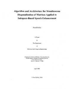
Composite Iterative Algorithm and Architecture for q-th Root Calculation
from RECP_LUT
13
from HR_LOG or Ex
Sj
1/q nd+gd
*
b
*
wm[j] +
Mult−Add K
nm+gm
j
Kj Recoding b
Tj
inria-00575573, version 1 - 10 Mar 2011
Kj−1
b
wm[j]
Tj
nm+gm
to on−the−fly_CONV or OL_HR_EXP
Figure 4: Block diagram of the LRCF multiplier. Since the fractional part is obtained with nl bits of accuracy, in the remaining iterations we compute Nl = dnl /be digits of the fractional part of T , which are used by the exponential unit without conversion. The total number of iterations of the LRCF multiplication is Nm = γ + Nl .
3.4
On-line high-radix exponential
The online high-radix algorithm for the computation of 2F is detailed in [12]. This algorithm is based on the identity P Y 2F = ( hj )2F − log2 (hj ) with hj = (1 + ej r−j ). The input operand F is only available up to the j + δ Pδ digit at iteration j, as F [0] = i=1 Fj r−j , with δ the online delay and Fj the digits of F . The recurrences for the residual and the exponential are given by: E[j + 1]
=
E[j](1 + ej r−j )
we [j + 1]
=
r(we [j] − rj log2 (1 + ej r−j ) + Fj+δ r−δ )
with j ≥ 1, E[1] = 1 and we [1] = rF [0]. The number of iterations required to obtain the exponential with ne bits of accuracy is Ne = dne /be. The block diagram of the exponential unit is shown in Fig. 5. We use selection by rounding to obtain the high-radix digits ej , with |ej | ≤ (r − 1), except for the first digit e1 , which is obtained by a lookup table. The lookup tables used in the first iteration are addresses one cycle in advance, since F [0] is known while F1+δ is being computed. The rounding is performed on an d estimate we [j + 1] obtained by truncating to t fractional bits the borrow-save residual we [j + 1]. RR n° 7564
14
Vázquez & Bruguera
F1 from the LRCF_mult b
b−bit CLA b+t
b+t
Round & recod.
TABLE e1 E[j]
BARREL SHIFTER
−ej log[(ne/2b)−1] b+1
b
e1 Mux−2 b+1
inria-00575573, version 1 - 10 Mar 2011
*
*
Mult−Add ne+ge
rE[j+1] ne+ge
ne+ge from the LRCF_mult
b+1
TABLE TABLE −ej /ln(2) −rj+1log (1+e j r−j)
b+1
ne+ge
r−j+1E[j]
1 and Mq ⊂ [0.5, 1), d1 is selected from the over-redundant digit set {−(2r − 1), . . . , 2r − 1} by table look-up. This table is addressed by the b + 2 most significant bits of Mq . The block diagram of this unit is shown in Fig. 8. A more detailed description of this unit can be found in [18].
RR n° 7564
18
Vázquez & Bruguera
from NORM_q
Mq nq
wd[j]
nd+gd
j
BARREL SHIFTER
b+t
Round & recod. d TABLE j b d1
b+2
d1
BSA 4:2
b
b+1
rwd[j]
b Mux−2 b+1
r−j+1wd[j] nd+gd nq
2(1−Mq)
*
b+1
nd+gd−b
nd+gd
nq
Mux−2 nd+gd
Mux−2 nd+gd
*
b
nd+gd−b
j
BARREL SHIFTER r−j+1D[j] nd+gd D[0]r −1 Mux−2 nd+gd
+
dj
*
Mult−Add
inria-00575573, version 1 - 10 Mar 2011
D[0]=1 b+1
*
rD[j]
Mux−2 nd+gd
+
Mult−Add nd+gd
wd[j] nd+gd
b+t
D[j]
nd+gd b
nd+gd−b
to OL_HR_mult Dj
Figure 8: Block diagram of the reciprocal unit.
4.2
Enhanced LZD and signed-digit shifter
Since S = Ex +log2 (Mx ) is obtained in the form of a sequence of γ +Nl radix-2b digits, the multiplication S ∗ = S × 2−Eq can only be performed as a digit right shift of S when Eq is an integer multiple of b. A more general solution is to decompose Eq in two terms as Eq = bEq /bc × b + Eq %b so that the operation is computed as a compound right shift of bEq /bc radix-r digits plus Eq %b bits. Provided that the maximally redundant radix-r digits Si are represented in a borrow-save (or carry-save) form and the radix is an integer power of 2 (r = 2b ), the right shift of Eq %b bits can be implemented as a regular binary shift 1 . The serial architecture proposed is shown in Fig. 9. The unit processes a digit S ∗ i per cycle (0 ≤ i < Ns ). First, a right shift of Eq %b < b bits is performed over Sj (−γ < j < Nl ) using two barrel shifters of 2b bits. Since this binary shift crosses the digit boundaries, the previous input digit Sj−1 is latched and then concatenated at cycle i to the left of Sj . The initial value of this latch is 0. The b most significant bits of the two barrel shifter output are passed to a level of latched 2:1 multiplexers controlled by a signal2 rsa = bEq /bc < Ns . This signal represents the number of radix-r digit shifted to the right in a hot-one code. The output of the barrel shifters is stored in the latch which corresponds to the number of shifted positions counted from the right (from 1 That 2 This
bits ns .
is, a bit shifted out to the right of a radix-r digit halves its value. bound is ensured by error analysis, so that S ∗ is computed with enough precision
INRIA
Composite Iterative Algorithm and Architecture for q-th Root Calculation
Sj
b
b
Sj−1 b
Eq%b
19
2b−bit barrel shifters>> log2(b)
0 rsa Ns−1 1
b
b
0 Mux−2 1 b
1
b
b 1
0 Mux−2 1
b
0 Mux−2 1
b
rsa 0
0 Mux−2 1
1
b
b
b
inria-00575573, version 1 - 10 Mar 2011
S*j
Figure 9: Block diagram of the serial signed-digit shifter. q
Example: n=16 b=4 q
nq
q= 0000100101001111 Prefix Tree of OR gates OR= 0000011111111111 not(OR)= 1111100000000000
q
f= 0000100000000000
f0
0
q
1
q
n q−1
fn q−2
f1
Hot−one code
lz=q 4 (0100) rsa= 3 (00010) E%b = 0 (00) q
qn −2
q
f0
Binary encoder
log (nq) 2 lz q
nq
fn −1 q
fn −1 q
Hot−one code radix−r encoder
mod(b) encoder
Ns rsa
log (b) 2 E%b q
Figure 10: Enhanced leading zero detector. Ns − 1 to 0). The latch outputs are shifted one radix-r digit to the right each cycle, while Si∗ corresponds to the value stored in the rightmost latch. The shifting amounts signals rsa and Eq %b are obtained with a slight modification of the decoding logic in the LZD using the relation Eq = nq − lzq . The architecture of this enhanced LZD is shown in Fig. 10. First, a hotone code string f0 . . . f1 f2 fnq −1 indicating the position of the leading one of Pnq −1 q = i=0 qi 2nq −1−i is obtained using a tree of OR gates (prefix tree, carry lookahead...) and a level of AND-2 gates with an inverted input. These signals are computed as i−1 fi = qi · ORj=0 qj Then, lzq , rsa = bEq /bc and Eq %b are computed as nq −1
lzq
=
X
i × fi
i=0 nq −1
rsa =
X i=0
RR n° 7564
b(nq − i)/bc × fi
20
Vázquez & Bruguera
nq −1
(Eq %b)
=
X
(nq − i)mod(b) × fi
i=0
with an appropriate decoding of the hot-one code signals fi using OR gates. Namely, the signal lzq is decoded to a binary operand of dlog2 nq e bits width, the signal rsa into a hot-one radix-r operand of Ns bits width, and the signal Ns into a binary (modulo b) operand of dlog2 be bits width. We show a toy example for nq = 16 q = 2383 and b = 4 (radix-16) in the left side of Fig. 10. We obtain lzq = 4, rsa = 3 and (Eq %b) = 0 as follows:
inria-00575573, version 1 - 10 Mar 2011
1. We compute signals f0 to f15 using the prefix tree of OR gates (dlog2 (16)e1=3 levels of two-input gates), and the level of NOT-AND2 gates, obtaining f4 = 1. 2. We obtain lzq = 4 (01002 ) from the binary encoder, implemented using the following boolean expressions: lzq (3)
= f8 ∨ f9 ∨ f10 ∨ f11 ∨ f12 ∨ f13 ∨ f14 ∨ f15
lzq (2)
= f4 ∨ f5 ∨ f6 ∨ f7 ∨ f12 ∨ f13 ∨ f14 ∨ f15
lzq (1)
= f2 ∨ f3 ∨ f5 ∨ f7 ∨ f10 ∨ f11 ∨ f14 ∨ f15
lzq (0)
= f1 ∨ f3 ∨ f5 ∨ f7 ∨ f9 ∨ f11 ∨ f13 ∨ f15
3. The hot-one code radix-16 encoder computes the value rsa = b(16 − lzq )/4c ∈ [0, 4] , producing an output rsa = 3 expressed in a hot-one code (00010). The logical expressions of this block are given by rsa(4)
= f0
rsa(3)
= f1 ∨ f2 ∨ f3 ∨ f4
rsa(2)
= f5 ∨ f6 ∨ f7 ∨ f8
rsa(1)
= f9 ∨ f10 ∨ f11 ∨ f12
rsa(0)
= f13 ∨ f14 ∨ f15
4. The modulo b=4 encoder produces a binary string of log2 (4) = 2 bits which represents the value (16 − lzq )%4 ∈ [0, 3]. The logical expressions of this block are given by Eq %4(1)
=
f1 ∨ f2 ∨ f5 ∨ f6 ∨ f9 ∨ f10 ∨ f13 ∨ f14
Eq %4(0)
=
f1 ∨ f3 ∨ f5 ∨ f7 ∨ f9 ∨ f11 ∨ f13 ∨ f15
For the example of Fig. 10, since lzq = 4, then f4 = 1 and (16−lzq )%4 = 0.
4.3
On-line multiplier
On-line multiplication [17] of P = X × Y is defined by the following recurrence equation for the scaled partial product wm [j] = rj X[j]Y [j]: wm [j + 1] = r(wm [j] − Pj ) + r−δ (Xj+δ+1 Y [j] + Yj+δ+1 X[j + 1])
(10)
Pj+δ Pj+δ −i −i with δ = 2 for r > 2, X[j] = i=1 Xi r , Y [j] = i=1 Yi r . The initial condition for the algorithm is wm [0] = X[0] × Y [0] and P0 = 0, where the INRIA
Composite Iterative Algorithm and Architecture for q-th Root Calculation
21
product digits Pj ⊂ {−(r − 1) . . . , 0, . . . , r − 1} are obtained in our case by a selection function Pj+1 = round(wmd [j + 1]), with wm [j + 1] truncated to t bits. After iteration j ≥ 0, the product is given by P = P [j + 1] + (wm [j + 1] − Pj+1 )r−j−1 with P [j + 1] = conditions:
Pj+1 i=1
Pi r−i . For convergence we have to verify the following
• General condition of convergence for the iteration: |wm [j + 1] − Pj+1 | ≤ ri+1 (P − P [j + 1]). Since |Pj | ≤ (r − 1), and P − P [j + 1] ≤
∞ X
(r − 1)r−i ≤ r−j−1
inria-00575573, version 1 - 10 Mar 2011
i=j+2
this condition can be formulated as |wm [j + 1]| ≤ (r − 1) + ri+1 r−j−1 , that is |wm [j + 1]| ≤ r. • Condition of convergence for selection by rounding: |wm [j + 1]| < (r − 1) + 1/2, that is |wm [j + 1]| < r − 1/2. To obtain upper bounds for the values of X and Y we check the second condition (more restrictive) for j = 0 . The scaled partial product wm [1] given by recurrence (10) with j = 0 can be expressed as wm [1]
= rwm [0] + r−δ (Xδ+1 Y [0] + Yδ+1 X[1]) = r(X[0]Y [0]) + r−δ (Xδ+1 Y [0] + Yδ+1 X[1]) = Y [0]r(X[0] + Xδ+1 r−δ−1 ) + X[1]r(Yδ+1 r−δ−1 ) = rY [0]X[1] + X[1]r(Yδ+1 r−δ−1 ) = rX[1](Y [0] + Yδ+1 r−δ−1 ) = rX[1]Y [1] (11)
Using r|X[1]Y [1]| ≤ r(|X × Y |) in the previous expression, the condition of convergence for selection by rounding limits the values of the input operands to |X × Y | < 1 − 1/2r To obtain a value for the minimum number of fractional bits t required for the estimate wmd [j + 1], we use the condition of convergence |wm [j +1]| < r−1/2 for j > 0. In this case, a bound for wm [j + 1] is given by wm [j + 1] ≤ r(1/2 + 2−t ) + r−δ 2(r − 1)(1 − 1/2r)1/2
(12)
obtained by introducing the following bounds in expression (10): |wm [j] − Pj | ≤ 1/2 + 2−t , |Xj+δ+1 | ≤ (r − 1), |Yj+δ+1 | ≤ (r − 1), |Y [j − 1]| ≤ (1 − 1/2r)1/2 , and |X[j]| ≤ (1 − 1/2r)1/2 . With the previous bound for |wm [j +1]|, the condition of convergence results in r(1/2 + 2−t ) + r−δ 2(r − 1)(1 − 1/2r)1/2 < r − 1/2 (13) obtaining a minimum value of t = 1 for r ≥ 4 and δ = 2. RR n° 7564
22
Vázquez & Bruguera
from SD_SHIFTER
from HR_RECP
Dj
S*j b
b
S*[j]
D[j]
Mux−2
S*[j+1] D[j+1]
Mux−2 nd+gd
ns+gs
nd+gd
Mux−2
inria-00575573, version 1 - 10 Mar 2011
nm+gm
+
*
*
*
*
Mult−Add
−rTj +
Mult−Add
nm+gm
nm+gm
rwm[j]
BSA 4:2 wm[0]
wm[j+1]
b+t
nm+gm
Mux−2 nm+gm
Round & recod.
Tj+1
nm+gm
b b
to on−the−fly_CONV or OL_HR_EXP Tj
Figure 11: Block diagram of the on-line multiplier. We perform the operation T = D × S ∗ using the online multiplier of Fig. Pd(n +g )/be 11. Since operands D and S ∗ are of the form D = i=0d d Di r−i with P P dn /be−1 d(n +g )/be Ex D0 = 1, and S ∗ = S ∗ i ri + i=1s s S ∗ i r−i , they need to be i=0 scaled by a constant to verify X × Y < 1 − 1/2r. Thus, we scale both operands as follows, X = Dr−1 (X1 = 1), and Y = S ∗ r−dnEx /be , so that X ×Y ≥ 2/r and X ×Y < 1−1/2r is verified for r ≥ 4. The product is given by T = P rdnEx /be+1 . We need an initial cycle to compute wm [0] = D[0]S ∗ [0] = S ∗ [0] + D1 S ∗ [0], and Nm = γ + Nl iterations of the recurrence (10) followed by the selection of Pj+1 = round(wmd [j + 1]) to get an accuracy of nm bits (nEx integer, nl fractional) of the product T .
5
Evaluation and Comparison
In this Section, we present estimates of the execution time and hardware cost for the proposed low and high precision q architectures described in Section 3 and 4. First, we describe the evaluation model used to obtain the area and delay estimates. Next, we particularize for single (n = 24, nEx = 8) and double precision (n = 53, nEx = 11) formats with radix values r = 2b ranging from r = 8 to r = 1024. Finally, we present a comparison with other representative implementations in Section 5.1.
INRIA
23
Composite Iterative Algorithm and Architecture for q-th Root Calculation
Component Nand2 Xor2 FA 1-bit 4:2 CSA 4-bit CLA 1-bit D-latch
Delay (F O4) 0.7 1.3 3.2 5 5.5 2.5
Area (NAND2) 1 2.5 7.5 15 35 3.5
Table 5: Area and delay values for CMOS components. nq 6 7 8 9 10 Single Precision (n, nEx )=(24,8) 1.12 2.25 4.5 9 18 36 335 675 1180 2360 4725 9450 6.4 8 9.6 11.2 12.8 14.4 Double Precision (n, nEx ) =(53, 11) 2.12 4.25 8.5 17 34 68 635 1275 2230 4460 8925 17850 6.4 8 9.6 11.2 12.8 14.4
inria-00575573, version 1 - 10 Mar 2011
5
Size (Kbits) Area (]Nand2) Delay (]FO4) Size (Kbits) Area (]Nand2) Delay (]FO4)
11
12
72 18900 14.4
144 32400 16
136 35700 14.4
272 61200 16
Table 6: Size, area and delay of look-up tables for reciprocal computation We use an area and delay evaluation model based on a simplification logical effort method [14] that allows for faster hand calculations. It considers the different input and output gate loads, but neither interconnections nor gate sizing optimizations. Instead, we use other optimization techniques, such as buffering or cloning (gate replication) to drive high loads. The total stage delay is obtained as the sum of the delays of the gates on the critical path. The delays are expressed in FO4 units (delay of an 1x inverter with a fanout of 4 inverters), and the area in number of equivalent minimum size NAND2 gates. We do not expect this rough model to give very precise area-delay figures, but it provides good first-order area and delay estimations to be used in technologyindependent comparisons. In Table 5 we detail the delay and area of some common CMOS gates and logic components. The hardware complexity and delay figures for look-up tables shown in Table 6 were extracted from synthesis evaluations as in [12] (see Apendix A in [11] for more details). Tables 7 and 8 show estimates of the latency (in number of cycles), cycle time and execution time (in FO4 units) of the q-th root computation, area of the high radix-r logarithm and on–line exponential units (in NAND2 units), and total area of the proposed low precision q architecture with nq = 8, for single and double precision computations respectively. The implemented radix values go from r = 8 to r = 1024. The latency of a q–root computation for the low precision q implementation was calculated in accordance with the formula 2 + γ + δ + Ne , with γ = 2 and δ = 2. The cycle time corresponds to the critical path delay of the logarithm unit, and is the sum of the delays of the round unit, a multiplexer and the RR n° 7564
24
Radix 8 16 32 64 128 256 512 1024
Vázquez & Bruguera
Latency (]cycles) 16 13 12 11 10 9 8 8
Cycle T. (]FO4) 30 32 32 34 34 36 36 37
Exec. T. (]FO4) 480 416 384 374 340 324 288 296
LOG Area (NAND2) 4500 5700 6600 9000 11400 18700 32600 60500
Exp. Area (NAND2) 4200 5400 6200 8500 10800 17600 30700 57000
Total Area (NAND2) 13650 16450 18200 23300 28250 42800 69900 124650
Table 7: Area and delay of the low precision q architecture with nq = 8 and single
inria-00575573, version 1 - 10 Mar 2011
precision (n = 24, nEx = 8).
Radix 8 16 32 64 128 256 512 1024
Latency (]cycles) 27 21 18 16 14 13 13 12
Cycle T. (]FO4) 31 33 33 34 34 36 36 37
Exec. T. (]FO4) 837 693 594 544 476 468 468 444
LOG Area (NAND2) 11350 12700 18100 20600 32900 58000 98000 133300
Exp. Area (NAND2) 11000 12300 17500 20000 31800 56100 94800 129100
Total Area (NAND2) 31400 34800 45700 51400 75700 125800 204800 275200
Table 8: Area and delay of the low precision q architecture with nq = 8 and double precision (n = 53, nEx = 11).
multiply-add unit. The main contribution to the total area of the q-root unit comes from both the high-radix logarithm and on–line exponential units, and this is significantly high for radix values r > 128. In addition, we observe that, very little advantage in execution time is obtained from using very high radix values (over r = 128). On the other hand, the estimated area look–up table for the reciprocal with nq = 8 is only 2360 NAND2 gates for single precision and 4460 NAND2 gates for double precision. However, as we show later, for higher precision values of q, such as nq > 10, the contribution of this look–up table to the total area is very significant, and the use of a look–up table to compute the reciprocal may be not justified. Tables 9 and 10 show the corresponding estimates for the high–precision q architecture, with nq = 32 and nq = 64 for the single and double precision computations respectively. In addition to the previous estimates, we show the area of the reciprocal unit for the different radix values. We include in this area estimation the fixed point high-radix iterative unit, the leading zero detector and the related shifters. The contribution of this unit to the total area is more significant in percentage for low radix values. Thus, for a given radix, the area of this architecture is higher than the area of the low precision q architecture for nq . Besides, there is a latency overhead of 3 cycles. On the other hand, a variation in the precision nq has a negligible impact on the total area or execution time. INRIA
Composite Iterative Algorithm and Architecture for q-th Root Calculation
Radix 8 16 32 64 128 256 512 1024
Latency (]cycles) 19 16 15 14 13 12 11 11
Cycle T. (]FO4) 30 32 32 34 34 36 36 37
Exec. T. (]FO4) 570 512 480 476 442 432 396 407
Recip. 6200 7050 7500 8700 9700 12000 15100 20650
25
Area (NAND2) Log. Exp. Total 4500 4200 21100 5700 5400 25200 6600 6200 27700 9000 8500 34400 11400 10800 40500 18700 17600 57800 32600 30700 88400 60500 57000 149100
Table 9: Area and delay of the high precision q architecture with nq = 32 and single
inria-00575573, version 1 - 10 Mar 2011
precision (n = 24, nEx = 8).
Radix 8 16 32 64 128 256 512 1024
Latency (]cycles) 30 24 21 19 17 16 16 15
Cycle T. (]FO4) 31 33 33 34 34 36 36 37
Exec. T. (]FO4) 930 792 693 646 578 576 576 555
Recip. 11200 12500 13200 15000 16200 18800 22300 28500
Area (NAND2) Log. Exp. 11350 11000 12700 12300 18100 17500 20600 20000 32900 31800 58000 56100 98000 94800 133300 129100
Total 44700 50250 62100 70400 96100 149700 232500 310000
Table 10: Area and delay of the high precision q architecture with nq = 64 and double precision (n = 53, nEx = 11).
Thus, we want to determine a threshold value for nq such that the high precision q architecture presents a hardware cost advantage over the low precision q architecture. We present in Table 11 area estimations of the low precision q architecture, for single and double precision computations, and for different values of nq from 5 up to 12. We choose a radix r = 128 since it seems to be the most advantageous in terms of the product execution time ×area. We also present the area estimations for the high-precision architecture for a radix value r = 128. We observe that for both single and double precision computations, the area of the low precision q architecture with nq = 11 is slightly higher than the area of the higher precision q architecture, although the latency is 3 cycles lower.
5.1
Comparison
The comparison of our q-th root computation method with previous alternatives is not easy. As far as we know, no other previously proposed algorithm and architecture, but a naive implementation of X 1/q = 2(1/q) log2 (X) and the extension of the powering architecture in [12], allows the computation of the q-th root for any value of q; that is, the other architectures in the literature are derived for a given value of q and changing q implies making a different implementation. On the contrary, the proposed architecture allows the computation RR n° 7564
26
Vázquez & Bruguera
inria-00575573, version 1 - 10 Mar 2011
q-th root unit with reciprocal by lookup table: Area (]NAND2) Single precision (n = 24, nEx = 8, 10 cycles latency) nq 5 6 7 8 9 10 11 12 Recip. 335 675 1180 2360 4725 9450 18900 32400 Total 26200 26600 27100 28250 30600 35350 44800 58300 Double precision (n = 53, nEx = 11, 14 cycles latency) nq 5 6 7 8 9 10 11 12 Recip. 635 1275 2230 4460 8925 17850 35700 61200 Total 71900 72500 73500 75700 80200 89100 107000 132500 q-th root unit with reciprocal by high-radix digit-recurrence Latency (cycles) Area 1/q (NAND2) Total Area (NAND2) SP 13 10850 40500 DP 17 18600 96100
Table 11: Determining the best unit in terms of cost for r = 128 as a function of nq . SP (n=24, nEx =8, nq =32), DP (n=53, nEx =11, nq =64).
of any q–th root without any additional modification. It has to be pointed out that the complexity of the extended algorithm in [12] which implements Equation (3), makes it very hard and inefficient to implement more than a small set of q–th roots. Basically, there are two types of algorithms for the computation of the q-th root. Algorithms based on table-driven polynomial approximations [2, 10, 15] and digit–recurrence algorithms [8]. Among the former, in [15] a method for generating X p for a given p is proposed, applicable to values of p = ±2k or p = ±2k1 ± 2k2 being k1 an integer and k2 a non-negative integer. This includes a limited number of roots, such as square root, fourth root, eighth root, etc. The powering function is computed by a piecewise linear approximation based on modified first–order Taylor expansion. The first–order Taylor expansion is rewritten as X p = C × X 0 being X 0 = X1 + 2−m−1 + p × (X2 − 2−m−1 ), and X1 and X2 the upper m-bit part and the lower part of X, respectively. C can be read through a table look-up addressed by X1 and, for special p’s, X 0 is easily obtained by modifying X. Only one multiplication is required to evaluate the modified Taylor expansion. A second–order minimax approximation is presented in [10], which allows the computation of X p for any given p. This includes every q-th root. X p is approximated as C2 × X22 + C1 × X2 + C0 . The three coefficients C2 , C1 and C0 are stored in look–up tables and selected by X1 . The size of the tables is optimized by carefully minimizing the coefficients wordlength for the required precision. The evaluation of the powering requires, besides the look–up tables, a squaring unit and a fused accumulation tree. Another second–order interpolation for the evaluation of elementary functions, including q-th roots, is presented in [2]. The table sizes are reduced by storing the function values and one coefficient for each interpolation subinterval, instead of storing all the three coefficients as in the proposal above. The two remaining coefficients are computed from the function values. This way, the memory requirements are reduced by one third. Additionally, some multipliers and adders are need to complete the powering computation.
INRIA
Composite Iterative Algorithm and Architecture for q-th Root Calculation
Latency cycle time Delay (cycles) (FO4) (FO4) Composite LOG-MUL-EXP Algorithms (r = 128) Our architecture (nq = 8) 10 34 340 Our architecture (nq = 32) 13 34 442 Naive (nq = 8) 15 34 510 X p with p integer [12] 9 34 306 X 1/q (nq = 8) [12] 9 34 306 Linear approx. [15] 1 51 51 2nd–order interp. [10] 3 18.7 56.1 2nd–order interp. [2] 2 54.4 108.8 Digit–recurr. (q = 3, r = 2) [13] 52 119 6188
inria-00575573, version 1 - 10 Mar 2011
Architecture
27
Area (NAND2) 28250 40500 33015 29827 > 500000 26122 10170 10612 9035
Table 12: Architecture features comparison for single–precision floating–point representation and low precision q.
Note that the three algorithms and architectures above for the computation of X 1/q are targeted for a given q. To adapt the architecture to other different q, when possible, requires changing the look–up tables. On the other hand, a general digit–recurrence algorithm for the computation of the q-th root has been presented in [8]. The result is a general algorithm that must be particularized for each different q, and the larger q the larger the complexity. This general algorithm has been used to implement a cube root unit [13]. In order to evaluate our architecture, we compare the algorithms based on a table-driven polynomial approximation and the digit–recurrence algorithm outlined above. However, it has to be kept in perspective that, unlike our algorithm, all these algorithms have to be particularized for a given q when implementing the q-th root unit. Moreover, we include in the comparison the naive implementation of X 1/q = e(1/q)ln(X) and the architecture for the computation of X p and its extension to X 1/q , with p and q integers, presented in [12]. Table 12 shows the latency, delay and area estimate of every algorithm and implementation. We have considered a single–precision floating–point representation for X and low–precision q; in particular, we consider nq = 8 for low precision q and nq = 32 for our architecture with higher precision q. For the architectures based on composite logarithm-multiplication-exponential algorithms, we have used a radix r = 128. As shown in Tables 7-10, a good tradeoff between latency, cycle time and area can be achieved for specific values of the radix. Although it is difficult to select just one radix for every implementation, in applications demanding high-speed processing one of the most efficient implementations corresponds to radix r = 128. Note that, although the table-driven polynomial approximation are implemented for a given root, the latency, delay and area are roughly the same for any root. However, the features of the digit–recurrence architecture are closely related to the value of q; so, we show the features for the computation of the radix 2 cube root described in [13].
RR n° 7564
inria-00575573, version 1 - 10 Mar 2011
28
Vázquez & Bruguera
As expected, the latency, total delay and area of the table–driven polynomial approximation architectures is significantly smaller than in the architecture we have proposed in this paper, because those architectures can compute only a given root. Of course, those architectures could be extended to compute more than just one given root. This means that tables to store the coefficients or the function values need to be replicated to include one set of tables for each root. This affects the total area and the cycle time. Similarly, the digit–recurrence architecture is tailored to a given root, as well. The computation of a different root implies the development of completely different architecture. The larger the q the larger the complexity. Finally, the features of our architecture and the architecture in [12] are quite similar. Both architectures are based on similar optimizations of the naive implementation of X 1/q = 2(1/q) log2 (X) ; however, the extension of the architecture in [12] to the computation of a q-th root, is quite inefficient. This is mainly due to the huge table required to obtain 2(Ex %q)/q once the modulus of the integer division Ex %q has been evaluated, even for low precision q.
6
Conclusion
An algorithm for q–th root extraction has been presented, based on a high– radix composite algorithm. It consists of computing X 1/q as 2(1/q)×(Ex +log2 (Mx )) through a sequence of parallel and /or overlapped operations: reciprocal, high– radix digit–recurrence logarithm, high–radix left–to–right carry–free multiplication and on–line high–radix exponential. A detailed error analysis has been carried out to determine the intermediate wordlengths. The algorithm is based on a previous algorithm for the computation of the powering function X p , with p any integer, which was extended for the computation of q–th roots. However, the extended algorithm seems hard to implement since it is necessary to compute an integer division and a modulus operation. Our algorithm avoids these two operations, resulting in a much simpler algorithm. Two architectures have been proposed. First, an architecture for low precision q values, less than 12 bits, where the reciprocal 1/q is obtained directly from a look–up table; after that, an alternative architecture for higher precision values of q, where a high–radix iterative algorithm has been used for the computation of the reciprocal. Both architectures have been evaluated and estimates of the execution time, the latency and the area have been obtained, based on an approximated model for the delay and the area of the main building blocks, for single and double precision floating–point representations and several radices. The analysis of the tradeoffs between area and speed allows us to determine the better radix for every implementation: radix r = 128 might be suitable for high speed implementations. Larger radices result in similar execution times with much larger area requirements. The comparison with other previous algorithms is not easy. As far as we know, no other previously proposed methods, except the extension of the architecture for the computation of X p , allow the computation of the q–th root for any value of q. Even so, we have discussed the area and time figures for several non–general implementations for q–th root calculation and the powering architecture to determine the suitability of our implementation. The conclusion INRIA
Composite Iterative Algorithm and Architecture for q-th Root Calculation
29
is that the execution times and hardware requirements are better than those of the powering function calculation and, although obviously are worse than those of the non–general q–th root extraction architectures, the flexibility of our implementation makes it an interesting alternative. Work is in progress to integrate the proposed q–th root computation with the previous powering function algorithm into a combined unit which would be able to compute any function of type X p/q .
References
inria-00575573, version 1 - 10 Mar 2011
[1] J. Cao and B.W.Y Wei, High-performance hardware for function generation, Proc. 13th IEEE Symposium on Computer Arithmetic, pp.184–188, Jul. 1997. [2] J. Cao, B. W. Y. Wei and J. Cheng, High-performance architectures for elementary function generation, Proc. 15th IEEE Symposium on Computer Arithmetic, pp. 136–144, Jun. 2001. [3] M. D. Ercegovac and T. Lang, Fast Multiplication Without Carry-Propagate Addition, IEEE Transactions on Computers, vol. 39 no. 11, pp. 1385–1390, Nov. 1990. [4] M.D. Ercegovac and T. Lang, On-the-Fly Rounding, IEEE Transactions on Computers, vol. 41, no. 12, pp. 1497–1503, Dec. 1992. [5] M.D. Ercegovac and T. Lang, Digital Arithmetic, Morgan Kaufmann, 2004. [6] M.D. Ercegovac, Digit-by-Digit Methods for Computing Certain Functions, 41st Asilomar Conference on Signals, Systems and Computers, pp. 338–342, Nov. 2007. [7] IEEE Std 754(TM)-2008, IEEE Standard for Floating-Point Arithmetic, IEEE Computer Society, Aug. 2008. [8] P. Montuschi, J.D. Bruguera, L. Ciminiera and J.-A. Piñeiro, A Digit-byDigit Algorithm for mth Root Extraction, IEEE Transactions on Computers, vol. 56, no. 12, pp. 1696–1706, Dec. 2007. [9] J.-M. Mueller, Elementary Functions, Algorithms and Implementation, Birkhäuser, 1997. [10] J.-A. Piñeiro, J.D. Bruguera and J.-M. Mueller, Faithful Powering Computation Using Table Lookup and Fused Accumulation Tree, Proc. 15th IEEE Symposium on Computer Arithmetic, pp. 40–47, Jun. 2001. [11] J.-A. Piñeiro, Algorithms and Architectures for Elementary Function Computation, Ph.D. Dissertation, Dept. of Electronics and Computer Engineering, University of Santiago de Compostela, Spain, Jun. 2003. Available at http://www.ac.usc.es. [12] J.-A. Piñeiro, M.D. Ercegovac and J.D. Bruguera, Algorithm and Architecture for Logarithm, Exponential and Powering Computation, IEEE Transactions on Computers, vol. 53, no. 9, pp. 1085–1096, Sep. 2004. RR n° 7564
30
Vázquez & Bruguera
[13] A. Piñeiro, J.D. Bruguera, F. Lamberti, P. Montuschi, A Radix-2 Digit-byDigit Architecture for Cube Root, IEEE Transactions on Computers, vol. 57, no. 4, pp. 562–566, Apr. 2008. [14] I.E. Sutherland, R.F. Sproull and D. Harris, Logical Effort: Designing Fast CMOS Circuits, Morgan Kaufmann, 1999. [15] N. Takagi, Powering by a Table Look-Up and a Multiplication with Operand Modification, IEEE Transactions on Computers, vol. 47, no. 11, pp. 1216– 1222, Nov. 1998.
inria-00575573, version 1 - 10 Mar 2011
[16] N. Takagi, A Digit-Recurrence Algorithm for Cube Rooting, IEICE Transactions on Fundamentals of Electronics, Communications and Computer Sciences, vol. E84-A, no. 5, pp. 1309–1314, May 2001. [17] K.S. Trivedi and M.D. Ercegovac, On-Line Algorithms for Division and Multiplication, IEEE Transactions on Computers, vol. C-26, no. 7, pp. 681– 687, Jul. 1977. [18] A. Vazquez, E. Antelo and T. Lang, Combined Division/SquareRoot/Reciprocal Square-Root Unit for 3D Graphics Geometry Processing, Tech. Report, Department of Electronic and Computer Science. University of Santiago de Compostela, Spain. Sep. 2000. Available at http://www.ac.usc.es.
INRIA
inria-00575573, version 1 - 10 Mar 2011
Centre de recherche INRIA Grenoble – Rhône-Alpes 655, avenue de l’Europe - 38334 Montbonnot Saint-Ismier (France) Centre de recherche INRIA Bordeaux – Sud Ouest : Domaine Universitaire - 351, cours de la Libération - 33405 Talence Cedex Centre de recherche INRIA Lille – Nord Europe : Parc Scientifique de la Haute Borne - 40, avenue Halley - 59650 Villeneuve d’Ascq Centre de recherche INRIA Nancy – Grand Est : LORIA, Technopôle de Nancy-Brabois - Campus scientifique 615, rue du Jardin Botanique - BP 101 - 54602 Villers-lès-Nancy Cedex Centre de recherche INRIA Paris – Rocquencourt : Domaine de Voluceau - Rocquencourt - BP 105 - 78153 Le Chesnay Cedex Centre de recherche INRIA Rennes – Bretagne Atlantique : IRISA, Campus universitaire de Beaulieu - 35042 Rennes Cedex Centre de recherche INRIA Saclay – Île-de-France : Parc Orsay Université - ZAC des Vignes : 4, rue Jacques Monod - 91893 Orsay Cedex Centre de recherche INRIA Sophia Antipolis – Méditerranée : 2004, route des Lucioles - BP 93 - 06902 Sophia Antipolis Cedex
Éditeur INRIA - Domaine de Voluceau - Rocquencourt, BP 105 - 78153 Le Chesnay Cedex (France)
http://www.inria.fr ISSN 0249-6399