NO. 3. MARCH 1991. 683. Compound Gauss-Markov Random Fields for Image. Estimation. Fure-Ching Jeng, Member, IEEE, and John W. Woods, Fellow, IEEE.
IEEE TRANSACTIONS ON SIGNAL PROCESSING, VOL. 39. NO. 3. MARCH 1991
683
Compound Gauss-Markov Random Fields for Image Estimation Fure-Ching Jeng, Member, IEEE, and John W. Woods, Fellow, IEEE
Abstmct-This paper is concerned with algorithms for obtaining approximations to statistically optimal estimates for images modeled as compound Gauss-Markov random fields. We consider both the maximum aposteriori probability (MAP) estimate and the minimum meansquared error (MMSE) estimate for both image estimation and image restoration. Compound image models consist of several submodels having different characteristics along with an underlying structure model which governs transitions between these image submodels. Compound Gauss-Markov field models can be attractive for image estimation because the resulting estimates do not suffer the oversmoothing of edges that usually occurs with Gaussian image models. Two different compound random field models are employed in this paper, the doubly stochastic Gaussian (DSG) random field and a newly defined compound Gauss-Markov (CGM) random field. We present MAP estimators for DSG and CGM random fields using simulated annealing, a powerful optimization method best suited to massively parallel processors. A fast converging algorithm called deterministic relaxation, which however converges to only a locally optimal MAP estimate, is also presented as an alternative for reducing computational loading on sequential machines. For comparison purposes, we also include results on the fixed-lag smoothing MMSE estimator for the DSG field and its suboptimal M-algorithm approximation. The incorporation of causal and nodcausal modeling together with causal and noncausal estimates on the same data sets allows meaningful visual comparisons to be made. We also include Wiener and reduced update Kalman filter (RUKF)estimates to allow visual comparison of the near optimal estimates based on c6mpound Gauss-Markov models to those based on simple Gaussian image models.
I. INTRODUCTION
A
S is well known, a linear-shift invariant (LSI) model is not well suited to image estimation, i.e., noise smoothing. The major problem is that the resulting image estimate suffers from oversmoothing of edges which are quite important to the human visual system (HVS). Partly as a result, space-variant filters have been proposed [ 11, [8], [ 121, [ 141 wherein each pixel (or block of pixels) is filtered by a switched linear filter with the switching governed by a visibility function. The visibility function can be based on either a local variance estimate [8] or an average estimate of the isotropic gradient [l]. A more complicated visibility function which depends upon the mix of the directional components and a high frequency component was used in [12]. One of the problems with all these approaches is that the filter switching is rather ad hoc and cannot be justified on a theoretical basis. It would be better if the filter transitions could be related to an image model. Manuscript received February 9, 1988; revised April 23, 1990. This work was supported by the National Science Foundation under Grant ECS8313880. F.-C. Jeng is with Bellcore, Monistown, NJ 07960, and was visiting at the Center for Automation Research, University of Maryland at College Park, College Park, MD 20742, while this work was being done. J. W.Woods is with the ECSE Department, Rensselaer Polytechnic Institute, Troy, NY 12180-3590. IEEE Log Number 904 1598.
One way to embed a mathematical approach into the above adaptive methods is to have the models’ switching controlled by a hidden random field. Toward this end, a class of models called compound Gauss-Markov models has been proposed [5], [15]. A compound random field consists of two levels, upper and lower. The upper level random field is the observed image, which is composed of several LSI submodels representing a variety of local characteristics of images, e.g., edge orientation or texture. The lower or hidden level is a random field with a finite range whose purpose is to govern transitions between the observed LSI submodels. The doubly stochastic Gaussian (DSG) field [ 151 possesses a conditional Gaussian, autoregressive (AR) upper or observed level, whose model coefficients have a causal support. They are switched by a hidden (hence lower level) 2-D causal Markov chain to generate the required local edge structure. The DSG random field is a Markov random field but the observed upper level component, by itself, is not, i.e., the image data component of the DSG is not Markov. In [15] a 2-D fixed-delay causal estimator called the M algorithm is presented for approximation to the minimum mean-squared error (MMSE) optimal estimate. Geman and Geman, on the other hand, used a noncausal neighborhood system in their image model [ 5 ] . In their nomenclature, our lower level random field becomes their line process which was defined on an interpixel grid system. Their upper level random field is a noncausal conditional Markov random field also with a finite range, i.e., a noncausal 2-D Markov chain. Since they modeled images on a finite range space, they thereby excluded the Gaussian models, which are very widely used in image estimation and restoration. Generalizing their model, we have introduced an extension of the Gauss-Markov random field [ 101, [ 171. Our compound Gauss-Markov (CGM) model [6] has continuous grey levels as an upper level observations model but retains the Gemans’ lower level line process (field) as a structural model. As mentioned above, both DSG and CGM models will be used in this paper, both for estimation and restoration. Their MAP estimators will be developed by means of simulated annealing (stochastic relaxation) which was first introduced by Geman and Geman [5] where they presented a convergence proof for this iterative method. Their proof was confined to images that are modeled by a finite range space which, unfortunately, excludes the case of CGM models. When applying simulated annealing to our models, a proof for the convergence of simulated annealing to the MAP estimate was thus lacking. We have obtained such a proof for a broad subclass of CGM models [7]. This paper will concentrate on the algorithm and experimental results of applying simulated annealing with CGM models to image estimation and restoration. Those interested in the more theoretical aspects of this work are referred to [7]. It is well known that simulated annealing is a computation-
1053-587X/91/0300-0683$01.00 0 1991 IEEE
684
IEEE TRANSACTIONS ON SIGNAL PROCESSING, VOL. 39, NO. 3, MARCH 1991
ally demanding method. Alternatively a quickly converging algorithm called deterministic relaxation can be used to get a local MAP estimate. This deterministic relaxation method has been called iterated conditional mode (ICM) in [2]. We also present results for this locally convergent algorithm. We start by defining the two compound random fields. Then estimation problems are formulated and the various estimators are briefly described. Next, we present simulation results that provide comparisons between the various methods, i.e., causal versus noncausal model, compound Gaussian versus simple Gaussian, noncausal MAP versus causal M-algorithm, and simulated annealing versus deterministic relaxation. The intent here will be to see which algorithms result in subjectively good images. We then draw conclusions about which mathematical models best match this human visual system (HVS) viewpoint.
Fig. 1. Coefficient support region 6t of the first-order model.
n) of S for which ( m , n ) E c,. In the above GM model, we have
11. COMPOUNDMARKOVRANDOMFIELDS As described in the Introduction, a simple shift-invariant Gaussian AR model can often lead to oversmoothing of image data. In this section, we will present two compound Markov models, the noncausal CGM and the causal DSG, that address this problem. A . Compound Gauss-Markov Random Fields
We can generalize the Gemans' compound model by incorporating a conditional Gauss-Markov observational model [lo], [17] with their line field, as indicated below. A simple GaussMarkov (GM) model can be described as follows:
s(m, n ) =
c
klscR
c k l s ( m- k, n - I )
+ w ( m , n)
(1)
A CGM model consists of several conditionally Gauss-Markov submodels with an underlying structure or line field. Here
(4) where w l ( m . n ) ( mn,) is a conditionally Gaussian noise whose variance controlled by the 1 ( m , n ) and 1 ( m , n ) is a vector which consists of four nearest neighbors of the line field surrounding the pixel s( m , n ) , with I ( m , n ) denoting the Geman's line field. This line field takes on two values indicating whether a bond is broken or not. If a bond is broken between adjacent pixels, then there is little covariance between them, otherwise, a strong covariance exists. The joint mixed probability density function (mpdf) of S, L is the Gibbs distribution
where w ( m , n ) is a Gaussian random field satisfying the following covariance constraint: where the constant Z, is independent of S, L. Also T i s a temperature parameter, U,is defined in (3), and U,is of the form if ( m , n) = ( k , I )
0
otherwise.
and 8 is shown in Fig. 1. A random field described by the above equation is a Markov random field with a neighborhood support 8 [lo], [17]. By the equivalence of Markov random fields and Gibbs distributions, we can write the joint probability density function (pdf) p (S) as the Gibbs pdf
e
I( i , j ), and where the N ' X N ' matrix L has elements I, where N" is the total number of points in the line field over the finite observation region. The clique system cI used in this paper is the same system used in [5] as shown in Fig. 2. For a CGM model to have a valid conditional Markov random field given a realization of the n): , line field L , there are covariance constraints on w ' ( m * n ) ( m
and
where c, is a clique, C , denotes the clique system for the given Markov neighborhood system, and Z, is a normalizing constant which is functionally independent of the matrix S, with elements sv s( i , j ). Each Vc$( S ) is a function on the sample ( S ) involves only those s ( m , space with the property . . . that Vc,
e
By commutativity of covariance of two random variables, we have the following constraint on the model coefficients:
JENG AND WOODS: COMPOUND GAUSS-MARKOV RANDOM FIELDS
0 0 0 0
0 0
010 0 0
vz2.7
v = I .I
0 0
I
v10.0
I I
0 0
010
vio.9
V118
55 55
685
010 010
I-
Vn2.7
Fig. 2. The clique system c,.
This constraint reduces the total number of free parameters that can be used in parameter identification. Consequently, classical unconstrained least squares parameter identification is not appropriate. Since the CGM model has a Gibbs probability distribution, it is a Markov random field. Depending on the functional U,(S 1 L), the hi&n random field L , by itself, may or may not be a Markov random field. This can be seen from the following expression for the probability function P( L ) :
If js e L ) / T dS has the form of Gibbs distribution for L , then L is a Markov random field, otherwise it is not. In general, e-”‘(‘IL)fTdS may not be a Gibbs distribution for L.
ss
B. Doubly Stochastic Gaussian Random Fields In the following, we will give a brief description of the DSG model. Before we describe this model, we need to introduce the 2-D causal Markov chain and a corresponding AR random ;field
~
1
.
Dejnition: The 2-D Markov chain 1 ( m , n ) is called a causal Markov chain if the following condition is satisfied:
where @ ,+ ( m , n ) is the local state support region shown in Fig. 3 and “ ( i , j ) < ( m ,n)” means “ i < m or i = m and j < n” which is consistent with progressive image scanning. In this paper. a 1 X 1 order Markov chain is used exclusively, i.e., @ , + ( r n , n ) = { ( m - 1 , n ) , ( m l , n - I), ( m , n l ) , ( m - 1 , n - 1 ) ) . Thus we can write
+
Fig. 3. Coefficient support regions @l.+(m, n ) ahd ( R e - ( m , n).
Dejnition: The random field s ( m , n ) is called a causal AR random field if it can be described by
where w( m, n ) i $ 8 bhite noise field and @ ,+ { (k,1 ): ( -k, -l)E@,+(O,O)}. We will use 1 x 1 order AR models exclusively in this paper. Dejnition: A random field s ( m , n ) is called a DSG random field [15] if it can be described as
where I ( m , n ) is a causal Markov chain and the submodel coefficients at ( m , n ) in general depend upon 1 ( m , n ) . The joint mpdf can be expressed as follows:
P(S9 L ) = P ( S 1 L ) W ) . Note that the formulation of the joint mpdf of the DSG model is different from the CGM model. It is easily seen that, by construction, the line field of the DSG model itself is a Markov random field. 111. ESTIMATORPROBLEMFORMULATIONS We wish to estimate the original image s ( m , n ) from the degraded observations r ( m , n ) on an N X N region:
where h ( k , 1 ) is a known point spread function (psf) with finite support region ahand v ( m , n ) is zero-mean, white noise independent of s ( m ,n ) and having variance U:,. In the following context, two criteria for estimation will be discussed. We briefly specify the minimum mean-square error (MMSE) criteria as used in the fixed-delay causal estimator for the DSG model from [ 151. Then we specify the maximum a posteriori probability (MAP) criteria as used in this work. Ultimately in Section VI, we will see some indication as to which estimation criteria is subjectively more relevant, i.e., which matches the HVS better. A . Fixed-Lag Minimum Mean-Square Error Estimate
The object is to find the fixed-lag minimum mean-squared error (MMSE) estimate of s ( m - k , n - 1 ) given the scanned set of all observations up to pixel ( m , n ) denoted
686
IEEE TRANSACTIONS ON SIGNAL PROCESSING, VOL. 39, NO. 3, MARCH 1991
where k, 1 represent fixed lag parameters (i.e., k 1 0, 1 I 0). Due to the generalized dhusal nature of the DSG random field, this fixed-lag criterion is quite suitable. It has the advantage of enabling the processing of scanned image data as it amves, i.e., without a frame store.
Then the MMSE estimate was written as
i [ ( m - k, n
i , [ ( m - k, n - l ) l ( m , n ) ]
C1
=
B. Maximum the A Posteriori Joint Density Estimate The a posteriori joint mpdf for S and L given R can be decomposed as
- l)l(m,n)]
L(n- I ) N + m
J=
P [ L J ( m ,n ) I R ( m n ) ]
where the aposteriori probability P [ L J ( m ,n ) l R ( m , n)] was given as
P [ L , ( m , n ) IR(m9
s
It can be seen that the MAP criteria leads to the need for a frame store to hold the entire image during processing. It also indirectly leads to iterative algorithms requiring massive parallelism for their efficient solution. Interestingly, neither error criteria is cleaFly more relevant to image processing. For example, the MMSE estimate should yield an estimate that is closest to the observed data on average. And the MAP criteria, while currently more popular than MMSE, may conceivably yield an estimated image that is most probable given the model, but still very unlikely given the data.
*
P[L,(m
- 1 , n ) ( R ( m - 1, n ) ]
with k a normalizing constant and lJ a local state for the hidden Markov chain l ( m , n ) . Notice that the number of terms in the summation in (14) grows exponentially. To reduce computation, we can keep a fixed number, say M , of paths at each pixel and discard the rest to control computations and storage space. 1) Suboptimal Solution: M-Algorithm: Instead of carrying forward the a posteriori probabilities P [ L J ( m ,n) I R ( m , n ) ] for all j, we now keep only the M most ptobable of the LM possible extensions and discard the rest. The M-algorithm can be formulated as follows: I
i [ ( m - k, n
- l ) ( ( m ,n ) ]
IV . ESTIMATOR SOLUTIONS In this section, we review a previousiy derived causal MMSE estimator for the DSG model and also present new noncausal MAP estimators [7] for both the CGM and DSG models. Then we present the suboptimal deterministic relaxation for the MAP estimate of both models.
n)]
- P [ r ( m , n ) ( R ( m - 1, n ) , L,(m, n ) ]
where the matrices S, L have been previously defined and R is defined as the N X N matrix with elements ru A r ( i , j ). Our object is to find the joint matrix estimate and t such that
(13)
41
= k P [ $ ( m , n ) l { ( m - 1,
(12)
p ( s , L I R ) = maxp(S, L I R ) . s,L
(14)
=
c i , [ ( m - k, n - l ) l ( m , n ) ] - P [ L J ( m ,n ) IR(m, n ) ]
J=l
where the a posteriori probabilities are given by
A. Optimal MMSE Estimates An optimal MMSE solution for the DSG model was derived in [15]. Using their notation, let L j ( m , n) be thejth submodel sequence and lj ( m , n ) be the value of this sequence at the pixel ( m , n). Then
with j = 1 , 2,
~~~~~
For the jth sequence, they wrote
Jj[(m - k, n
p
- I ) ( ( m .n ) ]
E [ s ( m - k, n
- l ) I R ( m , n), L j ( m , n)].
-
, M and k ( m , n ) a normalizing constant.
~
~~~
B. Joint MAP Estimator-Simulated Annealing Approach Since the criterion function p (S, L I R ) is nonli?ear, it is extremely difficult to find the optimum solutions, $, L by any conventional method. In [ 5 ] , a relaxation technique, called sto-
JENG AND WOODS: COMPOUND GAUSS-MARKOV RANDOM FIELDS ‘
chastic relaxation or simulated annealing, is developed to search for MAP estimates from degraded observations. In the following, we will present a variation of simulated annealing appropriate for both CGM and DSG models. Assume that s ( m , n ) is either a CGM or a DSG random field and the observations r ( m , n ) satisfy (11). Some notation is first
601
defined for the sake of conciseness: S(m,n)
L(m,n)
’ ’{
{ s ( k , I ) : v(k, I )
l ( k , I ) : v(k, 1 )
* ( m , .)} + (m,
A ) CGM Case: The conditional a posteriori density function a s ( m , n ) for s ( m , n ) given S ( m , n )L, a n d R is
where Z3 is a normalizing constant. The conditional aposteriori probability function a ’ ( m , n ) for I ( m , n ) given L,,,,), S a n d R is
where 1 (m,n ) is located between the two neighboring pixels s ( i , j ), s ( i ’ , j ’ ) and
’
s ( ~ , ~ ) , ( ~ ‘ {s(k, .~‘)
1 ) : v ( ~ , Iz) ( i , j ) o r ( i ’ , j ’ ) } .
The dependence o f p ( s ( i , j ) , s ( i ‘ , j ‘ ) I L ) P ( L on ) I ( m , n ) can be determined from (5). In fact, a ‘ ( m , n ) can be explicitly written as follows:
where Z4 is a normalizing constant.
688
IEEE TRANSACTIONS ON SIGNAL PROCESSING.
VOL. 39,
NO. 3, MARCH 1991
B) DSG Case: The conditional a posteriori density function us(mrn ) for s ( m , n ) given S(m,n)rL and R is
a ( m , n ) = p [ s ( m , n ) l S ( m , n ) * L, R ] s(i,j) 1 = -5e x p i -
( i ,j ) E ( R e - ( m , n )
r(m
-c
UEmh
+ i, n
-
((
+ j )
cLji.J)s(i- k , j
-
2 Tdv,C,.,,
-
c
h,,s(m
klEmh
+ i - k, n + j
-1)
\
where Z5 is a normalizing constant and the support region B e- ( m , n ) is specified in Fig. 3. The conditional aposteriori probability function *'(in, n ) for l ( m , n ) given L ( m , n )S, and R is ~ ' ( mn,) = P [ l ( m , n ) IL(m,n),S, R ]
(or iteration) of the image. Since r s ( m , n ) and ~ ' ( mn ,) both depend on T, we henceforth denote them by r:( m , n ) and rf(m , n ) , respectively. 1 ) Sequential Simulated Annealing Algorithm: The sequential simulated annealing algorithm can be described as follows: Let (m,, n , ) , t = 1, 2, * , be the sequence in which the sites are visited for updating.
--
Set t = 0 and assign an initial configuration denoted as S- I , L - and an initial temperature T ( 0) = 1. The evolution L, - I -+ L, of the hidden system can be obtained by sampling the next point of the hidden system from the raster-scanning scheme based on the conditional probability mass function r:( m,, n,) and keeping the rest of L, unchanged. Set t = t 1. Go back to step 2 until a complete sweep of the field L is finished. The evolution S, - I + S, of the observed system can be obtained by sampling the new value of the observations s ( m , , n,) based on the conditional pdf r s ( m , , n , ) and keeping the rest of S,- I unchanged. 1. Go back to step 4 until a complete sweep Set t = t of the whole image is achieved. Go to step 2 until t >,,t where t,is a specified integer.
-,
+
+
Inserting these two equations into (17), we have
The following theorem from [7] guarantees that simulated annealing converges to the MAP estimate if the stated conditions are satisfied. Theorem 1: If the following conditions are satisfied:
~1 a) CkI IciII = p < 1 b) Let T ( r ) 0 as t 00, and c) T ( t ) 2 C / l o g ( 1 + k ( t ) ) , -+
+
then f o r any starting conjguration S- I , L p(S,, L,(S-,, L - I ,R )
s(m, n ) -
c c i $ m * n ) s ( m- k, n - 1 )
The simulated annealing method can be implemented in a se-. quential or parallel manner. We first describe sequential simulated annealing, which is appropriate for raster scanning of the image. We keep the temperature constant for each sweep of the image and reduce the temperature only after the complete sweep
+
ro(S, L ) ,
I,
we have as t
+
00
(19)
where ro( * , * ) is the uniform distribution over the MAP solutions and k ( t ) is the sweep iteration number at time t . 2 ) Parallel Simulated Annealing Algorithm: As pointed out in [ 5 ] , [ l l ] , stochastic relaxation converges very slowly to the MAP estimate because of the logarithmic temperature cooling schedule. Now, in [5], it was suggested that simulated annealing can be implemented in a? asynchronous parallel machine to speed up the processing. However, an asynchronous machine may be rather difficult to implement and use compared to a single-instruction multiple-data (SIMD) machine. Here we present a coding scheme for implementation of simulated annealing on an SIMD machine as has been suggested by Murray et al. in [13], [4]. The total speed-up depends on the size of the neigh-
JENG AND WOODS: COMPOUND GAUSS-MARKOV RANDOM FIELDS
borhood of the Markov random field. In theory, we can have 2N2/k speed-up if we have enough processors where N2 is the total number of pixels in the image and k is the size of the neighborhood of the Markov random field. We describe this maximally parallel “coding scheme” next. Instead of updating one pixel at each iteration, we can partition the entire image into disjoint regions (called coding regions) such that pixels which belong to the same region are conditionally independent given the data of all the other regions. The total number of coding regions depends on the size of the neighborhood support of the image model, hence the speed-up factor given above. Since the pixels in the same coding region are conditionally independent, we can update them simultaneously at each iteration by using the previous iteration result in the sequential simulated annealing procedure. A parallel version of our simulated annealing procedure can thus be described as follows. Set t = 0 and assign an initial configuration denoted as S- L- an initial temperature T( 0 ) = 1 and the disjoint coding regions for S denoted as ri, I?;, * , S,, and the , disjoint coding regions for L denoted as r:, I”:, rg. Here, we assume that aIand a2are the total number of coding regions for S and L,respectively. The evolution L, - + L, of the line field can be obtained by sampling the new value of the coding region r f,of the structure image L, based on the conditional probability mass function r f ( m , n) v ( m , n ) E r:,, where rf,is the coding region visited at time t . Set t = t 1. Go back to step 2 until the whole line field is finished. The evolution S,- + S,of the image can be obtained by sampling the new value of the coding region I”;, of the image S,based on the conditional density function r: ( m , n) v ( m , n) E r;,, where r;, is the coding region visited as time t . Set t = t 1 and assign a new value to T ( t 1) after each complete sweep of the image and go forward to the next step, otherwise keep the temperature unchanged and go back to the previous step. Goto step 2 until t > t f , where $ is a specified integer.
- r
+
+
+
The following theorem from [9] guarantees that this parallel processing version of simulated annealing will converge to the MAP estimate under the stated conditions. Theorem 2: If the following conditions are satisfied: a) Ckl I c i l I = p < 1 VZ b) T ( t ) + 0 as t + OD, and c) T ( t ) 2 C/log ( 1 k(t)),
+
then f o r any starting conjiiguration S- L -
P ( s , , L , I S - ~ ,L - ~ R, )
+
we have
r0(s,L ) , as t
-,
00.
(20)
C. Deterministic Search f o r the MAP Estimate Instead of using a stochastic approach, we can use a deterministic method to search for a local optimal point instead of a global one. This deterministic algorithm is an extension of the iterated conditional mode of [2] to the continuous valued, compound Gauss-Markov random fields. An advantage of deterministic relaxation is that the convergence is much faster than that of simulated annealing on a sequential machine. The disadvantage is the local nature of the optimum achieved. The al-
689
gorithm can be described as follows: Let (m,, n , ) , t = 1, 2, be the sequence in which the sites are visited for updating.
-
Start at any initial point So and Lo and set the temperature T to 1 throughout the whole algorithm and set t = 1. Set E > 0. The evolution L,-I + L, of the hidden system can be obtained by maximizing the functional r ‘ ( m , , n,) and keeping the rest of L, - unchanged. Set t = t 1. Go back to step 2 until a complete sweep of the field L is finished. -, S, of the observed system can be The evolution S, obtained by maximizing the functional r s ( m , , n , ) and keeping the rest of S,- I unchanged. Set t = t 1. Go back to step 4 until a complete sweep of the whole image is achieved. Go to step 2 until
+
-,
+
IP(S,, L , l R ) - P(S,-l, Lf-IIR) < Finally, set
E.
(21)
3 = S,, i = L,.
Among the above five steps, only steps 2 and 3 need further explanation. The new value 1 (m,, n , ) in step 2 can be obtained by exhaustive search since l ( m , , n,) can take on only a small number of values. In distinction, since rs(m,, n,) is a quadratic form of s ( m,, n , ) , the new value s( m,, n,) in step 3 can be easily obtained by taking a derivative of ‘K’ (m,, n,) and setting it to zero. It is clearly seen that such a new choice of values for S and L at (m,,n,) always increases the value of the likelihood function, i.e.
P(S1, LlIR) 2 P ( S 1 - I ,
Ll-IlW.
(22)
In general, the deterministic search converges faster than simulated annealing, but not necessarily to the global optimal MAP estimate. As in Section IV-B2, a parallel version of deterministic search is possible.
ESTIMATION V. PARAMETER Various parameters, such as model coefficients and transition probabilities, are needed before we can implement these filtering algorithms. Since these parameters are not often available, we must estimate them from the data. Here we take the viewpoint of estimating these parameters from training data that may be prototypical of the expected noisy images. Using four onentation directional edge operators scanning through the training image (the original image is used here), we partition this image into six disjoint regions. Each region corresponds to a different submodel which will be used to model that part of the image. After obtaining a model configuration, i.e., the hidden structure of the whole image, we can use maximum likelihood (ML) identification techniques to estimate the various subI models’ coefficients. For the causal DSG case,’we can obtain ML identification by using the classic least squared error parameter identification method within each disjoint structural region. For the noncausal CGM case, the situation is more complicated and the difficulty is twofold. First, the ML identification for a noncausal GaussMarkov model is not the classic least squares problem [ lo]. A method called the “coding scheme” has been widely used. However, this method is not efficient in that only 50% of the data is used. Also, the result is not unique since many different coding schemes exist. In [ 101, a consistent estimation method
690
IEEE TRANSACTIONS ON SIGNAL PROCESSING, VOL. 39. NO. 3, MARCH 1991
(C)
(d)
Fig. 4. (a) Original lady's face image; (b) noisy image with SNR = 10 d B ; (c) RUKF result for the NSHP AR model; (d) iMalgorithm result with M = 5 for the DSG model.
was proposed for the noncausal Gauss-Markov model. This scheme is quite similar to least square error identification. We adopt this method for parameter identification in the CGM case. Second, 'due to the covariance constraints on the submodel coefficients (7), the set of coefficients obtained through the above identification procedures will be not consistent in general. There are two ways around this difficulty. One of them is to modify the identification results from the least squares method to make the solutions consistent. Another way is to heuristically assign a set of consistent model coefficients that seems reasonable, much as was done in [ 5 ] . Here we use this latter ad hoc approach to obtain the consistent set of model coefficients needed for our simulations. The transition probabilities for the lower level Markov chain of the DSG random field can be obtained by using the ML identification technique given the model configuration of the image.
It turns out that histogram estimation is the optimal solution. For the line field in the COM model, we use the same Gibbs ' distribution as in [SI. In the implementation of the M-algorithm, some approximations have been used for reducing computation [IS]. For example, an approximate reduced updated Kalman filter (RUKF) [ 161 and steady-state Kalman filter gains were employed to approximate the exact 2-D Kalman filter.
VI. SIMULATION RESULTS In this section, we present some simulation results and compare them with linear filtering results as in [16] and [3]. All simulations use first-order image models. For image estimation (no blur), white Gaussian noise was added to our intensity data at the signal-to-noise ratio (SNR) = 10 dB. For image resto-
JENG AND WOODS: COMPOUND GAUSS-MARKOV RANDOM FIELDS
69 1
(C) (d) Fig. 5 . (a) Noisy image with SNR = 10 dB; (b) Wiener filter result for the NSHP model with; SNR = 10 dB; (c) simulated annealing result for the DSG model at 200 iterations; (d) deterministic relaxation result for the DSG model at 25 iterations.
ration (blur plus noise), a 5 x 5 uniform blur has been used and blurred-signal-to-noise ratios (BSNR) = 20 and 40 dB were employed. Fig. 4(a) shows an original lady's face image, (b) shows the 10 dB noisy image, (c) shows the RUKF filtering result, and (d) shows the M-algorithm result with M = 5. The remaining Figs. 5-10 are arranged as follows: (a) shows the input image (degraded image), (b) shows the linear filtering (Wiener filter) result, (c) shows the simulated annealing result with 200 iterations, and (d) shows the deterministic search result with 25 iterations.' Fig. 5 shows the estimation results for the DSG 'Both iterative algorithms are, respectively, very well converged at these numbers of iterations.
model. The estimation results for the CGM model are shown in Fig. 6 . It is clearly seen that the estimate results from the compound Gauss-Markov models provide better visual quality, i.e., sharper edges and cleaner flat regions, than the simple Gaussian models. Although the deterministic relaxation results have some degree of degradation compared with those of simulated annealing, they are still superior to those of the simple Gaussian models, with the DSG model getting into more difficulties, perhaps because of its larger number of transition probabilities. We also note that the M-algorithm estimate with M = 5 of Fig. 4(d), while not as good as the simulated annealing result in Fig. 5(c), is still remarkably good and of much lower computational complexity.
692
IEEE TRANSACTIONS ON SIGNAL PROCESSING, VOL. 39. NO. 3. MARCH 1991
(C)
(d)
Fig. 6. (a) Noisy image with SNR = 10 dB; (b) Wiener filter result for Gauss-Markov model with SNR = 10 dB; (c) simulated annealing result for the CGM model at 200 iterations; (d) deterministic relaxation result for the CGM model at 25 iterations.
Compdring the simulated annealing results for the DSG model (Fig. 5(c:)) and the CGM model (Fig. 6(c)), the results are visually quite similar, with the DSG-based estimate showing a bit more detail and the CGM-based estimate apparently a bit smoother. However, this visual difference could easily be accounted for by differences in the model coefficients, transition probabilities, and line-field parameters. Simulations for image restoration, i.e., deblumng, were also performed. Fig. 7 shows the estimate results for the DSG model restored from a blurred and noisy image with BSNR = 40 dB. The restoration results based on the CGM model from the same
blurred and noisy image with BSNR = 40 dB are shown in Fig. 8. The restoration results in the BSNR = 40 dB case are quite good for both the LSI and the compound models although significant improvements have been obtained from the compound models in terms of artifact reduction. In particular the compound model-based result (Fig. 7 ( c ) ) shows much less ringing artifacts than the Gaussian model-based estimate (Fig. 7(b)). The results based on the causal DSG and noncausal CGM models are of very similar quality. A more challenging task is the restoration for BSNR = 20
JENG AND W'OODS: COMPOUND GAUSS-MARKOV RANDOM FIELDS
(C)
693
(d)
Fig. 7 . (a) Blurred and noisy image with BSNR = 40 dB; (b) Wiener filter result for NSHP model with BSNR = 40 dB; ( C ) simulated annealing result for the DSG model at 200 iterations; (d) deterministic relaxation result for the DSG model at 25 iterations.
dB. Fig. 9 shows the results for the DSG model from a blurred and noisy image with BSNR = 20 dB. The restoration results based on the CGM model are shown in Fig. 10. Here, the differences among the restoration results for the various models become much stronger. The compound models provide sharper images without the noise amplification that results in the LSI Gauss-Markov based estimates. Comparing the two compound models, Re find that the DSG model-based results appear somewhat better than the first-order CGM based estimates. Both compound models allow the restoration to proceed with strong noise reduction in fairly flat regions of the image, yet still retain
sharp edge restoration. The Wiener filter results clearly suffer from an inability to deal with this problem.
VII. CONCLUSIONS Images are modeled as compound random fields in this paper using causal DSG models and new noncausal CGM models for both image estimation and restoration. A recently developed simulated annealing algorithm of the authors [7] has been applied to obtain MAP estimates for these models. To reduce the computation on sequential machines and for comparison of es-
694
IEEE TRANSACTIONS ON SIGNAL PROCESSING, VOL. 39, NO. 3. MARCH 1991
(C) (d) Fig. 8. (a) Blurred and noisy image with BSNR = 40 dB; (b) Wiener filter result for the Gauss-Markov model with SNR = 40 'dB; ( c ) simulated annealing result for the CGM model at 200 iterations; (d) deterministic relaxation result for the CGM model at 25 iterations.
timation quality, a deterministic relaxation method was also presented. We believe that the simulation results show that these two compound models can yield higher visual quality than can simple Gaussian models for both image estimation and restoration. Although each of the compound models is more powerful than the LSI mo'del, the increasing complexity and computation is a problem. Also, the difficult problem of parameter identification so as to avoid inconsistent sets of model coefficients for the CGM model, remains an open problem.
Finally we find that the simulations point to the fact that, while compound versus simple model is important, causal versus noncausal model did not seem to much affect the results. Also, but less strongly, the causal M-algorithm estimate with only five paths, i.e., M = 5, and an MMSE error criteria, seemed to perform quite comparably to the much more computationally demanding simulated annealing algorithm based on the MAP criteria in the noise-only case. This should be investigated more fully in the context of coarse-grained parallel algorithms for image restoration.
JENG AND WOODS: COMPOUND GAUSS-MARKOV RANDOM FIELDS
Fig. 9 . (a) Blurred and noisy image with BSNR = 20 dB; (b) Wiener filter result for the NSHP model with SNR = 20 dB; (c) simulated annealing result for the DSG model at 200 iterations; (d) deterministic relaxation result for the DSG model at 25 iterations.
IEEE TRANSACTIONS ON SIGNAL PROCESSING, VOL. 39, NO 3. MARCH 1991
(C)
(d)
Fig. 10. (a) Blurred and noisy image with BSNR = 20 dB; (b) Wiener filter result for the Gauss-Markov model with SNR = 10 dB; (c) simulated annealing result for the C G M model at 200 iterations; (d) deterministic relaxation result for the C G M model at 25 iterations.
JENG AND WOODS: COMPOUND GAUSS-MARKOV RANDOM FIELDS
ACKNOWLEDGMENT The authors wish to thank Prof. A. Rosenfeld for providing access to the computer facilities while F.-C. Jeng was visiting at the Center for Automation Research, University of Maryland.
691
Trans. Pattern Analysis Mach. Intel., vol. PAMI-9, pp. 245-253, Mar. 1987. [16] J. W. Woods and c. H. Radewan, “Kalman filtering in two dimensions,” IEEE Trans. Inform. Theory, vol. IT-23, pp. 473482, July 1977. [17] J. W. Woods, “Two-dimensional discrete Markovian fields,” IEEE Trans. Inform. Theory, vol. IT-18, pp. 232-240, Mar. 1972.
REFERENCES [l] J. F. Abramatic and L. M. Silverman, “Nonlinear restoration of noisy images,” IEEE Trans. Pattern Analysis Mach. Intell., vol. PAMI-4, pp. 141-149, Mar. 1982. 121 J. Besag, “On the statistical analysis of dirty pictures,” J. Roy. Stat. Soc. B , vol. 48, pp. 259-302, 1986. [31 R. Chellappa and R. L. Kashyap, “Digital image restoration using spatial interaction models,” IEEE Trans. Acoust., Speech, Signal Processing, vol. ASSP-30, pp. 461-472, June 1982. [4] H. Derin and C. S. Won, “A parallel image segmentation algorithm using relaxation with varying neighborhoods and its mapping to array processors,” Comput. Vision, Graph., Image Processing, vol. CVGIP-40, pp. 54-78, 1987. [5] S. Gernan and D. Geman, “Stochastic relaxation, Gibbs distribution, and the Bayesian restoration of images,” IEEE Trans. Pattern Analysis Mach. Intell., vol. PAMI-6, pp. 721-741, Nov. 1984. [6] F. C. Jeng and J. W. Woods, “Image estimation by stochastic relaxation in the compound Gaussian case,” in Proc. ICASSP 1988 (New York, NY), Apr. 1988, pp. 1016-1019. [7] F. C. Jeng and J. W. Woods, “Simulated annealing in compound Gauss-Markov random fields,” IEEE Trans. Inform. Theory, vol. 36, pp. 94-107, Jan. 1990. [8] F. C. Jeng and J. W. Woods, “Inhomogeneous Gaussian image models for image estimation and restoration,” IEEE Trans. Acoust., Speech, Signal Processing, vol. ASSP-36, pp. 13051312, Aug. 1988. [9] F. C. Jeng, “Compound Gauss-Markov random fields for image estimation and restoration,” Ph.D. dissertation, Rensselaer Polytechnic Institute, Troy, NY, June 1988. [lo] R. L. Kashyap and R. Chellappa, “Estimation and choice of neighbors in spatial-interaction models of images,” IEEE Trans. Inform. Theory, vol. IT-29, pp. 60-72, Jan. 1983. [ l l ] S. Kirkpatrick, C. D. Gelatt, and M. P. Vecchi, “Optimization by simulated annealing,” Science, vol. 220, pp. 671-680, May 1983. [12] H. E. Knutsson, R. Wilson, and G. H. Granlund, “Anisotropic nonstationary image estimation and its applications: Part I-Restoration of noisy images,” IEEE Trans. Commua., vol. COM31, pp. 388-397, Mar. 1983. [13] D. W. Murray, A. Kashko, and H. Buxton, “A parallel approach to the picture restoration algorithm of Geman and Geman on an SIMD machine,” Image Vision Comput., vol. 4, pp. 133-142, Aug. 1986. [14] S. A. Rajala and R. J. P. DeFigueiredo, “Adaptive nonlinear image restoration by a modified Kalman filtering approach,” IEEE Trans. Acoust., Speech, Signal Processing, vol. ASSP-29, pp. 1033-1042, Oct. 1981. [15] J. W. Woods, S. Dravida, and R. Mediavilla, “Image estimation using doubly stochastic Gaussian random field models,” IEEE
Fure-Ching Jeng (S’84-M’89) received the
B.S.E.E. degree from the National Taiwan University, Taipei, Republic of China, in 1980, and the M.S. and Ph.D. degrees in electrical engineering from Rensselaer Polytechnic Institute, Troy, NY, in 1985 and 1988, respectively. From 1984 to 1988 he was with the ECSE Department at Rensselaer Polytechnic Institute, as a Research Assistant. He is currently with Bell Communications Research in Morristown, NJ. His research interests include image segmentation, data compression, pattern recognition, and digital communications.
John W. Woods (S’67-M’7O-SM’83-F’88) received,the B.S., M.S., E.E., and Ph.D. de-
grees in :electrical engineering from the Massachusetts Institute of Technology, Cambridge, in 1965, 1967, and 1970, respectively. Since 1976 he has been with the ECSE Department at Rensselaer Polytechnic Institute, Troy, NY, where he is currently a Professor. He has taught courses in digital signal processing, probability and stochastic processes, digita1 image processing, and communication systems. His research interests include estimation/restoration, detection, recursive digital filtering and data compression of images and other multidimensional data. He has authored or coauthored over 50 papers in these fields. He has coauthored one text in the area of probability, random processes, and estimation. During the academic year 19851 1986, he was Visiting Professor in the Information Theory Group at Delft University of Technology, The Netherlands. He directed the Circuits and Signal Processing Program at the National Science Foundation, Washington, DC, in 1987 and 1988. Dr. Woods was corecipient of the 1976 and 1987 Senior Paper Awards of the IEEE Acoustics, Speech, and Signal Processing (ASSP) Society. He is a former member of the Digital Signal Processing Committee. He is a former Associate Editor for Signal Processing of the ON ACOUSTICS, SPEECH,AND SIGNALPROCESSIEEE TRANSACTIONS ING.He is a former Chairman of the Society Technical Committee on Multidimensional Signal Processing. He is a former member of the Administrative Committee of the ASSP Society. Currently he is Chairman of the Signal Processing Society Education Committee. He received the Signal Processing Society Meritorious Service Award in 1990. He is a member of Sigma Xi, Tau Beta Pi, Eta Kappa Nu, and the AAAS .