which one cannot find potentials. In electromagnetism such fields appear when the problem domain is not topologically trivial. The discrete spaces are con-.
255 I
IEEE TRANSACTIONS ON MA'SNETICS, VOL. 34, NO. 5, SEPTEMBER 1998
Discrete Spaces for Div and Curl-Free Fields Lauri Kettunen, Kimmo Forsman Tampere University of Technology, Lab. of Electricity and Magnetism, P.O.Box. 692, FIN-33101 Tampere, Finland Alain Bossavit Electricit6 de France, 1 AV. du Gal de Gaulle, 92141 Clamart, France
Abstract-In this paper we construct discrete spaces for fields whose curl or div vanishes but for which one cannot find potentials. In electromagnetism such fields appear when the problem domain is not topologically trivial. The discrete spaces are constructed with Whitne,y elements in simplicial meshes. I d e e terms-de R.ham cohomology groups, Whitney elements, cycles, 'bounding cycles
I. INTRODUCTION We shall be interesteld in vector fields whose curl or div vanishes everywhere within domain R but which cannot be expressed as the gra,d or the curl of some other fields, respectively. In terms of differential geometry the question is of closed pforms which are not exact. A pform f is closed if df = 0 where d is the exterior derivative. Correspondingly, a pfiorm is exact if f = dg for some ( p - 1)-form g [l]. Exact pforms are also closed, but the converse is not true. According to the Poincar6 lemma [l]closed pforms are exact only if domain R is contractible, i.e if R can be deformed to a point by continuous transformations. In this case the codomains cod(grad) and cod(cur1) coincide with the kernels ker(cur1) and ker(div), respectively. We shall say that a region is "loop-free" if all curl-free fields are gradients in such a region. Simply connected regions are loop-free, a!$one well knows. But not all loopfree regions are simply connected [a],which is why we feel useful to introduce this neologism. We assume that doinain R is a bounded open set of three dimensional Euclidean space E , and I' the boundary of 52 is smooth. We shall assume that the boundary of each connected component of fl consists of c 1 closed surfaces rj, j = 0, ,c, and s2 is locally on one side of I?. For each cavity (in each connected component of R) we select a path linking rj, j = 1,.. . ,c to the outer surface I'o, and call it q j . In addition, we assume that there exist I cutting surfaces Xi,i = 1 , . , I inside R with the following properties: (I) the boundaries dCi are closed curves on I?, (IYI by removing Ci's from R, a loopfree region is obtained, (111) removing all of the Xi's is necessary to achieve thle second property, and (IV) to each Ci a closed path yi on r may be assigned, with cuts dCi once, but does not encounter the other cutting surfaces. It is assumed that domain R is divided into a simplicial
+
. ..
..
finite element mesh. The sets of all nodes, edges, facets
and tetrahedra of the finite element mesh are denoted by So,SI,S2,and S3, rerrpectively. Manuscript received November 3, 1997
11. ORTHOGONAL SUBSPACES In order to state the problem more precisely we introduce IL2(R) as the space of square integrable vector fields in domain R. The subspaces of IL2(R) consisting of curl and div-free fields are G+ = { u l c u r l u = O } and C+ = { v I d i v v = O } . The subspace G of gradients and subspace C of curl-fields are defined by (cf. [3])
G = {ulcurlu=O,
t . u = O , i = l , ...,I }
(1)
and
C = {wIdivw=O,
n.w=O,j=l,
...,c } .
(2)
It is plain that subspaces G+ and C+ are larger than subspaces G and C. Notice that what makes the difference between G+ and G, and between C+ and C, is the additional condition on cycles yi - i.e. on "loops" - and the additional condition on the boundaries of cavities rj, respectively. If there are neither loops nor cavities - in other words, if 52 is contractible - then G+ and C' coincide with G and C , respectively. Be aware also that cavities have no effect on G and loops do not affect the definition of C. Subspaces V and U of IL2(R) are orthogonal, if for all u E U and v E V their scalar product U .w is null. The orthogonal complement of U in X , denoted by X 8 U, is the subspace of all vector fields in X that are orthogonal to all fields of U . We name 3t1(Q) the orthogonal complement of G in G+,i.e. W ( R ) = G+ e G. Correspondingly, we set 3t2(0)= C+ 8C. Both subspaces are composed of closed but not exact fields. Their characterizations are [3] ?L1(R)= { u ( d i v u = O , c u r l u = O , n . u = O o n I ' } (3) and X2(R) = { U I divu = 0, curlu = 0, n x u = O o n r }. (4) Orthogonal complementarity means that any curl-free field g+ E G+ can be decomposed into components g+ = g hl where g is a gradient field in G and h1 E 'Hl(i-2). Similarly, any div-free field C+ = c h2, where c E C and h2 E X2(R). This is a powerful result as the construction of the discrete G and C is straightforward and hence the problem of constructing G+ and Cc reduces to finding a discrete basis for %'(a)and X2(R). However, there is the apparent problem that one cannot construct any discrete fields that be simultaneously div and curl-free. Therefore it is not possible to find any discrete functions in 3c1(R)
ssa
+
0018-9464/98$10.00 0 1998 IEEE
+
2552
or X2(R). Fortunately it is still possible to construct discrete approximations of these spaces and one can recognize the functions which yield the discrete G+ and C+ when supplemented to the discrete G and C , respectively. “Discrete approximation” means that the error norm between the discrete and continuous field converge towards zero with a refinement process of the finite element mesh.
111.
+ WO g3w1 3
p=O
w23 w3 + (0).
1
Betta numbers.
complement
dim(S1\S&)
(tree edges dim(sY
(eo-tree edges)
1-
+dim(%’)
complement
dim($
dim(SAbc) (belted tree)
p=2
dim(S2\S&)
1
Next we shall see that also on the discrete level the Betti numbers yield the number of additional degrees of freedom (DoF) needed to supplement G to G+ and C to C+. What we need for this is the concept of p-cycles and bounding p-cycles from homology. In the context of finite element meshes a 1-cycle is a loop consisting of properly oriented edges. Correspondingly, a 2-cycle is a set of facets forming a closed surface. A boundzng 1-cycle is a 1-cycle which is the boundary of an assembly of facets of the mesh, and a boundzng 2-cycle is a 2-cycle which is the boundary of a certain (sub)set of tetrahedra. According to the generalized Stoke’s law [l] (6)
integrals of closed p-forms are null over bounding pcycles and exact p-forms have null integrals on p-cycles. So, the cycles and bounding cycles are significant factors in drawing a distinction between closed and exact p-forms. But now, this suggests nothing else than a generalization of the familiar spanning tree extraction technique [5], [6]. In fact, there are two generalizations to be made. At first, we define a (i) maximal set of p-simplices which does not form any p-cycles and name it SZ,. If p = 1, this is just a subset of S1 which forms a spanning tree. If p = 2 we have a subset of S 2 without any 2-cycles, i.e. without any closed surfaces. The second extension is to define a (ii) maximal set of psimplices which does not form any bounding p-cycles. This is called S;,,,. When p = 1 this is what we call a belted tree in [7] and [8], and what is deliberately called a tree in [9]. The complement of set M c d in d is denoted by A\M, and hence e.g. expression S1\SAc denotes the co-tree.
\sibc)
1
< complement
dim(S:,)
1+
- dim(%’)
dim(S2\s;,,)
dim(%’)
(compl. of belted tree)