Compressed-Domain Video Processing - CiteSeerX

Compressed-Domain Video Processing Susie Wee, Bo Shen, John Apostolopoulos Mobile and Media Systems Laboratory HP Laboratories Palo Alto HPL-2002-282 October 6th , 2002* E-mail: {swee, boshen, japos}@hpl.hp.com

compressed domain processing, transcoding, video editing, MPEG, splicing, reverse play, frame rate conversion, interlace to progressive, motion vector resampling

Video compression algorithms are being used to compress digital video for a wide variety of applications, including video delivery over the Internet, advanced television broadcasting, video streaming, video conferencing, and video storage and editing. The impressive performance of modern compression algorithms, combined with the growing availability of video encoders and decoders and low-cost computers, storage devices, and networking equipment, makes it evident that between video capture and video playback, video will be handled in compressed video form. The resulting end-toend compressed digital video systems motivate the need to develop efficient algorithms for handling compressed digital video. Compute- and memory-efficient, quality-preserving algorithms for handling compressed video streams are called compressed-domain processing (CDP) algorithms. CDP algorithms are useful for a number of applications. For example, a video server transmitting video over the Internet may be restricted by stringent bandwidth requirements. In this scenario, a high-rate compressed bitstream may need to be transcoded to a lower-rate compressed bitstream prior to transmission; this can be achieved by lowering the spatial or temporal resolution of the video or by more coarsely quantizing the MPEG data. Another application may require MPEG video streams to be transcoded into streams that facilitate video editing functionalities such as splicing or fast -forward and reverse play; this may involve removing the temporal dependencies in the coded data stream. Finally, in a video communication system, the transmitted video stream may be subject to harsh channel conditions resulting in data loss; in this instance it may be useful to create a standard-compliant video stream that is more robust to channel errors and network congestion. This chapter focuses on developing CDP algorithms for bitstreams that are based on video compression algorithms that rely on the block discrete cosine transform (DCT) and motion-compensated prediction, which includes a number of predominant image and video coding standards including JPEG, MPEG-1, MPEG-2, MPEG-4, H.261, H.263, and H.264/MPEG-4 AVC. These CDP algorithms achieve efficiency by using techniques that exploit the coding structures used in the original compression process; these techniques are discussed in detail. Two classes of CDP algorithms are presented-compressed-domain transcoding algorithms that change the video format and compression format of compressed video streams and compressed-domain editing algorithms that perform video processing and editing operations on compressed video streams.

* Internal Accession Date Only  Copyright Hewlett-Packard Company 2002

Approved for External Publication

COMPRESSED-DOMAIN VIDEO PROCESSING Susie Wee, Bo Shen, John Apostolopoulos Streaming Media Systems Group Hewlett-Packard Laboratories Palo Alto, CA, USA {swee,boshen,japos}@hpl.hp.com 1. INTRODUCTION Video compression algorithms are being used to compress digital video for a wide variety of applications, including video delivery over the Internet, advanced television broadcasting, video streaming, video conferencing, as well as video storage and editing. The performance of modern compression algorithms such as MPEG-1, MPEG-2, MPEG-4, H.261, H.263, and H.264/MPEG-4 AVC is quite impressive -- raw video data rates often can be reduced by factors of 15-80 or more without considerable loss in reconstructed video quality. This fact, combined with the growing availability of video encoders and decoders and low-cost computers, storage devices, and networking equipment, makes it evident that between video capture and video playback, video will be handled in compressed video form. End-to-end compressed digital video systems motivate the need to develop algorithms for handling compressed digital video. For example, algorithms are needed to adapt compressed video streams for playback on different devices and for robust delivery over different types of networks. Algorithms are needed for performing video processing and editing operations, including VCR functionalities, on compressed video streams. Many of these algorithms, while simple and straightforward when applied to raw video, are much more complicated and computationally expensive when applied to compressed video streams. This motivates the need for developing efficient algorithms for performing these tasks on compressed video streams. In this chapter, we describe compute- and memory-efficient, qualitypreserving algorithms for handling compressed video streams. These algorithms achieve efficiency by exploiting coding structures used in the original compression process. This class of efficient algorithms for handling compressed video streams are called compressed-domain processing (CDP) algorithms. CDP algorithms that change the video format and compression

1

2

Chapter 1

format of compressed video streams are called compressed-domain transcoding algorithms, and CDP algorithms that perform video processing and editing operations on compressed video streams are called compresseddomain editing algorithms. These CDP algorithms are useful for a number of applications. For example, a video server transmitting video over the Internet may be restricted by stringent bandwidth requirements. In this scenario, a high-rate compressed bitstream may need to be transcoded to a lower-rate compressed bitstream prior to transmission; this can be achieved by lowering the spatial or temporal resolution of the video or by more coarsely quantizing the MPEG data. Another application may require MPEG video streams to be transcoded into streams that facilitate video editing functionalities such as splicing or fast-forward and reverse play; this may involve removing the temporal dependencies in the coded data stream. Finally, in a video communication system, the transmitted video stream may be subject to harsh channel conditions resulting in data loss; in this instance it may be useful to create a standard-compliant video stream that is more robust to channel errors and network congestion. This chapter presents a series of compressed-domain image and video processing algorithms that were designed with the goal of achieving high performance with computational efficiency. It focuses on developing transcoding algorithms for bitstreams that are based on video compression algorithms that rely on the block discrete cosine transform (DCT) and motion-compensated prediction. These algorithms are applicable to a number of predominant image and video coding standards including JPEG, MPEG-1, MPEG-2, MPEG-4, H.261, H.263, and H.264/MPEG-4 AVC. Much of this discussion will focus on MPEG; however, many of these concepts readily apply to the other standards as well. This chapter proceeds as follows. Section 2 defines the compressed-domain processing problem. Section 3 gives an overview of MPEG basics and it describes the CDP problem in the context of MPEG. Section 4 describes the basic methods used in CDP algorithms. Section 5 describes a series of CDP algorithms that use the basic methods of Section 4. Finally, Section 6 describes some advanced topics in CDP.

2. PROBLEM STATEMENT Compressed-domain processing performs a user-defined operation on a compressed video stream without going through a complete decompress/process/re-compress cycle; the processed result is a new compressed video stream. In other words, the goal of compressed-domain processing (CDP) algorithms is to efficiently process one standard-compliant compressed video stream into another standard-compliant compressed video stream with a different set of properties. Compressed-domain transcoding algorithms are used to change the video format or compression format of compressed streams, while compressed-domain editing algorithms are used to perform processing operations on compressed streams. CDP differs from the encoding and decoding processes in that both the input and output of the transcoder are compressed video streams.

3

Compressed-Domain Video Processing

A conventional solution to the problem of processing compressed video streams, shown in the top path of Figure 1, involves the following steps: first, the input compressed video stream is completely decompressed into its pixeldomain representation; this pixel-domain video is then processed with the appropriate operation; and finally the processed video is recompressed into a new output compressed video stream. Such solutions are computationally expensive and have large memory requirements. In addition, the quality of the coded video can deteriorate with each re-coding cycle. Pixel-Domain Processing

Decode

001011011010011001

Encode CDP

110001011010110100

Figure 1. Processing compressed video: the conventional pixel-domain solution (top path) and the compressed-domain processing solution (bottom path). Compressed-domain processing methods can lead to a more efficient solution by only partially decompressing the bitstream and performing processing directly on the compressed-domain data. The resulting CDP algorithms can have significant savings over their conventional pixel-domain processing counterparts. Roughly speaking, the degree of savings will depend on the particular operation, the desired performance, and the amount of decompression required for the particular operation. This is discussed further in Subsection 3.4 within the context of MPEG compression.

3. MPEG CODING AND COMPRESSED-DOMAIN PROCESSING 3.1 MPEG FRAME CODING Efficient CDP algorithms are designed to exploit various features of the MPEG video compression standards. Detailed descriptions of the MPEG video compression standards can be found in [1][2]. This section briefly reviews some aspects of the MPEG standards that are relevant to CDP. MPEG codes video in a hierarchy of units called sequences, groups of pictures (GOPs), pictures, slices, macroblocks, and blocks. 16x16 blocks of pixels in the original video frames are coded as a macroblock, which consists of four 8x8 blocks. The macroblocks are scanned in a left-to-right, top-tobottom fashion, and series of these macroblocks form a slice. All the slices in a frame comprise a picture, contiguous pictures form a GOP, and all the GOPs form the entire sequence. The MPEG syntax allows a GOP to contain any number of frames, but typical sizes range from 9 to 15 frames. Each GOP refreshes the temporal prediction by coding the first frame in intraframe mode, i.e. without prediction. The remaining frames in the GOP can be coded with intraframe or interframe (predictive) coding techniques.

4

Chapter 1

The MPEG algorithm allows each frame to be coded in one of three modes: intraframe (I), forward prediction (P), and bidirectional prediction (B). A typical IPB pattern in display order is: B7 B8 P9 B10 B11 I0 B1 B2 P3 B4 B5 P6 B7 B8 P9 B10 B11 I0 B1 B2 P3 The subscripts represent the index of the frame within a GOP. I frames are coded independently of other frames. P frames depend on a prediction based on the preceding I or P frame. B frames depend on a prediction based on the preceding and following I or P frames. Notice that each B frame depends on data from a future frame, i.e. future frame must be (de)coded before a current B frame can be (de)coded. For this reason, the coding order is distinguished from the display order. The coding order for the sequence shown above is: P9 B7 B8 G I0 B10 B11 P3 B1 B2 P6 B4 B5 P9 B7 B8 G I0 B10 B11 P3 B1 B2 MPEG requires the coded video data to be placed in the data stream in coding order. G represents a GOP header that is placed in the compressed bitstream. A GOP always begins with an I frame. Typically, it includes the following (display order) P and B frames that occur before the next I frame, although the syntax also allows a GOP to contain multiple I frames. The GOP header does not specify the number of I, P, or B frames in the GOP, nor does it specify the structure of the GOP -- these are completely determined by the order of the data in the stream. Thus, there are no rules that restrict the size and structure of the GOP, although care should be taken to ensure that the buffer constraints are satisfied. MPEG uses block motion-compensated prediction to reduce the temporal redundancies inherent to video. In block motion-compensated prediction, the current frame is divided into 16x16 pixel units called macroblocks. Each macroblock is compared to a number of 16x16 blocks in a previously coded frame. A single motion vector (MV) is used to represent this block with the best match. This block is used as a prediction of the current block, and only the error in the prediction, called the residual, is coded into the data stream. The frames of a video sequence can be coded as an I, P, or B frame. In I frames, every macroblock must be coded in intraframe mode, i.e. without prediction. In P frames, each macroblock can be coded with forward prediction or in intraframe mode. In B frames, each macroblock can be coded with forward, backward, or bidirectional prediction or in intraframe mode. One MV is specified for each forward- and backward-predicted macroblock while two MVs are specified for each bidirectionally predicted macroblock. Thus, each P frame has a forward motion vector field and one anchor frame, while each B frame has a forward and backward motion vector field and two anchor frames. In some of the following sections, we define Bfor and Bback frames as B frames that use only forward or only backwards prediction. Specifically, Bfor frames can only have intra and forwardpredicted macroblocks while Bback frames can only have intra and backwardpredicted macroblocks. MPEG uses discrete cosine transform (DCT) coding to code the intraframe and residual macroblocks. Specifically, four 8x8 block DCTs are used to encode each macroblock and the resulting DCT coefficients are quantized.

Compressed-Domain Video Processing

5

Quantization usually results in a sparse representation of the data, i.e. one in which most of the amplitudes of the quantized DCT coefficients are equal to zero. Then, only the amplitudes and locations of the nonzero coefficients are coded into the compressed data stream. 3.2 MPEG FIELD CODING While many video compression algorithms, including MPEG-1, H.261, and H.263, are designed for progressive video sequences; MPEG-2 was designed to support both progressive and interlaced video sequences, where two fields, containing the even and odd scanlines, are contained in each frame. MPEG-2 provides a number of coding options to support interlaced video. First, each interlaced video frame can be coded as a frame picture in which the two fields are coded as a single unit or as a field picture in which the fields are coded sequentially. Next, MPEG-2 allows macroblocks to be coded in one of five motion compensation modes: frame prediction for frame pictures, field prediction for frame pictures, field prediction for field pictures, 16x8 prediction for field pictures, and dual prime motion compensation. The frame picture and field picture prediction dependencies are as follows. For frame pictures, the top and bottom reference fields are the top and bottom fields of the previous I or P frame. For field pictures, the top and bottom reference fields are the most recent top and bottom fields. For example, if the top field is specified to be first, then MVs from the top field can point to the top or bottom fields in the previous frame, while MVs from the bottom field can point to the top field of the current frame or the bottom field of the previous frame. Our discussion focuses on P-frame prediction because the transcoder described in Subsection 5.1.5 only processes the MPEG I and P frames. We also focus on field picture coding of interlaced video, and do not discuss dual prime motion compensation. In MPEG field picture coding, each field is divided into 16x16 macroblocks, each of which can be coded with field prediction or 16x8 motion compensation. In field prediction, the 16x16 field macroblock will contain a field selection bit which indicates whether the prediction is based on the top or bottom reference field and a motion vector which points to the 16x16 region in the appropriate field. In 16x8 prediction, the 16x16 field macroblock is divided into its upper and lower halves, each of which contains 16x8 pixels. Each half has a field selection bit which specifies whether the top or bottom reference field is used and a motion vector which points to the 16x8 pixel region in the appropriate field. 3.3 MPEG BITSTREAM SYNTAX The syntax of the MPEG-1 data stream has the following structure: A Sequence header consists of a sequence start code followed by sequence parameters. Sequences contain a number of GOPs. Each GOP header consists of a GOP start code followed by GOP parameters. GOPs contain a number of pictures. Each picture header consists of a picture start code followed by picture parameters. Pictures contain a number of slices. Each slice header consists of a slice start code followed by slice parameters. The slice header is followed by slice data, which contains the coded macroblocks. The sequence header specifies the picture height, picture width, and sample aspect ratio. In addition, it sets the frame rate, bitrate, and buffer size for the

6

Chapter 1

sequence. If the default quantizers are not used, then the quantizer matrices are also included in the sequence header. The GOP header specifies the time code and indicates whether the GOP is open or closed. A GOP is open or closed depending on whether or not the temporal prediction of its frames require data from other GOPs. The picture header specifies the temporal reference parameter, the picture type (I, P, or B), and the buffer fullness (via the vbv_delay parameter). If temporal prediction is used, it also describes the motion vector precision (full or half pixel) and the motion vector range. The slice header specifies the macroblock row in which slice starts and the initial quantizer scale factor for the DCT coefficients. The macroblock header specifies the relative position of the macroblock in relation to the previously coded macroblock. It contains a flag to indicate whether intra or inter-frame coding is used. If inter-frame coding is used, it contains the coded motion vectors, which may be differentially coded with respect to previous motion vectors. The quantizer scale factor may be adjusted at the macroblock level. One bit is used to specify whether the factor is adjusted. If it is, the new scale factor is specified. The macroblock header also specifies a coded block pattern for the macroblock. This describes which of the luminance and chrominance DCT blocks are coded. Finally, the DCT coefficients of the coded blocks are coded into the bitstream. The DC coefficient is coded first, followed by the runlengths and amplitudes of the remaining nonzero coefficients. If it is an intra macroblock, then the DC coefficient is coded differentially. The sequence, GOP, picture, and slice headers begin with start codes, which are four-byte identifiers that begin with 23 zeros and a one followed by a one byte unique identifier. Start codes are useful because they can be found by examining the bitstream; this facilitates efficient random access into the compressed bitstream. For example, one could find the coded data that corresponds to the 2nd slice of the 2nd picture of the 22nd GOP by simply examining the coded data stream, without parsing and decoding the data. Of course, reconstructing the actual pixels of that slice may require parsing and decoding additional portions of the data stream because of the prediction used in conventional video coding algorithms. However, computational benefits could still be achieved by locating the beginning of the 22nd GOP and parsing and decoding the data from that point on thus exploiting the temporal refresh property inherent to GOPs. 3.4 COMPRESSED-DOMAIN PROCESSING FOR MPEG The CDP problem statement was described in Section 2. In essence, the goal of CDP is to develop efficient algorithms for performing processing operations on compressed bitstreams. While the conventional approach requires decompressing the bitstream, processing the decoded frames, and reencoding the result; improved efficiency, with respect to compute and memory requirements, can be achieved by exploiting structures used in the compression algorithms and using this knowledge to avoid the complete decode and re-encode cycle. In the context of MPEG transcoding, improved efficiency can be achieved by exploiting the structures used in MPEG coding. Furthermore, a decode/process/re-encode cycle can lead to significant loss of quality (even if no processing is performed besides the decode and reencode) -- carefully designed CDP algorithms can greatly reduce and in some cases prevent this loss in quality.

Compressed-Domain Video Processing

7

MPEG coding uses a number of structures, and different compressed-domain processing operations require processing at different levels of depth. From highest to lowest level, these levels include: • Sequence-level processing • GOP-level processing • Frame-level processing • Slice-level processing • Macroblock-level processing • Block-level processing Generally speaking, deeper-level operations require more computations. For example, some processing operations in the time domain require less computation if no information below the frame level needs to be adjusted. Operations of this kind include fast forward recoding and cut-and-paste or splicing operations restricted to cut points at GOP boundaries. However, if frame-accurate splicing [3] is required, frame and macroblock level information may need to be adjusted for frames around the splice point, as described in Section 5. In addition, in frame rate reduction transcoding, if the transcoder chooses to only drop non-reference frames such as B frames, a frame-level parsing operation could suffice. On the other hand, operations related to the modification of content within video frames have to be performed below the frame level. Operations of this kind include spatial resolution reduction transcoding [4], frame-by-frame video reverse play [5] and many video-editing operations such as fading, logo insertion, and video/object overlaying [6][7]. As expected, these operations require significantly more computations, so for these operations efficient compressed-domain methods can lead to significant improvements.

4. COMPRESSED-DOMAIN PROCESSING METHODS In this section, we examine the basic techniques of compressed-domain processing methods. Since the main techniques used in video compression include spatial to frequency transformation, particularly DCT, and motioncompensated prediction, we focus the investigation on compressed domain methods in these two domains, namely, in the DCT domain and the motion domain. 4.1 DCT-DOMAIN PROCESSING As described in Section 3, the DCT is the transformation used most often in image and video compression standards. It is therefore important to understand some basic operations that can be performed directly in the DCT domain, i.e. without an inverse DCT/forward DCT cycle. The earliest work on direct manipulation of compressed image and video data expectedly dealt with point processing, which consists of operations such as contrast manipulation and image subtraction where a pixel value in the output image at position p depends solely on the pixel value at the same position p in the input image. Examples of such work can be found in Chang and Messerschmitt [8], who developed some special functions for video compositing, and in Smith and Rowe [9], who developed a set of algorithms for basic point operations. When viewing compressed domain manipulation as a matrix operation, point processing operations on compressed images

8

Chapter 1

and video can be characterized as inner-block algebra (IBA) operations since the information in the output block, i.e. the manipulated block, comes solely from information in the corresponding input block. These operations are listed in Table 1. Table 1. Mathematical expression of spatial vs. DCT domain algebraic operations Spatial domain signal – x

[ f ]+ α

Scalar addition

Scalar Multiplication Pixel Addition Pixel Multiplication

Transform signal – X

domain

8α / Q00

[F ] +  

α[ f ]

α [F ]

[ f ] + [g ] [ f ] • [g ]

[F ] + [G ] [F ] ⊗ [G ]

0

0 0

In this table, lower case f and g are used to represent spatial domain signals, while upper case F and G represent their corresponding DCT domain signals. Since compression standards typically use block-based schemes, each block can be treated as a matrix. Therefore, the operations can be expressed in forms of matrix operations. In general, the relationship holds as: DCT ( x) = X , where DCT( ) represents the DCT function. Because of the large number of zeros in the block in the DCT domain, the data manipulation rate is heavily reduced. The speedup of the first three operations in Table 1 is quite obvious given that the number of non-zero coefficients in F and G is quite small. As an example of these IBA operations, consider the compositing operation where foreground f is combined with background b with a factor of α to generate an output R in DCT representation. In spatial domain, this operation can be expressed as: R = DCT (α f + (1 − α ) b ) . Given the DCT representation of f and b in the

[ ]

[]

compressed domain, F and B, the operation can be conveniently performed as: R = α F + (1 − α ) B . The operation is based on the linearity of the DCT and corresponds to a combination of some of the above-defined image algebra operations; it can be done in DCT domain efficiently with significant speedup. Similar compressed domain algorithms for subtitling and dissolving applications can also be developed based on the above IBA operations with computational speedups of 50 or more over the corresponding processing of the uncompressed data [9].

[ ]

[ ]

These methods can also be used for color transformation in the compressed domain. As long as the transformation is linear, it can be derived in the compressed domain using a combination of these IBA operations. Pixel multiplication can be achieved by a convolution in the DCT domain. Compressed-domain convolution has been derived in [9] by mathematically combining the decompression, manipulation, and re-compression processes

9

Compressed-Domain Video Processing

to obtain a single equivalent local linear operation where one can easily take advantage of the energy compaction property in quantized DCT blocks. A similar approach was taken by Smith [10] to extend point processing to global processing of operations where the value of a pixel in the output image is an arbitrary linear combination of pixels in the input image. Shen et al. [11] have studied the theory behind DCT domain convolution based on the orthogonal property of DCT. As a result, an optimized DCT domain convolution algorithm is proposed and applied to the application of DCT domain alpha blending. Specifically, given foreground f to be blended with the background b with an alpha channel a to indicate the transparency of each pixel in f, the operation can be expressed as: R = DCT ([a ] • f + (1 − [a]) • b ) . The DCT domain operation is performed as:

[ ] [] R = [ A] ⊗ [F ] + (1 − [ A]) ⊗ [B ] , where A is the DCT representation of a. A

masking operation can also be performed in the same fashion with A representing the mask in the DCT domain. This operation enables the overlay of an object in the DCT domain with arbitrary shape. An important application for this is logo-insertion. Another example where processing of arbitrarily shaped objects arise is discussed in Section 6.1.

Many image manipulation operations are local or neighborhood operations where the pixel value at position p in the output image depends on neighboring pixels of p in the input image. We characterize methods to perform such operations in the compressed domain as inner-block rearrangement or resampling (IBR) methods. These methods are based on the fact that DCT is a unitary orthogonal transform and is distributive to matrix multiplication. It is also distributive to matrix addition, which is actually the case of pixel addition in Table 1. We group these two distributive properties of DCT in Table 2. Table 2. Mathematical expression of distributiveness of DCT Spatial domain Transform domain signal – x signal – X Matrix Addition f + g F +G Matrix Multiplication

[ ] [ ] [ f ][g ]

[ ] [ ] [F ][G ]

Based on above, Chang and Messerschmitt [8] developed a set of algorithms to manipulate images directly in the compressed domain. Some of the interesting algorithms they developed include the translation of images by arbitrary amounts, linear filtering, and scaling. In general, a manipulation requiring uniform and integer scaling, i.e. certain forms of filtering, is easy to implement in the DCT domain using the resampling matrix. Since each block can use the same resampling matrix in space invariant filtering, these kinds of manipulations require little overhead in the DCT domain. In addition, translation of images by arbitrary amounts represents a shifting operation that is often used in video coding. We defer a detailed discussion of this particular method to Section 4.3. Another set of algorithm has also been introduced to manipulate the orientation of DCT blocks [12]. These methods can be employed to flip-flop a DCT frame as well as rotate a DCT frame at multiples of 90 degree, simply by switching the location and/or signs of certain DCT coefficients in the DCT

10

Chapter 1

blocks. For example, the DCT transform result of a transposed pixel block f is equivalent of the transpose of the corresponding DCT block. This operation is expressed mathematically as:

DCT ([ f ]t ) = [F ]t .

A horizontal flip of a pixel block ([f]h) can be achieved in the DCT domain by performing an element-by-element multiplication with a matrix composed of only two values: 1 or –1. The operation is therefore just sign reversal on some non-zero coefficients. Mathematically, this operation is expressed as:

DCT ([ f ]h ) = [F ] • [H ] ,

where H is defined as follows assuming an 8x8 block operation,

− 1 H ij =  1

j = 1,3,5,7 j = 0,2,4,6

.

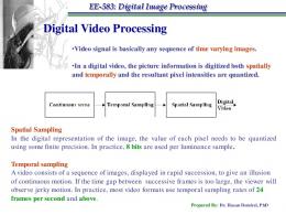
For the full set of operations of this type, please refer to [12]. Note that for all the cases, the DC coefficient remains unchanged because of the fact that each pixel maintains its gray level while its location within the block is changed. These flip-flop and special angle rotation methods are very useful in applications such as image orientation manipulation that is used often in copy machines, printers and scanners. 4.2 MOTION VECTOR PROCESSING (MV RESAMPLING) From a video coding perspective, motion vectors are estimated through block matching in a reference frame. This process is often compute intensive. The key of compressed-domain manipulation of motion vectors is to derive new motion vectors out of existing motion vector information contained in the input compressed bitstream. Consider a motion vector processing scenario that arises in a spatial resolution reduction transcoder. Given the motion vectors for a group of four 16x16 macroblocks of the original video (NxM), how does one estimate the motion vectors for the 16x16 macroblocks in the downscaled video (e.g., N/2xM/2)? Consider forward-predicted macroblocks in a forward-predicted (P) frame, wherein each macroblock is associated with a motion vector and four 8x8 DCT blocks that represent the motion-compensated prediction residual information. The downscale-by-two operation requires four input macroblocks to form a single new output macroblock. In this case, it is necessary to estimate a single motion vector for the new macroblock from the motion vectors associated with the four input macroblocks. The question asked above can be viewed as a motion vector resampling problem. Specifically, given a set of motion vectors MV in the input compressed bitstream, how does one compute the motion vectors MV* of the output compressed bitstream? Motion vector resampling algorithms can be classified into 5 classes as shown in Figure 2 [5]. The most accurate, but least efficient algorithm is Class V, in which one decompresses the original frames into their full pixel representation; and then one performs full search motion estimation on the decompressed frames. Since motion estimation is by far the most compute-intensive part of the transcoding operation, this is a very expensive solution. Simpler motion vector resampling algorithms are

11

Compressed-Domain Video Processing

given in classes I through IV in order of increasing computational complexity, where increased complexity typically results in more accurate motion vectors. Class I MV resampling algorithms calculate each output motion vector based on its corresponding input motion vector. Class II algorithms calculate each output motion vector based on a neighbourhood of input motion vectors. Class III algorithms also use a neighbourhood of input motion vectors, but also consider other parameters from the input bitstream such as quantization parameters and coding modes when processing them. Class IV algorithms use a neighbourhood of motion vectors and other input bitstream parameters, but also use the decompressed frames. For example, the input motion vectors may be used to narrow the search range used when estimating the output motion vectors. Finally, Class V corresponds to full search motion estimation on the decompressed frames. Class I: Process corresponding MV.

Class IV: Partial search ME using coded data.

Class II: Process local neighborhood of MVs. MV

MV buffer

Process

MV*

Class III: Adapt processing based on coded data. MV Data

MV buffer Data buffer

Adaptive Process

MV*

MV

MV buffer

Data

Data buffer

Frame A

Frame Buffer

Frame B

Frame Buffer

Partial Search

MV*

Class V: Full search motion estimation.

Figure 2. Classes of motion vector resampling methods. The conventional spatial-domain approach of estimating the motion vectors for the downscaled video is to first decompress the video, downscale the video in the spatial domain then use one of the several widely known spatialdomain motion-estimation techniques (e.g., [13]) to recompute the motion vectors. This is computationally intensive. A class II approach might be to simply take the average of the four motion vectors associated with the four macroblocks and divide it by two so that the resulting motion vector can be associated with the 16x16 macroblock of the downscaled-by-two video. While this operation requires little processing, the motion vectors obtained in this manner are not optimal in most cases. Adaptive motion vector resampling (AMVR) is a class III approach proposed in [4] to estimate the output motion vectors using the original motion information from the MPEG or H.26x bitstream of the original NxN video sequence. This method uses the DCT blocks to derive the block-activity information for the motion-vector estimation. When comparing the compressed-domain AMVR method to the conventional spatial-domain method, the results suggest that AMVR generates, with significantly less computation, motion vectors for the N/2xM/2 downscaled video that are very close to the optimal motion vector field that would be derived from an N/2xM/2 version of the original video sequence. This weighted average motion vector scheme can also be extended to motion vector downsampling by arbitrary factors. In this operation, the number of participating macroblocks is not an integer. Therefore, the portion of the area

12

Chapter 1

of the participating macroblock is used to weight the contributions of the existing motion vectors. A class IV method for performing motion vector estimation out of existing motion vectors can be found in [14]. In frame rate reduction transcoding, if a P-picture is to be dropped, the motion vectors of macroblocks on the next Ppicture should be adjusted since the reference frame is now different. Youn et al. [14] proposed a motion vector composition method to compute a motion vector from the incoming motion vectors. In this method, the derived motion vector can be refined by performing partial search motion estimation within a narrow search range. The MV resampling problem for the compressed-domain reverse play operation was examined in [5]. In this application, the goal was to compute the “backward” motion vectors between two frames of a sequence when given the “forward” motion vectors between two frames. Perhaps contrary to intuition, the resulting forward and backwards motion vector fields are not simply inverted versions of one another because of the block-based motioncompensated processing used in typical compression algorithms. A variety of MV resampling algorithms is presented in [5], and experimental results are given that illustrate the tradeoffs in complexity and performance. 4.3 MC+DCT PROCESSING The previous section introduced methodologies for deriving output motion vectors from existing input motion vectors in the compressed domain. However, if the newly derived motion vectors are used in conjunction with the original residual data, the result is imperfect and will result in a drift error. To avoid drift error, it is important to reconstruct the original reference frame and re-compute the residual data. This renders the IDCT process as the next computation bottleneck since the residual data is in the DCT domain. Alternatively, DCT domain motion compensation methods, such as the one introduced in [8], can be employed where the reference frames are converted to a DCT representation so that no IDCT is needed. Inverse motion compensation is the process of extracting a 16x16 block given a motion vector in the reference frame. It can be characterised by a group matrix multiplications. Due to the distributive property of the DCT, this operation can be achieved by matrix multiplications of DCT blocks. Mathematically, consider a block g of size 8x8 in a reference frame pointed by a motion vector (x,y). Block g may lie in an area covered by a 2x2 array of blocks (f 1, f 2, f 3, f 4) in the reference frame. g can then be calculated as: 4

g = ∑ m xi f i m yi , where 0 ≤ x, y ≤ 7 . i =1

The shifting matrices mxi and myi are defined as:

  0 0  0 I x  1 , 2 = i   i = 1,3    0 0    I y 0 , and m yi =  , m xi =  0 0 I 8− x  i = 3,4  0 i = 2,4 0 0   I 8− y 0 

Compressed-Domain Video Processing

13

where Iz are identity matrices of size 8x8. In the DCT domain, this operation can be expressed as: 4

G = ∑ M xi Fi M yi ,

(1)

i =1

where Mxi and Myi are the DCT representations of mxi and myi respectively. Since these shifting matrices are constant, they can be pre-computed and stored in the memory. However, the computing of Eq (1) may still be CPUintensive since the shifting matrices may not be sparse enough. To this end, various authors have proposed different methods to combat this problem. Merhav and Bhaskaran [15] proposed to decompose the DCT domain shifting matrices. Matrix decomposition methods are based on the sparseness of the factorized DCT transform matrices. Factorization of DCT transform matrix is introduced in a fast DCT algorithm [16]. The goal of the decomposition is to replace the matrix multiplication with a product of diagonal matrices, simple permutation matrices and more sparse matrices. The multiplication with a diagonal matrix can be absorbed in the quantization process. The multiplication with a permutation matrix can be performed by coefficient permutation. And finally, the multiplication with a sparse matrix requires fewer multiplications. Effectively, the matrix multiplication is achieved with less computation. In an alternative approach, the coefficients in the shifting matrix can be approximated so that floating point multiplication can be replaced by integer shift and add operation. Work of this kind is introduced in [17]. Effectively, fewer basic CPU operations are needed since multiplication operations are avoided. A similar method is also used in [18] for DCT domain downsampling of images by employing the approximated downsampling matrices. To further reduce the computation complexity of the DCT domain motion compensation process, a look-up-table (LUT) based method [19] is proposed by modelling the statistical distribution of DCT coefficients in compressed images and video sequences and precomputing all possible combinations of M xi Fi M yi as in Eq (1). As a result, the matrix multiplications are reduced to simple table look-ups. Using around 800KB of memory, the LUT-based method can save more than 50% of computing time. 4.4 RATE CONTROL/BUFFER REQUIREMENTS Rate control is another important issue in video coding. For compressed domain processing, the output of the process should also be confined to a certain bitrate so that it can be delivered in a constant transmission rate. Eleftheriadis and Anastassiou [20] have considered rate reduction by an optimal truncation or selection of DCT coefficients. Since fewer coefficients are coded, a lower number of bits are spent in coding them. Nakajima et al [21] achieve the similar rate reduction by re-quantization using a larger quantization step size. For compressed domain processing, it is important for the rate control module to use compressed domain information existing in the original stream. This is a challenging problem, since the compressed bitstream lacks information that was available to the original encoder. To illustrate this

14

Chapter 1

problem, consider TM5 rate control, which is used in many video coding standards. This rate controller begins by estimating the number of bits available to code the picture, and computes a reference value of the quantization parameter based on the buffer fullness and target bitrate. It then adaptly raises or lowers the quantization parameter for each macroblock based on the spatial activity of that macroblock. The spatial activity measure as defined in TM5 as the variance of each block:

V=

1 64 1 64 2 ∑ (Pi − Pmean ) , where Pmean = ∑ Pi . 64 i =1 64 i =1

However, the pixel domain information Pi may not be available in the compressed domain processing. In this case, the activity measure has to be derived from the DCT coefficients instead of the pixel domain frames. For example, the energy of quantized AC coefficients in the DCT block can be used as a measure of the variance. It has been shown in [4] that this approach achieves satisfactory rate control. In addition, the target bit budget for a particular frame can be derived from the bitrate reduction factor and the number of bits spent for the corresponding original frame, which is directly available from the original video stream. 4.5 FRAME CONVERSIONS Frame conversions are another basic tool that can be used in compresseddomain video processing operations [22]. They are especially useful in frame-level processing applications such as splicing and reverse play. Frame conversions are used to convert coded frames from one prediction mode to another to change the prediction dependencies in coded video streams. For example, an original video stream coded with I, P, and B frames may be temporarily converted to a stream coded with all I frames, i.e. a stream without temporal prediction, to facilitate pixel-level editing operations. Also, an IPB sequence may be converted to an IB sequence in which P frames are converted to I frames to facilitate random access into the stream. Also, when splicing two video sequences together, frame conversions can be used to remove prediction dependencies from video frames that are not included in the final spliced sequence. Furthermore, one may wish to use frame conversions to add prediction dependencies to a stream, for example to convert from an all I-frame compressed video stream to an I and P frame compressed stream to achieve a higher compression rate. A number of frame conversion examples are shown in Figure 3. The original IPB sequence is shown in the top. Examples of frame conversions that remove temporal dependencies between frames are given: specifically P-to-I frame, B-to-Bfor conversion, and B-to-Bback conversion. These operations are useful for editing operations such as splicing. Finally, an example of I-to-P conversion is shown in which prediction dependencies are added between frames. This is useful in applications that require further compression of a pre-compressed video stream. Frame conversions require macroblock-level and block-level processing because they modify the motion vector and DCT coefficients of the compressed stream. Specifically, frame conversions require examining each macroblock of the compressed frame, and when necessary changing its coding mode to an appropriate dependency. Depending on the conversion, some, but not all, macroblocks may need to be processed. An example in

15

Compressed-Domain Video Processing

which a macroblock may not need to be processed is in a P-to-I frame conversion. Since P frames contain i- and p- type macroblocks and I frames contain only i-type macroblocks; a P-to-I conversion requires converting all p-type input macroblocks to i-type output macroblocks; however, note that itype input macroblocks do not need to be converted. The list of frame types and allowed macroblock coding modes are shown in the upper right table in Figure 3. The lower right table shows macroblock conversions needed for some frame conversion operations. These conversions will be used in the splicing and reverse play applications described in Section 5. The conversion of a macroblock from p-type to i-type can be performed with the inverse motion compensation process introduced in Subsection 4.3.

Original

P B B

I

B B P

P to I

P B B

I

B B

I

B to Bfor

P Bf Bf I Bf Bf P

B to Bback

P Bb Bb I Bb Bb P

Frame Type

MB Type

I P B Bintra Bforw Bback

i i, p i, bforw, bback, b i i, bforw i, bback

Frame Conversion

MB Conversion

P→I

p→i b → bforw bback → i b → bback bforw → i b→i bback → i bforw → i

B → Bforw

I to P

P B B P B B P

B → Bback B → Bintra

Figure 3. Frame conversions and required macroblock conversions. One should note that in standards like MPEG, frame conversions performed on one frame may affect the prediction used in other frames because of the prediction rules specified by I, P, and B frames. Specifically, I-to-P and P-to-I frame conversions do not affect other coded frames. However, I-to-B, B-to-I, P-to-B, and B-to-P frame conversions do affect other coded frames. This can be understood by considering the prediction dependency rules of MPEG. Specifically, since P frames are specified to depend on the nearest preceding I or P frame and B frames are specified to depend on the nearest surrounding I or P frames, it is understandable that frame conversions of certain types will affect the prediction dependency tree inferred from the frame coding types.

5. APPLICATIONS This section shows how the compressed domain processing methods described in Section 4 can be applied to video transcoding and video processing/editing applications. Algorithms and architectures are described for a number of CDP operations.

16

Chapter 1

5.1 COMPRESSED-DOMAIN TRANSCODING APPLICATIONS With the introduction of the next generation wireless networks, mobile devices will access an increasing amount of media-rich content. However, a mobile device may not have enough display space to render content that was originally created for desktop clients. Moreover, wireless networks typically support lower bandwidths than wired networks, and may not be able to carry media content made for higher-bandwidth wired networks. In these cases, transcoders can be used to transform multimedia content to an appropriate video format and bandwidth for wireless mobile streaming media systems. A conceptually simple and straightforward method to perform this transcoding is to decode the original video stream, downsample the decoded frames to a smaller size, and re-encode the downsampled frames at a lower bitrate. However, a typical CCIR601 MPEG-2 video requires almost all the cycles of a 300Mhz CPU to perform real-time decoding. Encoding is significantly more complex and usually cannot be accomplished in real time without the help of dedicated hardware or a high-end PC. These factors render the conceptually simple and straightforward transcoding method impractical. Furthermore, this simple approach can lead to significant loss in video quality. In addition, if transcoding is provided as a network service in the path between the content provider and content consumer, it is highly desirable for the transcoding unit to handle as many concurrent sessions as possible. This scalability is critical to enable wireless networks to handle user requests that may be very intense at high load times. Therefore, it is very important to develop fast algorithms to reduce the compute and memory loads for transcoding sessions. 5.1.1 Compressed-Domain Transcoding Architectures Video processing applications often involve a combination of spatial and temporal processing. For example, one may wish to downscale the spatial resolution and lower the frame rate of a video sequence. When these video processing applications are performed on compressed video streams, a number of additional requirements may arise. For example, in addition to performing the specified video processing task, the output compressed video stream may need to satisfy additional requirements such as maximum bitrate, buffer size, or particular compression format (e.g. MPEG-4 or H.263). While conventional approaches to applying traditional video processing operations on compressed video streams generally have high compute and memory requirements, the algorithmic optimizations described in Section 4 can be used to design efficient compressed-domain transcoding algorithms with significantly reduced compute and memory requirements. A number of transcoding architectures were discussed in [23][24][25][26]. Figure 4 shows a progression of architectures that reduce the compute and memory requirements of such applications. These architectures are discussed in the context of lowering the spatial and temporal resolution of the video from S0,T0 to S1,T1 and lowering the bitrate of the bitstream from R0 to R1. The top diagram shows the conventional approach to processing the compressed video stream. First the input compressed bitstream with bitrate R0 is decoded into its decompressed video frames, which have a spatial resolution and temporal frame rate of S0 and T0. These frames are then processed temporally to a lower frame rate T1 < T0 by dropping appropriate

17

Compressed-Domain Video Processing

frames. The spatial resolution is then reduced to S1 < S0 by spatially downsampling the remaining frames. The resulting frames with resolution S1,T1 are then re-encoded into a compressed bitstream with a final bitrate of R1