Compressed Indexes for Dynamic Text Collections - CiteSeerX

Compressed Indexes for Dynamic Text Collections HO-LEUNG CHAN University of Hong Kong and WING-KAI HON National Tsing Hua University and TAK-WAH LAM University of Hong Kong and KUNIHIKO SADAKANE Kyushu University Let T be a string with n characters over an alphabet of constant size. The recent breakthrough on compressed indexing allows us to build an index for T in optimal space (i.e., O(n) bits), while supporting very efficient pattern matching [Ferragina and Manzini 2000; Grossi and Vitter 2000]. Yet the compressed nature of such indexes also makes them difficult to update dynamically. This paper extends the work on optimal-space indexing to a dynamic collection of texts. Our first result is a compressed solution to the library management problem, where we show an index of O(n) bits for a text collection L of total length n, which can be updated in O(|T | log n) time when a text T is inserted or deleted from L; also, the index supports searching the occurrences of any pattern P in all texts in L in O(|P | log n + occ log2 n) time, where occ is the number of occurrences. Our second result is a compressed solution to the dictionary matching problem, where we show an index of O(d) bits for a pattern collection D of total length d, which can be updated in O(|P | log2 d) time when a pattern P is inserted or deleted from supports ¡ D; also, the index ¢ searching the occurrences of all patterns of D in any text T in O (|T | + occ) log2 d time. When compared with the O(d log d)-bit suffix tree based solution of Amir et al. [1995], the compact solution increases the query time by roughly a factor of log d only. The solution of the dictionary matching problem is based on a new compressed representation of a suffix tree. Precisely, we give an O(n)-bit representation of a suffix tree for a dynamic collection of texts whose total length is n, which supports insertion and deletion of a text T in O(|T | log2 n) time, as well as all suffix tree traversal operations, including forward and backward suffix links. This work can be regarded as a generalization of the compressed representation of static texts. In the study of the above result, we also derive the first O(n)-bit representation for maintaining n pairs of balanced parentheses in O(log n/ log log n) time per operation, matching the time complexity of the previous O(n log n)-bit solution. This paper combines the results of two papers which appeared in Proceedings of Symposium on Combinatorial Pattern Matching (CPM), 2004, and in Proceedings of Symposium on Discrete Algorithms (SODA), 2005, respectively. Authors’ contacts: H. Chan ([email protected]), W. Hon ([email protected]), T. Lam ([email protected]), and K. Sadakane ([email protected]). Permission to make digital/hard copy of all or part of this material without fee for personal or classroom use provided that the copies are not made or distributed for profit or commercial advantage, the ACM copyright/server notice, the title of the publication, and its date appear, and notice is given that copying is by permission of the ACM, Inc. To copy otherwise, to republish, to post on servers, or to redistribute to lists requires prior specific permission and/or a fee. c 20YY ACM 0000-0000/20YY/0000-0001 $5.00 ° ACM Journal Name, Vol. V, No. N, Month 20YY, Pages 1–30.

2

·

Ho-Leung Chan et al.

Categories and Subject Descriptors: E.1 [Data Structures]: ; E.4 [Coding and Information Theory]: Data Compaction and Compression; F.2.2 [Non-numerical Algorithms and Problems]: Pattern Matching; H.3.1 [Content Analysis and Indexing]: Dictionaries; Indexing Methods General Terms: Algorithms, Design, Theory Additional Key Words and Phrases: Compressed Suffix Tree, String Matching

1. INTRODUCTION Indexing a text to support efficient pattern matching has been studied extensively. The recent breakthrough allows us to build an index in optimal space (i.e., O(n) bits for a text with n characters over a constant-size alphabet), without sacrificing the speed of pattern matching. This paper extends the work of optimal-space indexing to a dynamic setting. In particular, we consider two well-studied problems, known as the library management problem and the dictionary matching problem. An introduction to these two problems are described below. Afterwards, we discuss a basic data structure problem for maintaining a sequence of balanced parentheses, which serves as a tool for the solution of our dictionary matching problem. 1.1 Library Management The library management problem [McCreight 1976] is defined as follows: We need to maintain a collection L of texts of total length n; from time to time, a text may be inserted or deleted from L (thus changing the total length), and a pattern P may be given and its occurrences in L are to be reported. This problem occurs naturally in the management of homepages (e.g., Google), DNA/protein sequences [Mewes and Heumann 1995], and many other real-life applications. For the static case where the texts in L never change, we can concatenate all the texts into one and then build a suffix tree [McCreight 1976; Weiner 1973] or a suffix array [Manber and Myers 1993] for the concatenated text; the searching time for a pattern P with length p is O(p+occ) and O(p+log n+occ), respectively, where occ is the number of occurrences of P in L. Note that a suffix tree of a string is a compact trie containing all suffixes of the string, while a suffix array is an array of all suffixes of the string arranged in lexicographical order. Both indexes occupy O(n log n) bits of storage. For indexing a huge amount of web pages or DNA/protein sequences, this space requirement may be too demanding. For example, the suffix tree for the human genome (totally 3G characters) takes 40G bytes of memory, while the suffix array takes 13G bytes [Kurtz 1999]. Recently, two exciting results have been made on providing indexes occupying only O(n) bits, yet supporting efficient pattern searching. Essentially, both of them can be considered as another form of the suffix array, storing in a compact manner. The first one is the compressed suffix arrays (CSA) [Grossi and Vitter 2000; 2005], which supports pattern searching in O(p log n + occ log² n) time, for any fixed ² > 0. The second one is the FM-index [Ferragina and Manzini 2000; 2005], with which pattern searching can be done in O(p + occ log² n) time.1 These data structures are 1 There

are other variants of the CSA [Grossi et al. 2003; 2004] and FM-index [Ferragina et al.

ACM Journal Name, Vol. V, No. N, Month 20YY.

Compressed Indexes for Dynamic Text Collections

·

3

also sound in practice. Using CSA or FM-index, one can index the human genome with 1.5G bytes of memory [Hon et al. 2004]. For the dynamic case where texts can be inserted into or deleted from L, if O(n log n) bits of space is allowed, one can build a generalized suffix tree (i.e., a single compact trie containing the suffixes of each text in L). Then, to insert or delete a text of length t in L, we update the generalized suffix tree by adding or removing all suffixes of the text, which can be done in O(t) time. For searching a pattern P , the time remains O(p + occ). To reduce space, one may attempt to ‘dynamize’ a compressed index such as CSA or FM-index. Indeed, Ferragina and Manzini [2000] have demonstrated how to maintain multiple FM-indexes so as to support a dynamic collection of texts. Their solution requires O(n + m log n) bits, where m is the number of texts in the collection. Pattern matching is slowed down slightly, using O(p log3 n + occ log n) time. But insertion and deletion has only an amortized performance guarantee; precisely, insertion and deletion of a text of length t take O(t log n) and O(t log2 n) amortized time, respectively. In the worst case, a single insertion or deletion may require re-constructing many of the FM-indexes, using Θ(n/ log2 n) time even if t is very small. In this paper, we introduce a compressed index for the dynamic library management problem, whose performance is stated in the following theorem. Theorem 1.1. Let L = {T1 , T2 , · · · , Tm } be a set of m distinct strings over a constant-size alphabet Σ. Let n be the total length of all strings in L. We can maintain L in O(n)-bit space such that inserting or deleting a text T of length t in L takes O(t log n) time and searching for a pattern P of length p takes O(p log n + occ log2 n) time, where occ is the number of occurrences. Note that the time complexities of all operations are measured in the worst case (instead of the amortized case). To our knowledge, this is the first result that requires only O(n) bits, yet supporting both update and searching efficiently, i.e., in O(t logO(1) n) and O((p + occ) logO(1) n) time, respectively. Our techniques. Technically speaking, our compressed index is based on CSA and FM-index. Yet a few more techniques are needed to achieve the optimal space requirement and efficient updating. Firstly, recall that the index proposed by Ferragina and Manzini [2000] for the library management problem requires O(n + m log n) bits. We have a simple but useful trick in organizing the texts, which eliminates the m log n term, thus avoiding the use of a lot of space when the collection involves a lot of very short strings. Secondly, the original representations of CSA and FM-index do not support updates efficiently. For instance, the index proposed by Ferragina and Manzini [2000] essentially requires re-building one or more FM-index whenever a text is inserted. Inspired by a dynamic representation of CSA in [Lam et al. 2002], we manage to dynamize the CSA and the FM-index to support efficient updates to a collection of texts. With either of them, we can immediately obtain an O(n)-bit index that supports updates in O(t log2 n) time. For 2004; M¨ akinen and Navarro 2004], which achieve space bounds in terms of the entropy of the text. The space can be o(n) bits for low entropy texts. However, in this paper, we will stick to the original definitions of CSA and FM-index. ACM Journal Name, Vol. V, No. N, Month 20YY.

4

·


pattern matching, using FM-index alone can achieve O(p log n + occ log2 n) time, and using CSA alone takes O(p log2 n + occ log2 n) time. Last but not the least, we find that FM-index and CSA can complement each other nicely to further improve the update time. Roughly speaking, in the process of updating such suffix-array based compressed indexes, there are two pieces of crucial information needed. We observe that one of them can be provided quickly by FM-index, and the other can be provided quickly by CSA. Thus, by maintaining both CSA and FM-index together, we can perform the update more easily, so that the update time can be improved to O(t log n). 1.2 Dictionary Matching and Compressed Suffix Trees The dictionary matching problem is a dual problem to library management, which is defined as follows: We need to maintain a collection D of patterns of total length d; from time to time, a pattern may be inserted or deleted from D (thus changing the total length), and a text T may be given such that the occurrences of all patterns of D in T are to be reported. This problem is well-studied in the literature [Aho and Corasick 1975; Amir and Farach 1991; Amir et al. 1992; Amir et al. 1994; Amir et al. 1995; Sahinalp and Vishkin 1996], and an important example application is the management of a gene bank. The dictionary matching problem can readily be solved using O(d log d) bits based on suffix trees, even in the dynamic case which allows insertion or deletion of patterns in D. In particular, Amir et al. [1995] showed that insertion or deletion of a pattern P of length p can be done in O(p log d/ log log d) time and a dictionary matching query for a text T of length t takes O((t + occ) log d/ log log d) time.2 To solve the dictionary matching problem with a compressed index, it is natural to ask whether we can have a compressed version of a suffix tree for a dynamic collection of texts. That is, we want to support queries about the suffix tree structure (namely, parent, child, sibling, edge label, and leaf label) and suffix links, while allowing efficient update due to insertion and deletion of texts. Sadakane [2007] has made a step towards this goal; his work gives an O(n)-bit representation for a suffix tree which can avoid storing pointers, but his work assumes a static text (or a static collection of texts); the underlying data structures are rigidly packed and cannot be updated efficiently. Our results. In this paper, we devise a compressed implementation of a suffix tree for a dynamic collection of texts, based on which and adapting the work of Amir et al. [1995], we are able to solve the dynamic dictionary matching problem as stated in the following theorem. Theorem 1.2. Let D = {P1 , P2 , . . . , Pm } be a set of m distinct patterns over a constant-size alphabet Σ. Let d be the total length of all patterns in D. We can maintain D in O(d)-bit space such that inserting or deleting a pattern P of length p ¡takes O(p log2 d)¢ time. A dictionary matching query for a text T of length t takes O (t + occ) log2 d time, where occ is the number of occurrences. Our techniques. As mentioned, we want to extend the compressed suffix tree 2 Sahinalp

and Vishkin [Sahinalp and Vishkin 1996] devised a non-suffix-tree-based data structure called fat-tree, and improved the update time to O(p), and query time to O(t + occ). ACM Journal Name, Vol. V, No. N, Month 20YY.


·

5

of Sadakane [2007] to support dynamic updates. The challenge lies in two aspects: structural and algorithmic. Structurally, our compressed suffix tree should not only be compact, but also be flexible enough to allow efficient updates. Algorithmically, we have to find efficient updating methods that are tailored for the underlying data structures. This often requires supporting operations other than the basic navigational operations for traversing the suffix tree. In this paper, we give the first O(n)-bit representation of a suffix tree that allows efficient updates. Our solution is comprised of several dynamic data structures for representing CSA and FM-index, as well as the tree structure. With our solution, retrieving an edge label and leaf label requires O(log2 n) time, while other navigation queries, including suffix links, can be performed in O(log n) time. More importantly, we allow the retrieval of backward suffix links [Weiner 1973], which turns out to be crucial for supporting efficient updates of the representation. Apparently, representing backward suffix links is more demanding than that for the (forward) suffix links, because each internal node of a suffix tree may have more than one backward suffix link, while some internal nodes may have none. Nevertheless, we are able to show that FM-index already allows us to recover the backward suffix links efficiently. If we maintain a suffix tree to represent a collection of texts, we can use McCreight’s method [McCreight 1976] to insert or delete a text X efficiently. In McCreight’s insertion method, the suffix tree is updated by adding suffixes of X one by one from the longest to the shortest one. If we try to extend this idea of insertion to maintain our compressed suffix tree, this will create a fundamental technical problem as both CSA and FM-index should be constructed and updated by adding suffixes from the shortest to the longest, since CSA and FM-index are only well-defined for representing a collection of texts and all their suffixes. This motivates us to take an asymmetric approach to update our compressed suffix tree with the provision of the two types of suffix links. Precisely, insertion is based on the framework of Weiner’s suffix tree construction method [Weiner 1973], where we start from adding the shortest suffix to the longest one, exploiting backward suffix links. For deletion, it is based on McCreight’s method with forward suffix links. Both can be done in O(|X| log2 n) time. Another interesting point is that edge labels are only implicitly stored by the compact data structures, which can be computed efficiently when needed. Furthermore, when the data structures are updated, the correctness of the edge labels are automatically maintained. 1.3 Parentheses Maintenance To represent a suffix tree, we need a compact representation of the tree structure. This can be done using a sequence of balanced parentheses [Jacobson 1989; Munro and Raman 2001]. For a sequence of n pairs of balanced parentheses, the basic queries include find match and enclose, which find the position of the matching parenthesis and the position of the nearest pair of enclosing parentheses, respectively. For the static case, the best known solution is by Munro and Raman [2001], which supports these operations in constant time and occupies only 2n + o(n) bits. When we need to maintain the parentheses under insertion and deletion, the best result is by Amir et al. [1995], which requires O(n log n) bits, while supporting each operation, including an update, in O(log n/ log log n) time. In this paper, we ACM Journal Name, Vol. V, No. N, Month 20YY.

6

·


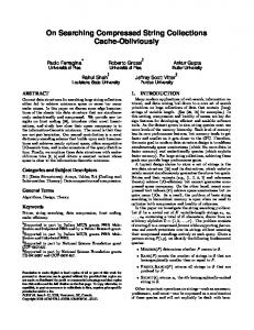
propose the first O(n)-bit representation for maintaining the balanced parentheses, with O(log n/ log log n) time per operation, thus matching the performance of the best dynamic result with reduced space requirement. As for theoretical interest, we observe that the classical problem for maintaining a subset of items in [1, n] under updates, with rank and select queries supported,3 can be reduced to the parentheses maintenance problem. Then based on the lower bound result of Fredman and Saks [1989], we can conclude that for any data structure for the parentheses maintenance problem, there exists a sequence of operations requiring Ω(log n/ log log n) amortized time per operation. Finally, we also consider a more complicated operation called double enclose, which finds the nearest parenthesis pair that encloses two input pairs of parentheses. We show that with an O(n)-bit data structure, this operation can be done in O(log n) time. 1.4 Organization The remaining of the paper is organized as follows. Section 2 gives a brief review on the suffix trees, suffix arrays, CSA and FM-index. Sections 3 is devoted to our solution for the library management problem. In Section 4, we describe the compressed suffix tree, and show how it can be used to solve the dictionary matching problem. The data structure for parentheses maintenance is shown in Section 5. We conclude the paper in Section 6. 2. PRELIMINARIES In this section, we give a brief review on suffix trees [McCreight 1976; Weiner 1973], suffix arrays [Manber and Myers 1993], Compressed Suffix Arrays [Grossi and Vitter 2000], and FM-index [Ferragina and Manzini 2000]. Let T [1, n] = T [1]T [2] · · · T [n] be a string of length n over a finite alphabet Σ. For any i = 1, . . . , n, T [i, n] is a suffix of T . Suffix Trees. The suffix tree for a string T is a compact trie that contains all suffixes of T . Each edge represents some substring T [i, j] of T , called the edge label, which is stored as the pair (i, j) for space saving. Each leaf represents some suffix T [i, n] of T , and i is called the leaf label of the leaf. In addition, the suffix tree contains a suffix link for each internal node, which is defined as follows. We define the path label of a node u as the string formed by concatenating the edge labels on the path from the root to u. Then, the suffix link of u is a pointer from u to another node v such that the path label of v is the same as the path label of u with the first character removed. Note that suffix link for every internal node exists and is unique. A suffix tree can be stored in O(n log n) bits. See Figure 1 for an example of the suffix tree for a string T = acaaccg$, where the edge label of an edge is shown explicitly by the substring of T adjacent to the edge, the leaf label of a leaf is shown by the integer contained in the leaf, and the suffix link of an internal node is shown by the dashed arrow pointing outwards from the node. 3 For any given integer i, the rank query returns the number of items in the subset which is at most i; for any given integer j, the select query finds the j-th smallest item in the subset.



Fig. 1.

·

7

Example of a suffix tree

The generalized suffix tree for a text collection is a suffix tree containing the suffixes of all texts in the collection. Each edge is stored by three integers, specifying which substring of which text its edge label comes from. The generalized suffix tree can be updated efficiently to allow insertion or deletion of a text in the collection. Precisely, insertion or deletion of a text of length t can be done in O(t) time. Searching where a pattern P [1, p] appears in the collection is also efficient, which can be done using O(p + occ) time, where occ denotes the number of occurrences. Suffix Arrays, CSA and FM-index. Note that for any internal node in the suffix tree, the edges connecting it to its children will have distinct first characters in their edge labels. We assume that each internal node orders these edges from left to right based on the lexicographical order of the corresponding edge label. Then, if we traverse the leaves of the suffix tree for T from left to right and enumerate the leaf labels along the way, we obtain the suffix array SA[1, n] of T , which is an array of integers such that T [SA[i], n] is the lexicographically i-th smallest suffix of T . A suffix array can be stored in O(n log n) bits. Both the CSA and FM-index are compressed versions of the suffix array, as they are able to retrieve any SA value in O(log n) time, but they require less amount of storage space compared to the original suffix array. For CSA, its main component is the function Ψ[1, n] where Ψ[i] = SA−1 [SA[i] + 1]. In other words, if i is the lexicographical order of the suffix T [SA[i], n], then Ψ[i] gives the lexicographical order of the suffix T [SA[i] + 1, n]. We can count the number of occurrences of a pattern P [1, p] in T using O(p log n) queries to Ψ [Grossi and Vitter 2000]. The CSA can be stored in O(n) bits. For FM-index, its main component is the function count, which is defined based on the BWT array [Burrows and Wheeler 1994]. For i in [1, n], BWT[i] is the characACM Journal Name, Vol. V, No. N, Month 20YY.

8

·


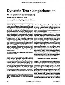
ter T [SA[i] − 1]. For each character c in Σ and i in [1, n], the function count(c, i) computes the number of times the character c appears in BWT[1, i]. We can count the number of occurrences of a pattern P [1, p] in T using O(p) queries to count [Ferragina and Manzini 2000]. Similar to the CSA, FM-index can be stored in O(n) bits. See the figure below for an example of the SA, Ψ, BWT and count functions. T = acaaccg$ i 1 2 3 4 5 6 7 8

suffixes in sorted order $ aaccg$ acaaccg$ accg$ caaccg$ ccg$ cg$ g$

SA[i]

Ψ[i]

BWT[i]

count(“a”, i)

count(“c”, i)

8 3 1 4 2 5 6 7

3 4 5 6 2 7 8 1

g c $ a a a c c

0 0 0 1 2 3 3 3

0 1 1 1 1 1 2 3

The CSA and FM-index are closely related. In the following, we give two lemmas that relate the Ψ function of CSA and the count function of FM-index. Firstly, observe that suffixes beginning with the same character correspond to a consecutive region in SA. For example, in the above figure, SA[2, 4] and SA[5, 7] correspond to suffixes beginning with “a” and “c”, respectively. The above regions can be calculated as follows: For each character c, let α(c) be the number of suffixes beginning with a character less than c, and let #(c) be the number of suffixes that begin with c. Then, [α(c) + 1, α(c) + #(c)] is the region in SA that corresponds to suffixes beginning with c. We will store all #(c) values explicitly, so that #(c) for any c can be retrieved in constant time. Then, α(c) for any c in Σ and T [SA[i]] for any i in [1, n] can be computed in constant time, and we have the following lemmas. Lemma 2.1. For any c in Σ and any i in [1, n], we can compute count(c, i) using O(log n) queries to Ψ. Proof. Observe that T [SA[j]] = c if and only if BWT[Ψ[j]] = c. This implies that count(c, i) is the number of j satisfying T [SA[j]] = c and Ψ[j] ≤ i. However, for T [SA[j]] = c, j must be in the region [α(c) + 1, α(c) + #(c)]. Thus, count(c, i) is equal to the number of j in [α(c) + 1, α(c) + #(c)] satisfying Ψ[j] ≤ i. As shown in [Grossi and Vitter 2000; Sadakane 2000], Ψ[α(c) + 1, α(c) + #(c)] is an increasing sequence for any c. Thus, count(c, i) can be found by a binary search on Ψ[α(c) + 1, α(c) + #(c)], using O(log n) queries to Ψ. Lemma 2.2. For any i in [1, n], we can compute Ψ[i] using O(log n) queries to the count function. Proof. Let c = T [SA[i]] and y = i − α(c). Both c and y can be computed in constant time based on the stored #(c) values. Now, suppose that the following claim is correct: BWT[Ψ[i]] is the y-th c in the BWT array. Then, Ψ[i] is the smallest k such that count(c, k) = y. As count(c, ·) is monotonic increasing, that the value of k (and thus Ψ[i]) can be found based on binary search, using O(log n) queries to the count function. ACM Journal Name, Vol. V, No. N, Month 20YY.


·

9

To prove the claim, we first show that BWT[Ψ[i]] = c. This is true since BWT[Ψ[i]] = T [SA[i]]. Next, we observe that for each j in [1, Ψ[i]] with BWT[j] = c, the suffix cT [SA[j], n] is a distinct suffix of T that begins with c and lexicographically smaller than or equal to T [SA[i], n]. In other words, if r denotes the rank of the suffix T [SA[i], n] among all suffixes of T that begin with c, BWT[Ψ[i]] is the r-th c in BWT. Clearly, r = i − α(c) = y. This completes the proof of the claim, and the lemma follows. To conclude this section, we state a lemma to demonstrate the searching ability provided by the count function. Lemma 2.3 [Ferragina and Manzini 2000]. Let P be any pattern and let c be any character in Σ. Denote the lexicographical order of P among all suffixes of T (i.e., 1 + the number of such suffixes less than P ) as i. Then, count(c, i−1)+α(c)+1 is the lexicographical order of cP among all suffixes of T . We refer to an execution of the above lemma a backward search step. Applying the backward search steps repeatedly, we can find the number of occurrences of any pattern P [1, p] in T , using O(p) queries to the count function. Such a searching method is known as the backward search algorithm in the literature. 3. COMPRESSED INDEX FOR DYNAMIC LIBRARY MANAGEMENT This section is devoted to proving Theorem 1.1, where we show an O(n)-bit index for maintaining a collection L of texts of total length n, with characters drawn from a constant-size alphabet Σ; the index supports inserting or deleting a text of length t in O(t log n) time, and searching for a pattern P [1, p] in O(p log n + occ log2 n) time. Our compressed index consists of three data structures, namely, COUNT , MARK , and PSI , that correspond to the dynamic representations of the count functions of FM-index, the auxiliary data structure to retrieve SA values, and the Ψ function of CSA, respectively. We first introduce COUNT , which is the core data structure that already supports counting the occurrences of a pattern P in L efficiently, and fast insertion or deletion of texts. Afterwards, we discuss how to exploit MARK and PSI to support efficient enumeration of the positions where a pattern P occurs, and further speed up the updating process. Consider a set of texts L = {T1 , T2 , . . . , Tm } over a constant-size alphabet Σ. We assume that the texts are distinct, and each text T starts with a special character $ in Σ, where $ is alphabetically smaller than all other characters in Σ and it does not appear in any other part of a text. Denote the total length of all texts as n. In case the contents of the text collection is changed, we always label the existing texts in L in such a way that Tj refers to the lexicographically rank-j text currently in L. Conceptually, we want to construct a suffix array SA for the texts by listing out all suffixes of all texts in lexicographical order. For i in [1, n], SA[i] = (j, k) if the suffix Tj [k, |Tj |] is the rank-i suffix among all suffixes of all texts. To insert a text T to L, we insert all suffixes of T into the SA. Similarly, to delete a text ACM Journal Name, Vol. V, No. N, Month 20YY.

10

·


from L, we delete all suffixes of T from SA. Searching for a pattern P is done by determining the interval [x, y] such that each suffix corresponding to SA[x] up to SA[y] has P as a prefix. In other words, SA[x], SA[x + 1], . . . , SA[y] are the starting positions of all locations where P occurs in L. 3.1 The COUNT Data Structure Due to the space restriction, we cannot directly store the SA table. Instead, we use the FM-index, which requires only O(n) bits, to represent the SA table implicitly. The FM-index for L consists of the function count(c, i) for each c in Σ, which returns the number of occurrences of character c in BWT[1, i], where BWT[i] is defined as the character Tj [k − 1] if SA[i] = (j, k).4 Note that this definition is analogous to the original definition of FM-index for a single text, so that we refer the above BWT array as the Burrows-Wheeler transformation of L. We implement the count(c, i) function with a dynamic data structure COUNT , whose performance is summarized in the lemma below. Lemma 3.1. We can maintain the COUNT data structure using O(n) bits space such that each of the following operations is supported in O(log n) time. —Report(c, i): Returns the value of count(c, i). —Insert(c, i): Updates all count functions due to a character c inserted to the position i of BWT. —Delete(i): Updates all count functions due to a character deleted from the position i of BWT. Proof. To implement COUNT , we store |Σ| lists of bits, denoted as COUNTc for each c in Σ. Each list is n-bit long, with COUNTc [i] = 1 if BWT[i] = c and COUNTc [i] = 0 otherwise. To support updates easily, for each list COUNTc , we partition it into segments of log n bits to 2 log n bits. The segments are stored in the nodes in a red-black tree, so that a left to right traversal of the tree gives the list COUNTc . Precisely, each node u in the tree contains the following fields. —A color bit (red or black), a pointer to parent, a pointer to the left child and a pointer to the right child. —A segment of bits, with length log n to 2 log n. —An integer size indicating the total number of bits contained in the subtree rooted at u. —An integer sum indicating the total number of 1’s contained in the subtree rooted at u. To support the function count(c, i), we use the size value in each node to traverse the tree of COUNTc and locate the node u that contains the bit COUNTc [i]. We record the number of 1’s in the segment of u up to this bit,5 and also the sum in the left child of u. Then, we traverse from u to the root. For every left parent v on the path, we record the number of 1’s in the segment of v and also the sum in 4 Precisely, 5 This

the index k − 1 in Tj [k − 1] is defined under modulo-|Tj | arithmetic. can be done in constant time in RAM with a universal decoding table of o(n) bits [Jacobson

1989]. ACM Journal Name, Vol. V, No. N, Month 20YY.


·

11

the left child of v. Summing up all these recorded values, we obtain the number of 1’s in the list of COUNTc up to the bit COUNTc [i], which equals count(c, i). The whole process takes O(log n) time. To update the COUNT data structure when a character c is inserted to position i of BWT, we insert a bit 1 to position i of COUNTc and insert a bit 0 to position i of COUNTc 0 for each c0 6= c. The time required is O(log n). Deletion of a character from BWT can be done in the opposite way in O(log n) time. For the space requirement, we note that each node takes O(log n) bits and there are O(n/ log n) nodes. Thus, the space requirement is O(n) bits. This completes the proof of the lemma. Note that COUNT allows efficient update which is needed when the BWT array is changed due to insertion or deletion of texts. Our implementation is different from the original one in [Ferragina and Manzini 2000], where the count functions are stored in a data structure which is difficult to update (but allows constant-time query). Pattern matching. Similar to the case of a single text, we define #(c) for each character c to be the number of suffixes whose first character is c, and maintain these values explicitly to allow constant-time retrieval. Then, α(c) or T [SA[i]] can be computed in constant time. Together with the COUNT data structure, we can support counting the occurrences of P [1, p] in L in O(p log n) time, using the backward search algorithm as follows: Firstly, the rank of P [p] among all suffixes can be computed in constant time by 1 + α(P [p]). Then, by Lemma 2.3, we can find the rank of P [p − 1, p] using one query to the count functions. The process is repeated, so that eventually we can find the rank (say, x) of P [1, p]. Similarly, we can find the rank (say, y) of P [1, p]z, where z is assumed to be an arbitrary string of rank n + 1 among all suffixes. Then, the number of occurrences of P is y − x. As the whole process requires O(p) queries to the count functions and each query takes O(log n) time, the total time follows. Text insertion. To insert a text T [1, t], we conceptually insert all suffixes of T to SA, starting from the shortest one. The rank of T [t] among the suffixes stored in SA, denoted as i, is 1 + α(T [t]). Conceptually, we want to insert T [t] to the i-th entry in SA. However, as the SA table is not stored explicitly, we reflect the change in SA by the corresponding change in BWT instead, where we insert the character T [t − 1] to the i-th position of the BWT array. This is done by performing Insert(T [t − 1], i) provided by COUNT . Next, to insert (conceptually) the suffix T [t−1, t] to SA, let i0 be the rank of T [t−1, t] among the suffixes stored in the updated SA, which is found by one backward search step in the updated COUNT data structure. The required change in SA is reflected by inserting T [t − 2] to the i0 -th position of BWT. The process continues until the longest suffix T [1, t] is inserted to SA, which is reflected by inserting T [t] to BWT. The whole process takes O(t log n) time. Text deletion. Deleting a text T [1, t] from the collection of texts is more troublesome because among all those single-character suffixes that equals to T [t], we do not know which one belongs to T .6 To handle the problem, we first perform a backward search for T [1, t] and let [x, y] be the interval such that for any i in 6 We

assume that the suffixes of all texts in L each has a distinct rank, even if they are the same ACM Journal Name, Vol. V, No. N, Month 20YY.

12

·


[x, y], T [1, t] is a prefix of the suffix corresponding to SA[i]. Recall that all texts in the collection are distinct and each of them starts with a special character $ which is alphabetically smaller than all other characters. Thus, we can conclude that SA[x] corresponds to the text T [1, t] to be deleted because no other text can be lexicographically less than T [1, t] and have T [1, t] as a prefix. Then, performing Delete(x) provided by COUNT , we can (conceptually) delete the suffix T [1, t] and update the SA accordingly. Afterwards, we repeat the process to delete the remaining suffixes T [i, t] for i = 2, 3, . . . , t, i.e., from the longest one to the shortest one. This is done by first computing the rank x0 of T [i, t] among the suffixes stored in the updated SA, and then performing Delete(x0 ). Note that if the Ψ function of CSA is given,7 we can compute the rank of T [i, t] easily from the rank of T [i − 1, t]. However, as the Ψ function is not available, we need to simulate each query to Ψ by O(log n) queries to the count functions. Since a query to count takes O(log n) time, deleting each suffix of T [1, t] takes O(log2 n) time, and the whole process takes O(t log2 n) time. Summarizing the discussion, we have the following theorem. Theorem 3.2. Let L = {T1 , T2 , · · · , Tm } be a set of m distinct strings over a constant-size alphabet Σ. Let n be the total length of all strings in L. We can maintain L in O(n)-bit space such that counting the occurrences of a pattern P [1, p] takes O(p log n) time, inserting a text T [1, t] in L takes O(t log n) time, and deleting a text T [1, t] from L takes O(t log2 n) time. 3.2 The MARK Data Structure The COUNT data structure in the previous discussion does not support retrieving SA[x] and thus cannot report the positions where a pattern occurs. In the following, we give an additional data structure called MARK for the retrieval of SA values. Recall that all texts in L start with the character $ which is lexicographically smaller than any other character in Σ. As a result, for the set of m texts in L, the first m entries of SA corresponds to these m texts sorted in lexicographical order. Consider the entries SA[i] = (j, k) where k is a positive integral multiple of log n. There are at most n/ log n such entries and our MARK data structure stores a tuple (i, (j, k)) for each of them. Now, suppose that given a certain x, we want to find the value (j, k) with SA[x] = (j, k). We first check whether SA[x] is stored in MARK . If so, we obtain the desired value immediately. Otherwise, we check whether x ≤ m, which would imply that SA[x] is the suffix Tx [1..|Tx |]. If both cases are false, we can determine the rank of the suffix Tj [k − 1, |Tj |], denoted as x0 , using backward search with the COUNT data structure. We check whether the entry SA[x0 ] is stored in MARK or x0 ≤ m. The process continues and after at most log n steps, we must either meet a suffix Tj [k − r, |Tj |] such that k − r is a multiple of log n, or k − r = 1. In both cases, the value of (j, k) can be found accordingly. As to be shown in Lemma 3.3, for any value x, MARK determines whether the in appearance. As can be seen from the above discussion, the relative rank among equal suffixes is fixed according to the order of insertion. 7 If SA[i] = (j, k), then Ψ[i] is the rank of T [k + 1, |T |] among the suffixes of all texts, where k + 1 j j is computed under modulo-|Tj | arithmetic. ACM Journal Name, Vol. V, No. N, Month 20YY.


·

13

tuple SA[x] is stored (and if so, reports its value) in O(log n) time. Thus, it takes O(log2 n) time to find the value of SA[x] for any value x. When a suffix is inserted to or deleted from SA, some of the originally stored tuples may require updates. For example, when a new suffix with rank u among the existing suffixes is inserted, a tuple (j, k), corresponding to SA[v] originally, becomes the a tuple corresponding to SA[v + 1] if v ≥ u. That is, we may need to update the i-value of a stored tuple whenever a suffix is inserted or deleted from SA. Also, the rank of an original text Tj in L may change due to text insertion or deletion, so that we may need to update the j-value of a stored tuple. Bearing the above concern in mind, MARK must allow a set of operations for handling the updates carefully. We summarize the performance of MARK in the lemma below. Note that MARK stores at most n/log n entries of SA, and the ivalue of the stored tuples are distinct. The actual construction of MARK is very similar to that of COUNT , and we defer the proof in the Appendix A for interested readers. Lemma 3.3. Consider the entries SA[i] = (j, k) where k is a positive integral multiple of log n. We can maintain a data structure MARK in O(n) bits for storing the tuples (i, (j, k)) for each of these entries, such that each of the following operations is supported in O(log n) time. ¡ ¢ —Report(i): Returns i, (j, k) if this tuple is stored. Else, return false. ¡ ¢ —Insert(i, j, k): Inserts the tuple i, (j, k) to MARK . ¡ ¢ —Delete(i): Deletes the tuple i, (j, k) from MARK . —Increment lexico(`): For each tuple stored, the j-value is incremented by one if the original j value is at least `. This function allows us to update the rank of the original texts after a new text with lexicographical order ` is inserted. —Decrement lexico(`): For each tuple stored, the j-value is decremented by one if the original j value is greater than `. —Shift up(`): For each tuple stored, the i-value is incremented by one if the original i-value is at least `. This function allows us to update the correspondence between tuples and SA after a new suffix is inserted to position ` of SA. —Shift down(`): For each tuple stored, the i-value is decremented by one if the original i-value is greater than `. With COUNT and MARK , we can find the positions where a pattern P [1, p] occurs in the collection of texts in O(p log n + occ log2 n) time. 3.3 The PSI Data Structure Recall that to delete a text T [1, t] in COUNT , we first determine the location of T [1, t] in SA. Then, we delete all the suffixes of T starting from the longest one. The bottleneck for the deletion operation is determining the rank of T [i, t] after the deletion of the suffix T [i − 1, t]. We observe that CSA provides a good solution for it. In fact, the Ψ function of CSA stores exactly the information we need. However, we cannot use the original implementation of Ψ as we need to update Ψ efficiently. We dynamize Ψ with the data structure PSI whose performance is ACM Journal Name, Vol. V, No. N, Month 20YY.

14

·


summarized in the lemma below. The proof of the lemma is presented in Appendix B. Recall that Ψ is a list of n integers such that if SA[i] = (j, k), then Ψ[i] is the rank of Tj [k + 1, |Tj |] among the suffixes of all texts (where k + 1 is computed under modulo-|Tj | arithmetic). Lemma 3.4. We can maintain the PSI data structure in O(n) bits such that each of the following operations can be done in O(log n) time. —Report(i): Returns Ψ[i]. —Insert(i, x): Inserts the integer x to position i of the list. This function is needed when we insert a suffix to SA. —Delete(i): Deletes the integer from position i of the list. —Shift up(`): Each integer in the list with value at least ` is incremented by 1. This function is needed when we insert a suffix to position ` of SA. —Shift down(`): Each integer in the list with value greater than ` is decremented by 1. With the PSI data structure, insertion and deletion of a text of length t can both be improved to O(t log n) time. 3.4 All in a Nutshell We summarize how the search, insert and delete operations are performed with COUNT , MARK , and PSI . Searching for a pattern P [1, p]. We perform backward search to determine the interval [x, y] such that for each i in [x, y], SA[i] corresponds to an occurrence of P . This can be done in O(p log n) time using the COUNT data structure. Then, for each i in [x, y], the value of SA[i] is obtained by at most log n backward search steps, with one query to MARK in each step. Thus, the time is O(p log n + occ log2 n). Inserting a text T [1, t]. Intuitively, we insert each suffix of T to SA starting from the shortest one. For x = t, t − 1, . . . , 1, we first determine the rank (say, r) of T [x, t] among the existing suffixes. Then, to simulate the effect of inserting T [x, t] into position r of SA, we update COUNT by inserting T [x − 1] to the position r of BWT. Then, we update PSI by incrementing all integers in the stored list whose value at least r, insert the rank of T [x + 1, t] to position r of PSI , and increment #(T [x]) by one. The MARK data structure is updated as follows. We first determine the rank r0 of T among all texts in L using backward search algorithm. This takes O(t log n) time. Then, we update the j-value of all tuples in MARK such that for each tuple with j-value at least r0 , we increment its j-value by one. Then, when each suffix of T is inserted to SA (whose rank is r among all existing suffixes), we increment the i-value for any tuples in MARK whose i-value is at least r. Finally, we insert tuples corresponding to T to MARK . The total time required is O(t log n). Deleting a text T [1, t]. Intuitively, we delete each suffix of T starting from the longest one. We first determine the rank of T among all suffixes of all texts. Afterwards, the rank of the other suffixes of T can be found using the PSI . Updating of #(c), COUNT , MARK , and PSI are done similarly to that of inserting a text, ACM Journal Name, Vol. V, No. N, Month 20YY.


·

15

except that we are decrementing the values this time. The total time required is O(t log n) as well. Adjustment due to huge updates. Note that in the above discussion, our data structures require the value of dlog ne as a parameter, and we have assumed that this value is fixed over the time. This is not true in general as texts are inserted or deleted in the collection. Thus, when the value of dlog ne changes, our data structures should be changed basing on a different parameter. A simple way to handle this is to reconstruct everything when necessary, but this would imply huge update time, say, O(n) time, on the single update operation that induces the change. To avoid this, we can use the standard technique for global rebuilding [?], where we maintain three copies for each data structure, one based on the current parameter x, and the other two partially constructed based on the parameters x − 1 and x + 1, respectively, and distribute the reconstruction process over each update operation. In this way, we can bound the update time to be O(t log n), while having a new data structure ready when dlog ne is changed. Summarizing the above discussion, we complete the proof of Theorem 1.1. In addition, we obtain the following lemma, which will be used in Section 4 when the dynamic CSA and FM-index serve as building blocks for indexing our dynamic dictionary. Lemma 3.5. Let L = {T1 , T2 , . . . , Tm } be a set of m distinct strings over a constant-size alphabet Σ. Let n be the total length of all strings in L. We can maintain CSA and FM-index for L in O(n)-bit space such that inserting or deleting a text T [1, t] in L takes O(t log n) time. Precisely, the updating is done by t steps, each taking O(log n) time. For insertion, the i-th step produces the index for L ∪ {T [t − i + 1, t]}; for deletion, the i-th step produces the index for (L − {T }) ∪ {T [i + 1, t]}. 4. COMPRESSED INDEX FOR DYNAMIC DICTIONARY MATCHING This section is devoted to proving Theorem 1.2, where we show an index of O(d) bits that maintains a collection D of patterns of total length d, with characters drawn from a constant-size alphabet Σ. In addition, the index supports inserting or deleting a pattern of length p in O(p log2 d) time, and a dictionary matching query that ¡ searches for all ¢ patterns in an arbitrary given text T [1, t] can be performed in O (t + occ) log2 d time. In the first part, we describe the a data structure called the Compressed Suffix Tree for a dynamic collection of texts, which is of independent interests. Then, in the second part, we describe how to combine the Compressed Suffix Tree and the parentheses maintenance problem of Section 5 to solve our Dynamic Dictionary Matching problem. 4.1 Compressed Suffix Trees Firstly, we describe an O(n)-bit representation of a suffix tree for a dynamic collection of texts. We call such a representation a compressed suffix tree. Our main result is stated in the following theorem. Theorem 4.1. Let L = {T1 , T2 , . . . , Tm } be a collection of texts over a constantACM Journal Name, Vol. V, No. N, Month 20YY.

16

·


size alphabet Σ. Let n be the total length of all texts in L. We can maintain a compressed suffix tree for L, which uses O(n)-bit space and supports the following queries about the suffix tree for L: Finding the root can be done in constant time, and finding the parent, left child, left sibling, right sibling, and suffix link of a node can be done in O(log n) time. The edge label and leaf label can be computed in O(log2 n) time. Inserting or deleting of a text T [1, t] in L can be done in O(t log2 n) time. Roughly speaking, information about the suffix tree are stored in the following data structures. (1) The tree structure is stored by a list of balanced parentheses. (2) Suffix links and leaf labels are stored by CSA and FM-index. (3) Edge labels are deduced from the leaf labels and the lengths of the longest common prefix between any two adjacent leaves, where the lengths are stored by a data structure called LCP. When a text is inserted into or deleted from L, one naive way to update the compressed suffix tree is to decompress it back to the original suffix tree, perform update on the uncompressed suffix tree, and then compress it back to the above data structures. Yet, such approach is very time consuming and requires O(n log n)bit working space. We show that we can update the compressed suffix tree by working on the data structures directly in the compressed format. Intuitively, our compressed suffix tree supports the navigation operations of the a normal suffix tree. Thus, we can simulate an updating algorithm for a normal suffix tree, in order to determine how an update changes the suffix tree. The underlying data structures of the compressed suffix tree are then changed accordingly. In the following, we give details on how the information of the suffix tree are stored by the data structures we mentioned. Then, we show how the changes in the suffix tree due to insertion or deletion of a text is converted into actual modifications of the data structures. Finally, we show how to implement the data structures to support the required modifications efficiently. 4.1.1 Tree Structure and Navigation Operations. The tree structure of a suffix tree is represented by a list of parentheses which is defined as follows: Traverse the suffix tree in a depth-first-search order; at the first time a node is visited, append a “(” to the list, and at the last time a node is visited, append a “)” to the list. Note that the list of parentheses is balanced and each node in the suffix tree is represented by a pair of matching parentheses. Therefore, we can specify a node u in the suffix tree using the position of the open parenthesis that represents u. To support efficient navigation operations on the suffix tree, we require efficient operations on the balanced parentheses, as shown in the next lemma, where the proof of which is deferred to Section 5. Lemma 4.2. We can maintain a list B of n pairs of balanced parentheses in O(n)-bit space such that each of the following operations is supported in O(log n) time. —find match(u): Finds the matching parenthesis of u. ACM Journal Name, Vol. V, No. N, Month 20YY.


·

17

—enclose(u): Finds the nearest pair of matching parentheses that encloses u. —double enclose(u, v): Finds the nearest pair of matching parentheses that encloses both u and v. —rank leaf (u), select leaf (i): A pair of consecutive matching parentheses is called a leaf in B. The operation rank leaf (u) counts the number of leaves from the beginning of B up to location of u. The operation select leaf (i) finds the i-th leaf in B. —insert(`, r), delete(`, r): Inserts or deletes the matching parentheses pair located at (`, r). For a node u, its parent is given by enclose(u), the left child is u + 1, the left sibling is find match(u − 1), and the right sibling is find match(u) + 1. Lowest common ancestor, leaf rank and selection. The list of balanced parentheses supports other queries about the suffix tree. In particular, the lowest common ancestor of two nodes u and v is double enclose(u, v). The rank of a leaf u, which is the lexicographical order of the suffix corresponding to it, is rank leaf (u). The i-th leaf, which is the one corresponding to the lexicographically i-th suffix, is given by select leaf (i). The leftmost leaf and the rightmost leaf of the subtree rooted at u can be found by rank leaf (u − 1) + 1 and rank leaf (find match(u)), respectively. Each of the above operations takes O(log n) time. Leaf labels and suffix links are deduced from the tree structure, CSA, and FMindex as follows. Let tSA denote the time to retrieve SA[i] for a given integer i, which is O(log2 n) time using our dynamic version of FM-index. Leaf labels. For any leaf u, let i = rank leaf (u) be its rank. The suffix corresponding to u has lexicographical order i among all suffixes in the suffix tree. Thus, the leaf label of u is SA[i], which can be found using the FM-index. Finding i and SA[i] takes totally O(log n + tSA ) time. Suffix links. Consider an internal node u. Let u` and ur be the leftmost leaf and rightmost leaf in the subtree rooted at u, respectively. Let x and y be the leaf rank of u` and ur . Then, Ψ[x] gives the rank of a leaf whose path label is that of u` with the first character removed. Similarly, Ψ[y] gives the rank of a leaf whose path label is that of ur with the first character removed. Let v be the lowest common ancestor of select leaf (Ψ[x]) and select leaf (Ψ[y]). We notice that the path label of v is that of u with the first character removed. Thus, v is the node pointed by the suffix link of u. The above steps takes O(log n) time. Finally, we describe an auxiliary data structure called LCP for computing the edge labels. Edge labels. For any node u, the edge label of the edge between u and its parent can be represented by a tuple (j, s, `) such that Tj [s, s + ` − 1] is the string on the edge. To compute the edge labels, we adapt Sadakane’s static LCP data structure [Sadakane 2002], which stores the length of the longest common prefix between any two adjacent leaves in a fixed suffix tree, into a dynamic LCP data structure that allows updates in the suffix tree. The idea is to use a red-black tree instead of a fixed array in the original paper. Based on this dynamic structure, the value LCP (i), which is the length of the longest common prefix between the i-th ACM Journal Name, Vol. V, No. N, Month 20YY.

18

·


leaf and the (i + 1)-th leaf, can be retrieved in O(log n) time. When we insert a new suffix to become the i-th leaf of the suffix tree, we only need to find the length of the longest common prefix between the leaf corresponding to this suffix and its two adjacent leaves (i.e., the leaves corresponding to the original (i − 1)-th and i-th smallest suffix), and then we can update the LCP in O(log n) time to reflect the insertion of this suffix. On the other hand, when we delete the i-th smallest suffix, we only need to find the length of the longest common prefix between the original (i − 1)-th and (i + 1)-th smallest suffix, and then we can perform the update in O(log n) time. Based on the LCP, we can find the path label of a node u in O(log n + tSA ) time as follows. If u is a leaf, then the path label of u is determined immediately by its leaf label. Otherwise, we find the rightmost leaf x rooted at u’s leftmost child, and compute its rank i. We notice that the path label of u is the longest common prefix between x and the leaf with rank i + 1, and its length is given by LCP (i). Thus, with the leaf label of x and LCP (i), we can deduce the path label of u. Finally, to find the edge label of u, we find the path label of u and the path label of u’s parent, and then the edge label of u can be calculated accordingly. The process takes O(log n + tSA ) time. 4.1.2 Inserting and Deleting a Text. Assume that we have the list of balanced parentheses, CSA, FM-index and LCP representing the suffix tree for a collection of texts L. To insert a new text T [1, t] into L, we update the data structures to reflect the change that all suffixes of T are inserted into the suffix tree. We perform the update in t rounds such that in the i-th round, the i-th shortest suffix T [t − i + 1, t] is inserted as a new leaf into the suffix tree. Each round involves updating the list of balanced parentheses, CSA, FM-index and LCP. Thus, we maintain an invariance that at the end of the i-th round, the data structures represent the compressed suffix tree for the collection L ∪ {T [t − i + 1, t]}. In each round, updating CSA and FM-index can be done according to Lemma 3.5. The key concern is updating the list of balanced parentheses and LCP, which is done by the following two steps: Calculating the new suffix tree information, and updating the data structures according to the new suffix tree. For the first step, we observe that our compressed suffix tree supports the navigation operations on normal suffix tree, so that we can make use of Weiner’s algorithm to calculate the location of the new leaf. However, Weiner’s algorithm involves the following notion of backward suffix links. Definition 4.3. Consider a suffix tree for a collection of texts. For any internal node u and any character c, the backward suffix link of u with respect to c is a pointer to the internal node v such that the path label of v is the character c concatenated with the path label of u. The backward suffix link is null if no such v exists. Note that if the backward suffix link of u with respect to a character c points to a node v, then the suffix link of v points to u. Unlike the original Weiner’s algorithm, we cannot store the backward suffix links for each internal node explicitly, because it would take O(n log n) bits. Instead, we will show how to calculate it using our O(n)-bit data structures in O(log n) time. ACM Journal Name, Vol. V, No. N, Month 20YY.


·

19

Yet, for our suffix tree representation, we also need to know the longest common prefix between the newly added leaf and its two adjacent leaves in order to update the LCP. We show that these lengths can be calculated efficiently from the old LCP. After the information about the new suffix tree is obtained, we can proceed to the second step to update the data structures accordingly. Suppose that we are in the (i + 1)-th round of an update. That is, the suffix S = T [t−i+1, t] is just inserted into the suffix tree in the last round. Let c = T [t−i] and we want to insert the suffix cS into the suffix tree. The two steps go as follows. Calculating the new suffix tree information. To calculate information about the new suffix tree, we need the use of backward suffix links. We first show how to calculate the backward suffix link of a node efficiently. Let FM (i, c) denote the function that computes the lexicographical order of cP among all suffixes of texts in L, given that i is the lexicographical order of P among all suffixes of texts in L. Note that FM (i, c) can be done in O(log n) time by Lemma 2.3 and Lemma 3.5. Lemma 4.4. Consider a compressed suffix tree for a collection of texts L = {T1 , T2 , · · · , Tm } with total length n. For any internal node u and character c, the backward suffix link of u with respect to c can be found in O(log n) time. Proof. We first assume that the backward suffix link of u with respect to c exists. That is, there is an internal node v with path label cS, where S is the path label of u. Let u` and ur be the leftmost and rightmost leaf of u, respectively. Let v` and vr be the leftmost and rightmost leaf of v. For any internal node p and any leaf q in the subtree rooted at p, we let E(p, q) be the concatenation of edge labels from p to q. By the definition of a suffix tree, there is a leaf w in the subtree rooted at u such that E(u, w) equals E(v, v` ). As u` is the leftmost leaf in the subtree rooted at u, E(u, u` ) is lexicographically smaller than or equal to E(v, v` ). Then, FM (rank leaf (u` ), c) is the leaf rank of v` . Similarly, E(u, ur ) is lexicographically equal to or greater than E(v, vr ). If E(u, ur ) is equal to E(v, vr ), FM (rank leaf (ur ), c) is the leaf rank of vr ; otherwise, FM (rank leaf (ur ), c) − 1 is the leaf rank of vr . To determine which case is the correct one, we find the FM (rank leaf (u` ), c)-th and the FM (rank leaf (ur ), c)th leaf, and find their lowest common ancestor v 0 . If the suffix link of v 0 points to u, then the backward suffix link of u with respect to c is v 0 . We repeat the test using the (FM (rank leaf (ur ), c) − 1)-th leaf instead of the FM (rank leaf (ur ), c)-th leaf. If both cases fail, we conclude that the backward suffix link of u with respect to c is null. The above steps take O(log n) time. The first piece of information we want to compute is the location of the leaf corresponding to cS. We follow Weiner’s algorithm to determine where the leaf should be added. Let w be the leaf for the suffix S, whose location is known by the end of last round. We start at w, traverse up the tree and look for the first node u with a non-null backward suffix link with respect to c. If such a node u is found, we follow the backward suffix link to a node v. Let c0 be the first character on the path from u to w. If there is no edge out of v with first character being c0 , then the leaf for cS is attached as a child of v. Otherwise, ACM Journal Name, Vol. V, No. N, Month 20YY.

20

·


we let (v, v 0 ) be an edge going out of v with first character being c0 . The leaf for the suffix cS should be attached to a new internal node on this edge. If no such node u is found when we traverse from w up to the root, the leaf for the suffix cS is attached to the root or to a new internal node on an edge out of the root. The above steps calculate the location of the new leaf in O(ei+1 log n + tSA ) time, where ei+1 ≥ 1 is the number of edges traversed when we go up from the leaf w searching for the node u. The term tSA is needed because when we arrive at the node v or arrive at the root, we need to find the first character of each outgoing edge, which requires finding the edge labels. The second piece of information concerns the updates for the LCP data structure. Recall that the suffix S = T [t − i + 1, t] is inserted to the suffix tree in the last round, and we want to insert the suffix cS into the tree, where c = T [t − i]. We show how to calculate the longest common prefix between the leaf corresponding to cS and its two adjacent leaves efficiently. Let x be the lexicographical order of S among all suffixes in the suffix tree, which is known by the end of last round. Let j = F M (x, c), which is the lexicographical order of cS among all suffixes in the suffix tree. Then, the leaf representing cS will be inserted as the j-th leaf in the suffix tree. The length of the longest common prefix between cS and the suffix corresponding to the (j−1)-th leaf can be calculated as follows. Lemma 4.5. The length of the longest common prefix between cS and the suffix corresponding to the (j − 1)-th leaf can be found in O(log n + tSA ) time. Proof. Let c0 S 0 be the suffix corresponding to the (j − 1)-th leaf, where c0 is a character and S 0 is a string. If c 6= c0 , the longest common prefix of cS and c0 S 0 has length zero. Otherwise, we notice that the Ψ[j − 1]-th leaf is the leaf corresponding to the suffix S 0 . Thus, the length of the longest common prefix between cS and c0 S 0 is 1 + the longest common prefix between S and S 0 , where S and S 0 are the suffixes corresponding to the x-th and Ψ[j − 1]-th leaf, respectively. We find the lowest common ancestor of the x-th and the Ψ[j − 1]-th leaf. The length of the path label for the lowest common ancestor gives the length of the longest common prefix. The above steps take O(log n + tSA ) time, which is dominated by the time to find the path label. Calculating the length of the longest common prefix between cS and the suffix corresponding to the j-th leaf is identical. Updating the data structures. After the information about new suffix tree is known, we update the data structures to actually reflect the change that the suffix cS is inserted into the suffix tree. CSA and FM-index can be updated in O(log n) time by Lemma 3.5. It remains to update the list of balanced parentheses and LCP. Recall that the list of balanced parentheses represents the tree structure of the suffix tree. The previous calculation finds where the leaf corresponding to the suffix cS is attached to the suffix tree, so the list of parentheses can be updated accordingly. There are two cases where the new leaf is inserted. If the leaf is attached as the x-th child of an existing node u, we insert a pair of consecutive matching parentheses, such that it is enclosed by the parentheses representing u, ACM Journal Name, Vol. V, No. N, Month 20YY.


·

21

and its location represents the x-th child of u. Otherwise, the leaf is attached to a newly created internal node w on some existing edge. Let (u, v) be the edge where u is the parent of v. We insert a pair of parentheses representing w, which is inside u and immediately enclosing v. We also insert a pair of consecutive matching parentheses within w. The above steps takes O(log n) time. Finally, we update LCP according to the calculated values of the longest common prefix. Recall that LCP (j) is the length of longest common prefix between the j-th leaf and the (j + 1)-th leaf. Assume that cS is inserted as j-leaf of the suffix tree, we need to change the value of LCP (j − 1) to the length of the longest common prefix between cS and the originally (j − 1)-th leaf. Also, we need to insert a new value as LCP (j), which is the length of the longest common prefix between cS and the originally j-th leaf. It takes O(log n) time to update the LCP. Overall time complexity. Consider the i-th round where we are inserting the i-th shortest suffix of T into the suffix tree. We calculate the new suffix tree information in O(ei log n + tSA ) time, where ei ≥ 1 is the number of edges traversed when we calculate the locations to insert the new leaf. Then we perform the changes on the data structures in O(log n) time. Note that it takes more time to calculate how the data structures are ¡changed, than actually¢ perform the change. The total Pt time to insert a text T is O e log n + t · tSA . Similar to the analysis of the i=1 i Pt Weiner’s algorithm, we can show that i=1 ei ≤ 3t, so the time to insert T is ¡ ¢ O t(log n + tSA ) = O(t log2 n). Note that once the list of balanced parentheses, CSA, FM-index and LCP are updated, the data structures represent the updated suffix tree. In particular, the edge labels are updated automatically. When we delete a text T from L, we delete all suffixes of T from the suffix tree starting from the longest one. We first locate the leaf for the suffix T [1, t] and then reverse the steps of insertion. It takes O(t log2 n) time to delete all suffixes of T . 4.2 Dynamic Dictionary Matching This section completes the proof for Theorem 1.2, where we show an index of O(d) bits that maintains a collection D of patterns of total length d, with characters drawn from a constant-size alphabet Σ. In addition, the index supports inserting or deleting a pattern of length p in O(p log2 d) time, and a dictionary matching query that ¡ searches for all ¢ patterns in an arbitrary given text T [1, t] can be performed in O (t + occ) log2 d time. We follow the idea of Amir et al. [1995], and instead of using a generalized suffix tree, we maintain a compressed suffix tree for the collection of patterns. Dictionary matching query is basically done by a traversal on the suffix tree based on T . As required by the solution of Amir et al. [1995], we also maintain a data structure which, for any internal node u of the suffix tree, reports all patterns in D that are prefix to the path label of u. This is useful for reporting occurrences of patterns when we deduce that the path label of u is matching some part of T . To do so, we intuitively mark all the internal nodes of the suffix tree whose path label matches a pattern in D. Then, to report patterns that are prefix to the path label of u, we report all the marked nodes on the path from u to the root. This marked tree structure can be represented by a list of the balanced parentheses [Amir et al. 1995], and maintained based on Lemma 4.2. To report occurrences of all patterns ACM Journal Name, Vol. V, No. N, Month 20YY.

22

·


in T , it takes O(t log2 d) time to traverse the compressed suffix tree and it takes O(occ log2 d) time to report the occ occurrences. Since both the compressed suffix tree and the list of parentheses allow efficient updates, we obtain a compact solution for the dynamic dictionary matching problem as stated in Theorem 1.2. 5. PARENTHESES MAINTENANCE In this section, we give details of two compressed data structures for maintaining a list of n pairs of balanced parentheses. The first one is an O(n)-bit data structure that supports finding the matching parenthesis and the nearest enclosing parentheses, and updating in O(log n/ log log n) time. The second one is an O(n)-bit data structure that supports finding the nearest enclosing parentheses for two given parentheses, calculating the rank leaf () and select leaf () operations, and updating in O(log n) time. Together, they prove Lemma 4.2 stated in Section 4. Finally, we show a reduction from the classical set maintenance problem supporting the rank and select operations to the parentheses maintenance problem, thus obtaining a lower bound result on the latter problem. 5.1 Finding the Matching and Nearest Enclosing Parentheses Given a list of n pairs of balanced parentheses, our first data structure maintains it by dividing the list into segments of length log2 n/ log log n to 2 log2 n/ log log n. The segments are stored in leaves of a B-tree such that concatenating the leaves from left to right √ gives back √ the original list of parentheses. Each internal node of the B-tree has 21 log n to log n children. For each internal node, as the number of children is small, we can build a searchable partial sum data structure [Raman et al. 2001] on information of the children, which allows a number of queries and updates in constant time. As a result, finding the matching and nearest enclosing parentheses takes time proportional to the height of the tree, which is O(log n/ log log n). Details are as follows. We first note that finding the matching parenthesis can easily be reduced to finding the nearest enclosing parentheses. Suppose that we are given an open parenthesis x.8 To find its matching parenthesis, we first check if the parenthesis immediately right to x, that is x + 1, is a closing one. If yes, x + 1 is the required matching parenthesis. Otherwise, the matching parenthesis can be found by finding the nearest enclosing parentheses for x + 1. Finding the matching parenthesis for a given closing parenthesis is similar. In the following, we only focus on the problem of finding the nearest enclosing parentheses. Recall that we store the parentheses by segments in the leaves of a B-tree. For an internal node u, we store seven arrays of information about the children of u. The first array size[i] stores the number of parentheses in the subtree rooted at the i-th child of u. Among these parentheses, close[i] stores the number of unmatched closing parentheses, i.e., number of closing parentheses whose matching one is not in the subtree rooted at the i-th child of u. These unmatched closing parentheses are further divided into two types: Those with matching parentheses located in a subtree rooted at some other child of u (called near-unmatched closing parentheses); 8 We refer to a parenthesis in the list by its index such that parenthesis x is the x-th parenthesis counting from the left to right.



·

23

and those with matching parentheses located outside the tree rooted at u (called farunmatched closing parentheses). We store the numbers of such closing parentheses for the i-th child as near close[i] and far close[i], respectively. The three remaining arrays, namely the open[i], near open[i] and far open[i], which correspond to the open We fix the length of each array to √ parentheses instead, are defined similarly. √ be log n, and if the node has less than log n children, the last few entries of the arrays are set to zero. To support efficient queries on the size array, we construct a searchable partial sum data structure [Raman et al. 2001] for the array. Precisely speaking, for a sequence S = s1 , s2 , . . . of integers, a searchable partial sum data structure supports the following operations. Pk —sum(k): Returns i=1 si . © ¯ ª —search(x): Returns min k ¯ sum(k ) ≥ x . —update(k, y): Updates sk to sk + y, for some integer y ≤ log n. The following lemma summarizes the performance of the searchable partial sum data structure. Lemma 5.1 [Raman et al. 2001]. On a RAM with a word size of log n bits, we can maintain a searchable partial sum data structure for a sequence of log² n non-negative integers, for any fixed 0 ≤ ² < 1, with integer size log n bits, such that the data structure uses O(log1+² n)-bit space and supports the sum, search and 0 update operations in O(1) time. It also requires a precomputed table of size O(n² ) bits for any fixed ²0 > 0. We build a searchable partial sum data structure for each of the seven arrays. Finding the nearest enclosing parentheses. Given a parenthesis i, it takes three steps to find the nearest open parenthesis enclosing i. (1) We first traverse down the tree to locate the leaf containing i. Note that to find the x-th parenthesis in the subtree rooted at a node u, we only need a query search(x) on the size array, which returns the child of u containing the x-th parenthesis. Thus, traversing from the root to the leaf containing parenthesis i takes time proportional to the height of the B-tree, which is O(log n/ log log n). Once we arrive at the leaf, we scan the leaf to search for nearest open parenthesis enclosing i, if it exists. This can be done in O(log n/ log log n) time as the leaf contains at most 2 log2 n/ log log n parentheses, and in the RAM model, we can check O(log n) bits in constant time. (2) If no open parenthesis enclosing i is found in the first step, we traverse up the tree to search for the smallest subtree that contains the the nearest open parenthesis enclosing i. We maintain an invariance that whenever we move from a node u to the parent of u, denoted as p(u), we know the number of unmatched closing parentheses in the subtree rooted at u from left up to the position i (inclusive). With this information, we can determine in constant time whether the nearest open parenthesis enclosing i is in the subtree rooted at p(u), as follows: Let u be the k-th child of p(u), and assume that in the subtree rooted at u, there are x unmatched closing parentheses from left up to the position i. Then, among the parentheses in the subtree rooted ACM Journal Name, Vol. V, No. N, Month 20YY.

24

·


at p(u), there is a near-unmatched open parenthesis enclosing i if and only Pk−1 Pk−1 if j=1 near open[j] − j=1 near close[j ] − x > 0; otherwise, there is a farPk−1 unmatched open parenthesis enclosing i if and only if j=1 far open[j] > 0. With the searchable partial sum data structures, both cases can be checked in constant time. If neither case succeeds, there is no open parenthesis in p(u) enclosing i. Then, we traverse up to parent of p(u) continuously. Note that for the subtree rooted at p(u), the number of unmatched closing parentheses from left up to position i © ª Pk−1 equals j=1 far close[j ] + max x − near close[k], 0 . Thus, we can maintain the invariance in constant time. (3) At the end of the previous step, we arrive at a node p(u) that contains the nearest open parenthesis enclosing i. (Also, recall that u is the k-th child of p(u), which is the node containing i, and x is the number of unmatched closing parentheses in u that precedes i.) We scan the open and close arrays of p(u), starting from their (k−1)-th entries (that is, open[k−1] and close[k−1]), and we Pk−1 Pk−1 stop as soon as we find q such that j=q open[j]− j=q+1 close[j]−x > 0. It is easy to check that the q-th The √ child of p(u) contains the required parenthesis. √ above process takes O( log n ) time, as the arrays are of length log n. Then, we traverse down from p(u) to its q-th child, and we maintain an invariance that whenever we move from some node to its child v, we know the number of unmatched open parentheses in the subtree rooted at v that are on the right of the required parenthesis. This invariance, together with the searchable partial sum data structure, allows us to determine in constant time which child of v contains the nearest open parenthesis enclosing i. Also, this invariance can be maintained in constant time when we move from v to a child of v. Finally, when we arrive at a leaf, we scan the leaf for the required enclosing parenthesis. The whole process takes O(log n/ log log n) time.

Updating the parentheses. Inserting a pair of matching parentheses is done by first locating the leaves containing the new open and closing parentheses. We update the involved leaves in O(log n/ log log n) time. Then, we traverse up the tree and update the internal nodes on the path from the involved leaves to the root. Each such internal node can be updated in constant time as we only increment at most two entries in each of the seven arrays, and the searchable partial sum data structure allows constant time increment. The whole process takes time proportional to the height of the tree, which is O(log n/ log log n). Deleting a pair of parentheses can be done similarly. Space complexity. For the space complexity of the data structure, we notice that the total space requirement due to the leaves is O(n) bits. There are at most n/(log2 n/ log log n) = n log log n/ log2 n leaves, so that there are at most 2n log log n/ log2.5 n internal nodes. Each internal node requires O(log1.5 n) space. Thus, the space requirement due to the internal nodes is O(n log log n/ log n) = o(n) bits. ACM Journal Name, Vol. V, No. N, Month 20YY.


·

25

5.2 Finding the Double-Enclose Parentheses, rank leaf (), and select leaf () Our second data structure maintains the list of parentheses by dividing it into segments of length log n to 2 log n. The segments are stored as leaves of a red-black tree such that concatenating the leaves from left to right gives back the original list of parentheses. For each internal node, we store information about its two children, so finding the double-enclose parentheses takes time proportional to the height of the red-black tree, which is O(log n). Details are as follows. Let excess(`, i) be the number of open parentheses minus the number of closing parentheses in the range [`, i]. For a range [`, r], we say min excess(`, r ) = i0 , if for ` ≤ i ≤ r, excess(`, i) is minimized when i = i0 . The nearest enclosing parentheses for both ` and r is the nearest enclosing parentheses for min excess(`, r). Thus, based on the result in Section 5.1, finding double enclose(`, r) is reduced to finding min excess(`, r). Furthermore, for any b in [`, r], min excess(`, r) is either min excess(`, b) or min excess(b + 1, r). Precisely, let i00 and i000 denote the former term and latter term. Then, min excess(`, r) is i00 if excess(`, i00 ) ≤ excess(`, b) + excess(b + 1, i000 ), and it is i000 otherwise. Based on this observation, we store extra information in red-black tree to allow efficient calculation of the function min excess. Precisely, for each internal node u, let lp(u) and rp(u) be the leftmost and rightmost parentheses in the subtree rooted at u; we store two values i and excess(lp(u), i), where i is min excess(lp(u), rp(u)). Furthermore, we store excess(lp(u), rp(u)) and also the number of parentheses in the subtree rooted at u. Finding the double enclosing parentheses. Given two parentheses ` and r, to find the parentheses enclosing both ` and r, we first find min excess(`, r). We locate the parentheses ` and r by traversing from the root to the corresponding leaves. Let u be the lowest common ancestor of the two leaves and let x and y be the left child and right child of u, respectively. Note that ` is in the subtree rooted at x while r is in the subtree rooted at u. Let i00 be min excess(`, rp(x)). Our target is to find the value of i00 , excess(`, i00 ) and excess(`, rp(x)) when we traverse from the leaf containing ` to x. Similarly, let i000 be min excess(lp(y), r). We want to find the value of i000 , excess(lp(y), i000 ) when we traverse from the leaf containing r to y. Together, we can find min excess(`, r). We will calculate the following three values for each node v on the path from the leaf containing ` to x: (1) min excess(`, rp(v)) (denoted as min(v) for simplicity), (2) excess(`, min(v)), and (3) excess(`, rp(v)). Note that at the leaf containing `, the three required values are found by scanning the parentheses in the leaf. Assume that we already know the three required values for node a. Let b be the parent of a. If a is the right child of b, then the three required values of b are just the same as that of a. Otherwise, let c be the right child of b and let ic be min excess(lp(c), rp(c)). Then, min(b) = min(a) if excess(`, min(a)) ≤ excess(`, rp(a)) + excess(lp(c), ic ), and min(b) = ic otherwise. Once min(b) is known, excess(`, min(b)) can be calculated, and we can also obtain excess(`, rp(b)) = excess(`, rp(a)) + excess(lp(c), rp(c)). Thus, we calculate the values in a bottom up manner until arriving at x. Calculating the values for y is similar. The whole process takes time proportional to the height of the tree, which is O(log n). ACM Journal Name, Vol. V, No. N, Month 20YY.

26

·


Calculating rank leaf () and select leaf (). Recall that for a list of balanced parenthesis, a pair of consecutive matching parentheses is called a leaf. The operation rank leaf (i) counts the number of leaves from the beginning of the list up to location i, while the operation select leaf (j) finds the j-th leaf in the list. To support the two operations efficiently, we add a little modification to our data structure, requiring that a pair of consecutive matching parentheses must be stored in the same segment in one leaf of the red-black tree. Also, in each internal node u, we store an integer counting the number of consecutive matching parentheses in the subtree rooted at u. Thus, the rank leaf (i) operation can be done easily by traversing from root to parentheses i, taking O(log n) time. The select leaf (j) operation can be done similarly in O(log n) time. Finally, we observe that inserting or deleting a pair of matching parentheses can be done in time proportional to the height of the red-black tree, which is O(log n). Also, the total space requirement of the red-black tree is O(n) bits. 5.3 Reduction From Set Maintenance to Parenthesis Maintenance The classical problem of maintaining a subset of integers, while supporting rank and select operations, is as follows. Given a universe U = [1, n], we want to maintain a subset S of items from U so that item can be inserted to or deleted from S. In addition, we want to support two queries, rank and select, such that —rank (i, S) returns the number of items in S which is at most i; —select(j, S) finds the j-th smallest item in S. The above problem can be reduced to the parentheses maintenance problem by a simple local replacement. For any i in S, it is represented by two open parentheses ‘((’, and for any i not in S, it is represented by the parentheses ‘()’. The parentheses sequence for S, called B, is represented by writing down the representation for each i in [1, n] in ascending order, where at the end, we append |S| copies of ’))’ to make the parentheses sequence balanced. The sequence B consists of q = n + |S| pairs of matching parentheses. Observe that each element i of U is corresponding to the parentheses at positions 2i − 1 and 2i. For the j-th smallest element in S, the two matching closing parentheses are located at position 2q − 2j + 1 and position 2q − 2j + 2. Based on the above observation, rank (i, S) can be done by first finding the largest element imax in S that is less than i + 1; afterwards, we compute the rank of imax in S, which is the desired answer. Details are as follows. (1) Perform enclose(2i + 1) to find the nearest pair of matching parentheses (`, r) that encloses p. (2) The rank of of imax in S is (2q − r + 1)/2. For select(j, S), we first find the ‘))’ corresponding to the j-th smallest element in S. Then, the location of the two matching parentheses ’((’ tells what is the value of that element. Details are as follows. (1) Calculate ` = find match(2q − 2j + 1). (2) Report `/2. ACM Journal Name, Vol. V, No. N, Month 20YY.


·

27

Finally, to insert an element i in S, it corresponds to changing B by deleting the matching parentheses at positions 2i − 1 and 2i, followed by adding two matching parentheses at (2i − 1, 2q − 2j + 2) and (2i, 2q − 2j + 1), where q is the length of B and j is the rank of i in S. Similarly, deleting an element i from S is done by reversing the above steps. This completes the proof of the reduction. Fredman and Saks [1989] showed that in the cell probe model [Yao 1981],9 to maintain a subset of [1, n] supporting rank query and update, there exists a sequence of k operations of queries and updates such that the total time required is Ω(k log n/ log log n). This implies the following theorem. Theorem 5.2. For any data structure for the parentheses maintenance, there exists a sequence of operations requiring Ω(log n/ log log n) amortized time per operation. 6. CONCLUSION AND FURTHER WORK We have shown a compressed solution to the library management problem, which requires O(n) bits for a text collection L of total length n, such that inserting or deleting a text T in L takes O(|T | log n) time; also, the index supports searching the occurrences of any pattern P in all texts in L in O(|P | log n + occ log2 n) time where occ is the number of occurrences. We have also shown a compressed solution to the dictionary matching problem, which requires O(d) bits for a pattern collection D of total length d, such that inserting or deleting a pattern P in D takes O(|P | log2 n) time; also, the¡ index supports searching the occurrences of all patterns of D in any text T in O (|T | + ¢ occ) log2 d time. One interesting problem to further pursue is to reduce the update and query times, ideally removing the polylog(n) or polylog(d) factor, so as to match the optimal linear time achieved by the non-compact solutions of Sahinalp and Vishkin [1996]. Another open problem concerns the dynamic text problem, which maintains a single text T supporting efficient pattern searching query, while from time to time, substrings are inserted to or deleted from T : Can we obtain an index for T in O(|T |) bits, such that inserting or deleting a substring of length s can be done in O(s × polylog(|T |)) time, while searching a pattern of length p is done in O((p + occ)polylog(|T |)) time? APPENDIX A. IMPLEMENTATION OF MARK

¡ ¢ Recall that MARK is a set of at most n/ log n tuples, each in the format of i, (j, k) . Note that no two tuples have the same i-value, but there may be more than one tuple having the same j-value. To support efficient update, we maintain two red-black trees, one for the i-values and the other for the (j, k)-values as follows. 9 In

the cell probe model, the time complexity of a sequential computation is defined to be the number of words of memory that are accessed. The lower bound time complexity derived is stronger than that in the RAM model. ACM Journal Name, Vol. V, No. N, Month 20YY.

28

·


For all the i-values of the tuples, they are stored in a red-black tree Ri , such that the left to right traversal of the tree gives the i-values of the tuples in sorted order. For all the j-values of the tuples (allowing duplication), they are stored in a redblack tree, denoted as Rj , such that the left to right traversal of the tree gives the j-values of all the tuples in sorted order. Let i(u) be the i-value stored in the node u in Ri . Let j(v) be the j-value stored in the node v in Rj . To represent the tuples, we store a pointer for each node u in Ri , pointing to the node v in Rj if i(u) and j(v) belongs to the same tuple. Furthermore, the k-value of the corresponding tuple (i(u), (j(v), k)) is stored in the node v in Rj . More precisely, each node in Ri has the following fields. —A color bit (red or black), a pointer to the left child and a pointer to the right child. —An integer diff (u) = i(u) − i(lp(u)), where lp(u) denotes the first parent on the left when we go up from u to the root, and i(lp(u)) = 0 if lp(u) does not exist. —A pointer to a node v in Rj . Each node in Rj has the following fields. —A color bit (red or black), a pointer to the left child and a pointer to the right child. —An integer diff (v) = j(v) − j(lp(v)), where lp(v) denotes the first parent on the left when we go up from u to the root, and j(lp(v)) = 0 if lp(v) does not exist. —A pointer to a node u in Ri . —An integer k. Although we do not store the value i(u) explicitly for every node u in Ri , its value can be recovered when we traverse down the tree Ri starting from the root. The idea is that, when we traverse down the tree, for every node x we meet on the path, we can compute the values lp(x) and i(x) in constant time along the way as follows. Let x0 be the parent of x and assume inductively that lp(x0 ) and i(lp(x0 )) are known. If x is the left child of x0 , lp(x) = lp(x0 ). Else, lp(x) = x0 . In both cases, i(x) = i(lp(x)) + diff (x). Note that Ri and Rj are very similar to a red-black tree and they inherit the advantages of a balanced binary search tree. Searching, inserting and deleting a © ¯ ¯ u ∈ tuple can be done easily in O(log n) time. For any integer `, let X = u ` ª Ri and i(u) ≥ ` . To support the function Shift up(`), we need to increment i(u) by one for each u in X` . Recall that the actual value of i(u) is not stored in the node u. Instead, we store diff (u) = i(u) − i(lp(u)). Thus, if the value i(lp(u)) is incremented, the value i(u) is also incremented automatically. Precisely speaking, to increment i(u) by one for all u in X` , we search Ri for the node x with smallest i(x) such that i(x) ≥ `. Then, for any node w not equal to x on the path from root to x, we increment the value diff (w) by one if w is a right parent of some other node on the path. We also increment diff (x) by one. It is easy to see that that i(u) is incremented by one for all u in X` . Thus, operation Shift up(`) can be done in O(log n) time. ACM Journal Name, Vol. V, No. N, Month 20YY.


·

29

The other operations, Shift down, Increment lexico and Decrement lexico are supported similarly in O(log n) time. This completes the discussion for MARK . B. IMPLEMENTATION OF PSI The PSI data structure has been used in the space-efficient CSA construction algorithm by Lam et al. [2002]. In their paper, PSI was used as a dynamic representation of Ψ, allowing the CSA of a text T [1, n] to be constructed incrementally in n phases where phase i modifies the Ψ of T [n − i + 1, n] slightly to become Ψ of T [n − i, n]. The main idea is to maintain Ψ as |Σ| increasing sequences, one for each c in Σ. Each sequence, say v1 , v2 , . . . , vk , is represented by a sequence of difference values vi − vi−1 , encoded by gamma code [Elias 1975] to save space. The gamma-coded sequence is partitioned into chunks of O(log n) bits, which are stored as nodes in a red-black tree (in a way similar to Ri in Appendix A). The height of the red-black tree is O(log n). With the aid of an o(n)-bit decoding table, reporting a Ψ value, or updating with Insert or Delete can be done in O(log n) time in the RAM. For Shift up or Shift down, they can also be performed in O(log n) time due to the ‘differential’ nature of how the sequence is stored. The total space is O(n log |Σ|) bits, which is O(n) bits for constant-size alphabet. ACKNOWLEDGMENTS

This research was supported in part by Hong Kong RGC grant HKU/7042/02E. The work was done while the second author was with the University of Hong Kong. REFERENCES Aho, A. and Corasick, M. 1975. Efficient String Matching: An Aid to Bibliographic Search. Communications of the ACM 18, 6, 333–340. Amir, A. and Farach, M. 1991. Adaptive Dictionary Matching. In Proceedings of Symposium on Foundations of Computer Science. 760–766. Amir, A., Farach, M., Galil, Z., Giancarlo, R., and Park, K. 1994. Dynamic Dictionary Matching. J. Comput. Syst. Sci. 49, 2, 208–222. Amir, A., Farach, M., Idury, R., Poutre, A. L., and Schaffer, A. 1995. Improved Dynamic Dictionary Matching. Information and Computation 119, 2, 258–282. Amir, A., Farach, M., and Matias, Y. 1992. Efficient Randomized Dictionary Matching Algorithms (Extended Abstract). In Proceedings of Symposium on Combinatorial Pattern Matching. 262–275. Burrows, M. and Wheeler, D. J. 1994. A Block-sorting Lossless Data Compression Algorithm. Tech. Rep. 124, Digital Equipment Corporation, Paolo Alto, CA, USA. Elias, P. 1975. Universal codeword sets and representation of the integers. IEEE Transactions on Information Theory 21, 2, 194–203. Ferragina, P. and Manzini, G. 2000. Opportunistic Data Structures with Applications. In Proceedings of Symposium on Foundations of Computer Science. 390–398. Ferragina, P. and Manzini, G. 2005. Indexing Compressed Text. Journal of the ACM 52, 4, 552–581. ¨ kinen, V., and Navarro, G. 2004. An Alphabet-Friendly Ferragina, P., Manzini, G., Ma FM-index. In Proceedings of International Symposium on String Processing and Information Retrieval. 150–160. Fredman, M. L. and Saks, M. E. 1989. The Cell Probe Complexity of Dynamic Data Structures. In Proceedings of Symposium on Theory of Computing. 345–354. ACM Journal Name, Vol. V, No. N, Month 20YY.

30

·


Grossi, R., Gupta, A., and Vitter, J. S. 2003. High-Order Entropy-Compressed Text Indexes. In Proceedings of Symposium on Discrete Algorithms. 841–850. Grossi, R., Gupta, A., and Vitter, J. S. 2004. When Indexing Equals Compression: Experiments with Compressing Suffix Arrays and Applications. In Proceedings of Symposium on Discrete Algorithms. 636–645. Grossi, R. and Vitter, J. S. 2000. Compressed Suffix Arrays and Suffix Trees with Applications to Text Indexing and String Matching. In Proceedings of Symposium on Theory of Computing. 397–406. Grossi, R. and Vitter, J. S. 2005. Compressed Suffix Arrays and Suffix Trees with Applications to Text Indexing and String Matching. SIAM Journal on Computing 35, 2, 378–407. Hon, W. K., Lam, T. W., Sung, W. K., Tse, W. L., Wong, C. K., and Yiu, S. M. 2004. Practical Aspects of Compressed Suffix Arrays and FM-index in Searching DNA Sequences. In Proceedings of Workshop on Algorithm Engineering and Experiments. 31–38. Jacobson, G. 1989. Space-efficient Static Trees and Graphs. In Proceedings of Symposium on Foundations of Computer Science. 549–554. Kurtz, S. 1999. Reducing the Space Requirement of Suffix Trees. Software Practice and Experiences 29, 1149–1171. Lam, T. W., Sadakane, K., Sung, W. K., and Yiu, S. M. 2002. A Space and Time Efficient Algorithm for Constructing Compressed Suffix Arrays. In Proceedings of International Conference on Computing and Combinatorics. 401–410. ¨ kinen, V. and Navarro, G. 2004. Run-length FM-index. In Proceedings of DIMACS WorkMa shop: The Burrows-Wheeler Transform: Ten Years Later. 17–19. Manber, U. and Myers, G. 1993. Suffix Arrays: A New Method for On-Line String Searches. SIAM Journal on Computing 22, 5, 935–948. McCreight, E. M. 1976. A Space-economical Suffix Tree Construction Algorithm. Journal of the ACM 23, 2, 262–272. Mewes, H. W. and Heumann, K. 1995. Genome Analysis: Pattern Search in Biological Macromolecules. In Proceedings of Symposium on Combinatorial Pattern Matching. 261–285. Munro, J. I. and Raman, V. 2001. Succinct Representation of Balanced Parentheses and Static Trees. SIAM Journal on Computing 31, 3, 762–776. Raman, R., Raman, V., and Rao, S. S. 2001. Succinct Dynamic Data Structures. In Proceedings of Workshop on Algorithms and Data Structures. 426–437. Sadakane, K. 2000. Compressed Text Databases with Efficient Query Algorithms based on Compressed Suffix Array. In Proceedings of International Symposium on Algorithms and Computation. 410–421. Sadakane, K. 2002. Succinct representations of lcp information and improvements in the compressed suffix arrays. In Proceedings of Symposium on Discrete Algorithms. 225–232. Sadakane, K. 2007. Compressed Suffix Trees with Full Functionality. Theory of Computing Systems. Sahinalp, S. C. and Vishkin, U. 1996. Efficient Approximate and Dynamic Matching of Patterns Using a Labeling Paradigm. In Proceedings of Symposium on Foundations of Computer Science. 320–328. Weiner, P. 1973. Linear Pattern Matching Algorithms. In Proceedings of Symposium on Switching and Automata Theory. 1–11. Yao, A. C. 1981. Should Tables Be Sorted? Journal of the ACM 28, 3, 615–628. Received Month Year; revised Month Year; accepted Month Year


Compressed Indexes for Dynamic Text Collections - CiteSeerX

Compressed Indexes for Dynamic Text Collections - CiteSeerX

Suggest Documents