Faster Compressed Suffix Trees for Repetitive Text Collections ? Gonzalo Navarro1 and Alberto Ord´on ˜ez2 1 2
Dept. of Computer Science, Univ. of Chile, Chile.
[email protected] Lab. de Bases de Datos, Univ. da Coru˜ na, Spain.
[email protected]
Abstract. Recent compressed suffix trees targeted to highly repetitive text collections reach excellent compression performance, but operation times in the order of milliseconds. We design a new suffix tree representation for this scenario that still achieves very low space usage, only slightly larger than the best previous one, but supports the operations within microseconds. This puts the data structure in the same performance level of compressed suffix trees designed for standard text collections, which on repetitive collections use many times more space than our new structure.
1
Introduction
Suffix trees [33] are a favorite data structure in stringology, with a large number of applications in bioinformatics [3, 15, 27], thanks to their versatility. Their main problem is their space usage, which can be as much as 20 bytes per text character. On DNA text, where each character can be represented in 2 bits, the suffix tree takes 80 times the text size! On the other hand, most suffix tree algorithms traverse it across arbitrary access paths, and thus secondary memory representations are not efficient. This restricts the applicability of suffix trees to small text collections only, for example, a machine with 1GB of RAM can handle the suffix tree of collections of up to 50 million bases. Sadakane [30] was the first in introducing a compressed suffix tree (CST) representation, which requires slightly more than 2 bytes per text character, a giant improvement over the basic representation. A recent, well engineered implementation, has been developed by Gog [14]. Fischer et al. [12, 11] developed a new CST using even less space, between 1 and 1.5 bytes per character, as shown in practical implementations by Ohlebusch et al. [28] and C´anovas and Navarro [7, 1]. Their main idea was to avoid the explicit representation of the tree topology. Their operation times, as a consequence, are slower than Sadakane’s, but still within microseconds. Russo et al. [29] introduced an even smaller CST, using about half a byte per character, yet raising operation times to milliseconds. All these CSTs use space proportional to the empirical entropy of the text collection [23] and perform well on standard text collections (although in most DNA ?
Funded in part by Fondecyt Grant 1-140796, Chile, Xunta de Galicia (co-funded with FEDER) ref. GRC2013/053, and by MICINN (PGE and FEDER) grants TIN200914560-C03-02, TIN2010-21246-C02-01, andAP2010-6038 (FPU Program).
collections the entropy is also close to 2 bits per character, i.e., they are not much compressible with statistical compressors). The fastest growing DNA collections, however, are formed by the sequenced genomes of hundreds or thousands of individuals of the same species. This makes those collections highly repetitive, since for example two human genomes share more than 99.9% of their sequences. Statistical compression does not take proper advantage of repetitiveness [16], but other techniques like grammar or Lempel-Ziv compression do. There have been some indexes aimed at performing pattern matching on repetitive collections based on those techniques [17, 16, 8, 10, 13]. However, they do not provide the versatile suffix tree functionality, and they do not seem to yield a way to obtain it. Instead, the so-called run-length compressed suffix array [20] (run-length CSA or RLCSA), although based in principle on weaker compression techniques, yields a data structure that is useful to achieve CSTs for repetitive collections (because CST implementations always build on a CSA). Based on the RLCSA, Abeliuk and Navarro [2, 1] introduced the first CST for repetitive collections. The space on the repetitive biological collections tested is around 1-2 bits per character (bpc), well below the spaces achieved with the CSTs for general text collections. Their operation time was, however, in the order of milliseconds. Their structure is based on the ideas of Fischer et al. [12]. In this paper we introduce a new CST called GCT, for “grammar-compressed topology”, that achieves times in the order of microseconds, close to the times of those CSTs using 8 to 12 bpc on general text collections described above. However, GCT uses much less space on repetitive collections, around 2–3 bpc. This is slightly larger than the previous structure for repetitive collections [2, 1] but one to two orders of magnitude faster than it. On an extremely repetitive collection, GCT uses even less space than that previous structure, near 0.5 bpc. To achieve this result, we build on Sadakane’s CST [30], but use grammar compression on the tree structure, instead of representing it plainly with parentheses. More precisely, we use string grammar compression on the sequence of parentheses that represents the suffix tree topology (an idea briefly sketched by Bille et al. [5] for arbitrary trees). A repetitive text collection turns out to have a suffix tree with repetitive topology, and having the tree represented in this form allows us to speed up many operations that are very slow to simulate without the explicit topology [12].
2 2.1
Basic Concepts Succinct Tree Representations
We describe the tree representation of Sadakane and Navarro [31]. The tree topology is represented using a sequence of parentheses. We traverse the suffix tree in preorder, writing an opening parenthesis when we first arrive at a node, and a closing one when we leave it. Thus a tree of t nodes is represented with 2t parentheses, as a sequence P [1, 2t]. Each node is identified with the offset of its opening parenthesis in P . We define the excess of a position, E(i), as the number of opening minus closing parentheses in P [1, i]. Note that E(i) is
the depth of node i. Many tree navigation operations can be carried out with two operations related to the excess: f wd(i, d) is the smallest j > i such that E(j) = E(i) − d, and bwd(i, d) is the largest j < i such that E(j) = E(i) − d. For example the parenthesis closing the one that opens at position i is at f wd(i, 1), so the next sibling of node i is j = f wd(i, 1) + 1 if P [j] =0 (0 , else i is the last child of its parent. Analogously, the previous sibling is bwd(i − 1, 0) + 1 if P [i − 1] =0 )0 . The parent of node i is bwd(i, 2) + 1 and the h-th level ancestor is bwd(i, h + 1) + 1. Other operatons, like the lowest common ancestor between two nodes, LCA(i, j) requires operation RM Q on the virtual array of depths: RM Q(i, j) is the position of a minimum in E(i . . . j) and LCA(i, j) is the parent of node RM Q(i, j) + 1. To convert between nodes and preorder values we need operation preorder(i), which is the number of opening parentheses in P [1, i], and node(j), which is the position in P where the jth opening parenthesis appears. Many other operations are available with these primitives [31]. To implement those operations, the sequence P [1, 2t] is cut into blocks of b log t parentheses (we use base 2 logarithms by default) and for each block k we store m[k], the minimum excess within the block, and e[k], the total excess within the block (we also need p[k], the number of opening parentheses in the block, but this is implicit as p[k] = (e[k] + b)/2). The blocks are the leaves of a perfect binary tree of higher-level blocks, for which we also store m[k] and e[k]. Then, operation f wd(i, d) is solved in O(b + log t) time by first scanning the block k of the node using precomputed tables, then (if the answer was not found within block k) climbing up the balanced tree to search for the lowest ancestor of block k containing the desired excess difference d0 to the right of k (i.e., where k descends from its left child and its right child k 0 holds −m[k 0 ] ≥ d0 , being d0 the value of d plus the excess from i + 1 to the end of block k), then going down to the leftmost leaf node k 00 that descends from k 0 and such that −m[k 00 ] ≥ d00 , where d00 is again d adjusted to the beginning of k 00 , and finally scanning block k 00 to find the exact answer position. Operations bwd, RM Q, preorder and node are solved analogously, see the article [31] for more details. By using, for example, b = Θ(log t), one obtains O(log t) time for the operations and 2t + o(t) bits to store the the parentheses plus the balanced tree of m[] and e[] values. (They [31] obtain constant times, but the practical implementation [4] reaches logarithmic times.) 2.2
Compressed Suffix Trees
Let T [1, n] be a text (or the concatenation of the texts in a collection) over alphabet [1, σ]. The character at position i of T is denoted T [i], whereas T [i, j] denotes T [i]T [i + 1] . . . T [j], a substring of T . A suffix of T is a substring of the form T [i, n] and a prefix of T is of the form T [1, i]. The suffix trie of T is the digital tree formed by inserting all the suffixes of T , so that any substring of T labels the path from the root to a node of the suffix trie, and any suffix of T , in particular, labels the path from the root to a leaf of the suffix trie. We consider that the labels in the suffix trie are on the edges, and each leaf corresponding to suffix T [i, n] is labeled i. The suffix tree of T [33] is formed by compressing the
unary paths of the suffix trie into a unique edge labeled with the concatenation of the labels of the compressed edges, that is, with a string. The first characters of the labels of the edges that lead to the children of any node are distinct, and we assume they are sorted by increasing value left to right. The suffix array [21] of T is an array A[1, n] of values in [1, n], formed by collecting the leaf labels of the suffix tree in left-to-right order. Alternatively, A[1, n] can be seen as the array of all the suffixes of T sorted in lexicographic order. Sadakane [30] showed that a functional compressed suffix tree (CST) could be represented with three components: (1) a compressed suffix array (CSA), (2) a compressed longest common prefix (LCP) array, and (3) a compressed representation of the topology of the suffix tree (thus, elements like the string labels could be deduced from these components without representing them). There are many CSAs in the literature [25]. The basic functionality they offer is (a) given a pattern p[1, m], find the suffix array interval A[sp, ep] of the suffixes of T that start with p (therefore A[sp], A[sp + 1], . . . , A[ep] is the list of occurrences of p in T ), (b) given a suffix array position i, return A[i], (c) given a text position j, return A−1 [j], that is, the position in A that points to the suffix T [j, n], and (d) given [l, r], obtain the text substring T [l, r]. Most CSAs achieve times of the form O(m) to O(m log n) for operation (a), O(polylog n) for (b) and (c), and at most O((l−r) log σ +polylog n) for (d). They require space O(n log σ) bits (as opposed to O(n log n) of classical suffix arrays), and in most cases close to the empirical entropy of T [23] (a measure of compressibility with statistical compressors). Note that, within this space, CSAs can reproduce any substring of T , so T does not need to be stored separately. M¨akinen et al. [20] introduced the run-length CSA, or RLCSA, which compresses better when T is repetitive (i.e., it can be represented as the concatenation of a few different substrings). Statistical compressors do not take proper advantage of repetitiveness [16]. The longest common prefix (LCP) array, LCP [1, n], stores in LCP [i] the length of the longest common prefix between the suffixes T [A[i], n] and T [A[i − 1], n] (with LCP [1] = 0). Sadakane [30] showed how to represent LCP using just 2n bits, by representing instead P LCP [1, n], where P LCP [j] = LCP [A−1 [j]] (or LCP [i] = P LCP [A[i]]), that is, P LCP is LCP represented in text order, not in suffix array order. The key property is that P LCP [j + 1] ≥ P LCP [j] − 1, which allows P LCP be represented using a bitvector H[1, 2n], at the price of having to compute A[i] in order to compute LCP [i]. Fischer et al. [12] proved that H was in addition compressible when the text was statistically compressible, but C´ anovas and Navarro [7, 1] found out that the compressibility was not significant on standard texts. Instead, Abeliuk and Navarro [2, 1] showed that the technique proposed to compress H [12] made a significant difference on repetitive texts. Finally, Sadakane [30] represented the tree topology using succinct trees, taking 2n to 4n bits since the suffix tree has t = n to 2n nodes. A study of such succinct tree representations [4] shows that the one described in Section 2.1 is well suited for the operations required on a suffix tree. Fischer et al. [12, 11] showed that one can operate without explicitly representing the tree topology, because each suffix tree node corresponds to a dis-
tinct suffix array interval. One can operate directly on those intervals, and all the tree operations can be simulated with three primitives on the intervals: RM Q(i, j) finds the (leftmost) position of the smallest value in LCP [i, j], and P SV /N SV (i) finds the position in LCP preceding/following i with a value smaller than LCP [i]. C´ anovas and Navarro [8, 1] implemented this theoretical proposal, speeding up the operations RM Q and P SV /N SV by building the balanced tree described in Section 2.1 on top of the LCP array (instead of array E) and using ideas similar to those used to navigate trees [31] (albeit the application is quite different). Ohlebusch et al. [28] presented an alternative implementation that is more efficient when sufficient space is available. Abeliuk and Navarro [2, 1] proposed the first CST for repetitive text collections. They build on the representation of Fischer et al., using the RLCSA and the compressed version of H to represent LCP . The only obstacle was the balanced tree used to speed up RM Q and P SV /N SV operations, which was not compressible. They instead used the fact that the differential LCP array (LCP [i] − LCP [i − 1]) is grammar-compressible as much as the differential suffix array is, and that it compresses particularly well on repetitive text collections. They applied RePair compression [18] to the differential LCP array and used the tree grammar (which is compressed, by definition) instead of an incompressible balanced tree, storing the needed information in the nodes of the grammar tree. As a result, they obtain very low space usage on repetitive texts (from 0.6 to 4 bits per character, depending on the repetitiveness of the real-life collections used). A drawback is that the operations require milliseconds, instead of the microseconds required by most CSTs designed for standard text collections [1]. 2.3
Grammar Compression of Strings and Trees
Grammar compression of a string S is the task of finding a (context-free) grammar G that generates (only) S. RePair [18] is a compression algorithm that finds such a grammar in linear time and space. It finds the most frequent pair ab of characters in S, creates a rule X → ab, replaces all ab in S by X, and iterates until the most frequent pair appears only once (in subsequent iterations, a and/or b maybe nonterminals). The final product of RePair is a set R of rules of the general form X → Y Z and a sequence C of terminals and nonterminals corresponding to the final reduced version of S after all the replacements. Grammar compression can also be applied to trees, by using grammars that generate trees instead of strings [9]. The simplest grammar is one that replaces full trees, so the associated grammar compression seeks for the minimal DAG (directed acyclic graph) equivalent to the tree. More powerful variants allow nonterminals with variables, with which grammar compression can replace connected subgraphs of the tree [22, 19]. In general, supporting even the most basic traversal operations on those compressed trees is not trivial, even in the simplest DAG compression. Bille et al. [5] sketch a simple idea that retains all the full power of navigational operations of succinct trees (see Section 2.1). They basically propose to grammar-compress the string of parentheses P [1, 2t] that represents the tree, attaching m[] and e[] (and the other) values to the nonter-
minals in order to support efficient navigation. They prove this compression is a powerful as the simple DAG tree compression, provided some small fixes are applied to the grammar. Note that this theoretical idea is what was implemented in practice by Abeliuk and Navarro [2, 1], as described in Section 2.2, for solving queries on the LCP array: using the RePair grammar tree instead of a balanced tree for storing m[] and e[] information. In this paper we implement the idea on the excess array of an actual tree — the suffix tree of the text. Unlike Bille et al., we do not alter the grammar given by RePair, but use it directly.
3
A New CST for Repetitive Text Collections
We introduce a new CST tailored to repetitive texts, building on Sadakane’s original proposal [30]. We use the RLCSA as the suffix array, and the compressed representation of H [12, 2] for the LCP array. Unlike the previous CST of Abeliuk and Navarro, we do represent the suffix tree topology, to avoid paying the high price in time of omitting it. As anticipated, this tree topology will be grammarcompressed to exploit repetitiveness. As a result, our CST will use slightly more space than that of Abeliuk and Navarro, but it will be orders of magnitude faster. We call it GCT, for “grammar-compressed topology”. Let R[1, r] be the rules (including void rules for the terminals ’(’ and ’)’) and C[1, c] the final sequence resulting from applying RePair compression to the parentheses sequence P [1, 2t]. We use a version of RePair that yields balanced grammars (i.e., of height O(log t)) in most cases.3 The r rules will be stored using r log r + O(r) bits (as opposed to the 2r log r bits needed by a plain storage) by simplifying a technique described by Tabei et al. [32]. The grammar is seen as a DAG where the nodes are the nonterminals and terminals, and each rule X → Y Z induces arrows from X to Y and to Z. Now all the arrows from nodes to their left children, seen backward, form a tree TL , and those to their right children, seen backward, form a tree TR . We represent TL and TR using a succinct representation [31, 4] in O(r) bits, and r log r + O(r) bits are used to map preorders from TL to TR and vice-versa, using a permutation representation [24] that computes the mapping in constant time and its reverse in time O(log r). We use preorders in TL as nonterminal identifiers. Therefore, to find Y and Z given X, we compute the TL node with preorder X, find its parent, and then Y is its preorder number in TL . To find Z we map the node of X to its TR node, find its parent in TR , map back that parent to TL , and then Z is its preorder value. The total time is O(log r). In addition, we will store for each nonterminal k the values m[k] and e[k], as well as s[k] (the size of the string generated by nonterminal k), l[k] (the number of leaf nodes — i.e., substrings ’()’ — in the string), pl[k] and pr[k] (the first and last parentheses of the string). To induce small numbers, e[k] will be stored as a difference with m[k], and all the numbers will be stored with DACs, a technique 3
From www.dcc.uchile.cl/gnavarro/software.
to represent small numbers while supporting direct access [6]. We use the variant that uses optimal space. To further save space, only some nonterminals k will store this information, guaranteeing that, if a terminal k is not sampled, we can obtain its information by combining that of its descendants, such that we will not have to recursively expand more than y nonterminals, for a parameter y [26]. Sequence C is sampled every z = Θ(log t) positions. For each sample, we store (i) the cumulative length of the expansion of C up to that position, in array Cs , (ii) the cumulative excess of the corresponding string, in array Ce , (iii) the minimum excess within the corresponding string, and (iv) the number of leaves in the corresponding string, in array Cl . This adds O(c) bits to the c log r bits used to store sequence C. The total space is (r +c) log r +O(r +c) bits, asymptotically equal to just the plain grammar-compressed representation of the compressed sequence P [1, 2t]. Now we describe how to solve operation f wd(i, d), where i is a position in P . 1. We binary search Cs for position i, to find the largest sampled position j ← Cs [u] < i in C; the excess up to that position is e ← Ce [u]. 2. We sequentially traverse the terminals and nonterminals k ← C[zu + 1 . . .], updating j ← j + s[k] and e ← e + e[k], where we remind that s[k] and e[k] are the total length and excess, respectively, of the string represented by the nonterminal k. We stop at the position C[v] where j would exceed i. 3. Now we navigate the expansion of the nonterminal X = C[v]. Let X → Y Z. If j + s[Y ] < i, then we add j ← j + s[Y ] and e ← e + e[Y ], and continue recursively with Z; otherwise we continue recursively with Y . When we finally reach a terminal node, we know the excess e of node i and start looking for a negative difference d of excess to the right of position j = i. 4. We traverse back (returning from recursion) the path in the grammar followed in point 3. If we went towards the right child, we just return. If, instead, we went towards Y in a rule X → Y Z, then we check whether −m[Z] ≥ d. If so, the answer is within Z, otherwise we add j ← j + s[Z] and d ← d + e[Z], and return to the parent in the recursion. 5. If in the previous point we have established that the answer is within a nonterminal Z, we traverse the expansion of Z → V W . If −m[V ] < d, then we add j ← j + s[V ] and d ← d + e[V ], and continue recursively with W ; else we continue recursively with V . When we reach a leaf, the answer is j. 6. If in point 4 we return from the recursion up to the root symbol C[v] without yet finding the desired excess difference d, we scan the nonterminals C[v + a] for a = 1, 2, . . ., increasing j ← j + s[C[v + a]] and d ← d + e[C[v + a]] until finding an a such that −m[C[v + a]] ≥ d. At this point we look for the final answer within the symbol C[v + a] just as in point 5. 7. If we reach the next sampled position, v + a = z(u + 1) without yet finding the answer, we sequentially traverse the samples u0 = u + 1 . . ., updating j ← Cs [u0 ] and d ← d + Ce [u0 ] − Ce [u0 − 1], until reaching u0 such that −Cm [u0 ] ≥ d. Then we traverse C sequentially from C[zu0 + 1] as in point 6. To avoid the sequential scan in point 7, we can build a balanced tree with cumulative Cs , Ce and Cm values on top of the sequence of samples, incurring
a negligible extra space of O(c) bits, but this makes imperceptible difference in practice. In complexity terms, the operation requires O(log t) steps because the grammar is balanced, and the most expensive part of a step is computing component Z in the expansions X → Y Z. Thus the overall time complexity is O(log2 t). This could be reduced to O(log t) time by using a plain representation of the grammar rules, but in practice our representation is already very fast and reducing space is more interesting. In practice, we regularly sample the universe [1, n] instead of the extent [1, c] of C, so as to avoid the binary search in point 1. Although this introduces an overhead of O(n) extra bits in theory (to achieve guaranteed logarithmic time), it works better in practice in both space and time. The operation bwd(i, d) is analogous. For LCA(i, j) we traverse all the O(log t) grammar nodes between positions i and j and locate the point where the minimum excess occurs; we omit the details for lack of space. Operations preorder(i) and node(j) require a similar traversal considering the values s[k] and the (virtual) values p[k]. Finally, the storage of l[k], pl[k] and pr[k] is necessary to convert suffix tree leaves into suffix array positions, and back; once again the details are omitted but the reader can work them out easily once the concept behind f wd(i, d) is understood.
4
Experimental Results and Discussion
To facilitate comparisons with previous work [1], we use the same computer and datasets. The computer is an Intel Core2 Duo at 3.16GHz, with 8GB of RAM and 6MB cache, running Linux version 2.6.24-24. We use various DNA collections from the Repetitive Corpus of Pizza&Chili.4 Collections Influenza (148MB) and Para (410MB) are the most repetitive ones, whereas Escherichia (108MB) is less repetitive. These are collections of genomes of various bacteria of those species. In order to show how results improve with higher repetitiveness, and although it is not a biological collection, we have also included Einstein (89MB), corresponding to the Wikipedia versions of the article about Einstein in German. We use their same mechanism for choosing random suffix tree nodes, and averaged over 10,000 runs to obtain each data point. For our CST (called “GCT” in the plots), we used various combinations of parameters y and z, obtained a cloud of points, and chose the dominant ones. We used the balanced version of RePair, which consistently gave us better results. We used the RLCSA with parameters blockSize = 32 and sample = 128. The previous CST for repetitive collections [2, 1] is called “NPR-Repet” in the plots, and is obtained with the best reported point among their use of balanced and unbalanced RePair. We include the smallest CST for general collections [29] (called “FCST” in the plots), which is basically insensitive to the repetitiveness and achieves times within milliseconds, close to those of NPR-Repet. Since our CST achieves times within microseconds, it is worthy to compare its performance 4
http://pizzachili.dcc.uchile.cl/repcorpus
influenza, fChild
para, nSibling 100000
NPR-Repet GCT
Time per operation (microseconds)
Time per operation (microseconds)
10000
1000
100
10
1.2
1.4
1.6
1.8
2
2.2
2.4
2.6
2.8
10000
1000
100
10
3
NPR-Repet GCT
1
2
3
bpc
bpc
escherichia, parent
einstein, tDepth 1e+06
NPR-Repet GCT NPR FCST
10000
Time per operation (microseconds)
Time per operation (microseconds)
100000
1000
100
10
3
4
5
6
7
8
9
10
11
12
13
10000 1000 100 10 1
14
NPR-Repet GCT NPR FCST
100000
0
1
2
3
4
5
6
bpc influenza, LAQt(d), d=8
100000
1000
100
2
4
6 bpc
9
10
11
12
para, LCA
10000
0
8
100000
NPR-Repet GCT NPR
Time per operation (microseconds)
Time per operation (microseconds)
1e+06
10
7
bpc
8
10
12
NPR-Repet GCT NPR FCST
10000
1000
100
10
0
2
4
6
8
10
12
bpc
Fig. 1. Space-time tradeoffs for CST operations, part I.
with the smallest CST that reaches that time range [8, 1]; we choose their variant FMN-RRR and call it “NPR”. We do not include Sadakane’s CST because even a good implementation [14] uses too much space for our interests. For the same reason we do not use the faster and larger variants of NPR, as they represent LCP values directly and these become very large on repetitive collections (≈ 27 bpc only the LCPs!). For lack of space, we show each operation on one collection. See Fig. 1 and 2, with times in logscale. Not all the previous CSTs implement all the operations, so they may not appear in some plots. The first figure is sufficient to discuss the space. On the repetitive DNA collections, our GCT achieves 2–3 bpc, compared to 1–2 bpc reached by NPRRepet (in exchange, our times are up to 2 orders of magnitude faster, as discussed soon). On the less repetitive DNA sequence, GCT uses more than 6 bpc, whereas NPR-Repet uses 4–5 bpc. For this collection, NPR-Repet is already reached by FCST, the smallest CST for general texts, which uses about 4.5 bpc and is faster than NPR-Repet (but way slower than GCT). Interestingly, on the most repetitive collection, GCT achieves even less space than NPR-Repet, 0.5 bpc. Finally, NPR always uses more than 8 bpc, well beyond the others.
escherichia, sLink
einstein, sDepth 10000
NPR-Repet GCT NPR FCST
10000
Time per operation (microseconds)
Time per operation (microseconds)
100000
1000
100
10
3
4
5
6
7
8
9
10
11
12
13
1000
100
10
14
NPR-Repet GCT NPR FCST
0
1
2
3
4
5
bpc influenza, LAQs(d), d=8
1000
100
2
4
6
9
10
11
12
8
10
12
NPR-Repet GCT NPR FCST
1000
100
10
1
1
2
3
4
5
6
bpc
7
8
9
10
11
12
13
bpc Space breakdown
einstein, child
100
1e+06
NPR-Repet GCT NPR FCST
100000
extra C Dictionary H RLCSA
95 90 85 % of total
Time per operation (microseconds)
8
para, letter(i), i=5
10000
0
7
10000
NPR-Repet GCT NPR
Time per operation (microseconds)
Time per operation (microseconds)
100000
10
6 bpc
10000
80 75
1000
70 65
100
10
12
60
hia
ic
za
er
ch
ra
en
flu
ein
st
bpc
8
es
6
pa
4
in
2
ein
0
Fig. 2. Space-time tradeoffs for CST operations, part II, and space breakdown.
The plots of Fig. 1 measure simple tree traversal operations: going to the first child (fChild), to the next sibling (nSibling), to the parent (parent), computing the tree depth of the node (tDepth), a level ancestor of the node (LAQt), and the lowest common ancestor of two nodes (LCA). Our GCT excells on those operations because it represents the tree topology explicitly. In the simplest operations (the first four), GCT runs in 10–50 microseconds (µsec), whereas NPR-Repet takes 300 to over 10,000 µsec (i.e., 10 milliseconds, msec). The FCST uses around 1-50 msec and NPR takes 0.1–5 msec. Operation LAQt is implemented directly on CGT, but in others requires a linear search for the proper ancestor node. It takes around 50 µsec on GCT, 1–3 msec on NPR, and around 50 msec on NPR-Repet. Operation LCA is relatively complex, and it takes around 100 µsec on our GCT and NPR, and 1–3 msec on NPR-Repet and FCST. Thus, our GCT is 1–2 orders of magnitude faster than comparable CSTs on those operations. Fig. 2 includes operations that are exclusive of suffix trees, and access the other CSA components. The suffix link operation (sLink) requires, in our case, to map nodes to suffix array leaves, compute function Ψ on the RLCSA [20], map back to suffix tree nodes, and compute an LCA. Our GCT and NPR take
near 200 µsec to complete this operation, whereas NPR-Repet and FCST use 2–5 msec, an order of magnitude slower. Operation sDepth computes the string depth of a node, and is crucial for other suffix tree operations. It requires mapping nodes to the CSA and accessing the LCP data (i.e., bitvector H). It takes around 70 µsec on the GCT, 100–200 µsec on NPR, and 300–1000 µsec on NPR-Repet and FCST. Operation LAQs finds the ancestor of the node with the given string depth. It requires a binary search on sDepth on the GCT, but is computed directly on NPR and NPR-repet [1]. It takes 500 µsec on GCT, 50–200 µsec on NPR, and around 2 msec on NPR-Repet. Operation letter gives the ith letter of the string represented by a node. It requires mapping to the CSA and computing Ψ i−1 on the RCLSA. Our GCT solves it in 10–20 µsec, while NPR and NPRRepet require 2 µsec (they do not require mapping to the CSA), and FCST takes 50 µsec. Finally, the most complex operation is child, which descends to a child by an edge labeled with a given letter. It must compute sDepth and then traverse linearly the children of the node, computing letter for each. It takes 300–500 µsec on GST, 1–3 msec on NPR and FCST, and around 20 msec on NPR-Repet. As a conclusion, GCT outperforms the general-purpose CSTs on repetitive collections by 1–2 orders of magnitude in time in most operations, and by a factor of 2–4 in space. It uses some more space than NPR-Repet, the alternative for repetitive collections, but it is 2 orders of magnitude faster for most operations. The times obtained on larger CSTs [30, 14, 1] are, of course, much lower: the large NPR [1] reaches 1 µsec in most operations (except 10 µsec on LCA and 100 µsec on child). However, these use more than 25 bpc on our collections. Fig. 2 finishes with a space breakdown of the GCT structure (note it starts at 60%). In all cases, the sum of the RLCSA and the H components (i.e., those inherited from previous CSTs) account for 85–95% of the space, so the tree topology adds only 5–15% of space, which is responsible for speedups of orders of magnitude. Within the topology, the grammar itself (C+Dictionary) dominates the space on the least repetitive collection, whereas the extra data we insert for speeding up operations gains importance as repetitiveness increases.
References 1. A. Abeliuk, R. C´ anovas, and G. Navarro. Practical compressed suffix trees. Algorithms, 6(2):319–351, 2013. 2. A. Abeliuk and G. Navarro. Compressed suffix trees for repetitive texts. In Proc. SPIRE, LNCS 7608, pages 30–41, 2012. 3. A. Apostolico. The myriad virtues of subword trees, pages 85–96. Combinatorial Algorithms on Words. NATO ISI Series. Springer-Verlag, 1985. 4. D. Arroyuelo, R. C´ anovas, G. Navarro, and K. Sadakane. Succinct trees in practice. In Proc. ALENEX, pages 84–97, 2010. 5. P. Bille, G. Landau, R. Raman, K. Sadakane, S.S. Rao, and O. Weimann. Random access to grammar-compressed strings. In Proc. SODA, pages 373–389, 2011. 6. N. Brisaboa, S. Ladra, and G. Navarro. DACs: Bringing direct access to variablelength codes. Inf. Proc. Manag., 49(1):392–404, 2013. 7. R. C´ anovas and G. Navarro. Practical compressed suffix trees. In Proc. SEA, pages 94–105, 2010.
8. F. Claude and G. Navarro. Improved grammar-based compressed indexes. In Proc. SPIRE, LNCS 7608, pages 180–192, 2012. 9. H. Comon, M. Dauchet, R. Gilleron, C. L¨ oding, F. Jacquemard, D. Lugiez, S. Tison, and M. Tommasi. Tree Automata Techniques and Applications. INRIA, 2007. 10. H.-H. Do, J. Jansson, K. Sadakane, and W.-K. Sung. Fast relative Lempel-Ziv self-index for similar sequences. In Proc. FAW-AAIM, pages 291–302, 2012. 11. J. Fischer. Wee LCP. Inf. Proc. Lett., 110:317–320, 2010. 12. J. Fischer, V. M¨ akinen, and G. Navarro. Faster entropy-bounded compressed suffix trees. Theor. Comp. Sci., 410(51):5354–5364, 2009. 13. T. Gagie, P. Gawrychowski, J. K¨ arkk¨ ainen, Y. Nekrich, and S.J. Puglisi. A faster grammar-based self-index. In Proc. LATA, LNCS 7183, pages 240–251, 2012. 14. S. Gog. Compressed Suffix Trees: Design, Construction, and Applications. PhD thesis, Univ. of Ulm, Germany, 2011. 15. D. Gusfield. Algorithms on Strings, Trees and Sequences: Computer Science and Computational Biology. Cambridge University Press, 1997. 16. S. Kreft and G. Navarro. On compressing and indexing repetitive sequences. Theor. Comp. Sci., 483:115–133, 2013. 17. S. Kuruppu, S.J. Puglisi, and J. Zobel. Optimized relative Lempel-Ziv compression of genomes. In Proc. ACSC, CRPIT 113, pages 91–98, 2011. 18. J. Larsson and A. Moffat. Off-line dictionary-based compression. Proc. of the IEEE, 88(11):1722–1732, 2000. 19. M. Lohrey, S. Maneth, and R. Mennicke. Tree structure compression with repair. In Proc. DCC, pages 353–362, 2011. 20. V. M¨ akinen, G. Navarro, J. Sir´en, and N. V¨ alim¨ aki. Storage and retrieval of highly repetitive sequence collections. J. Comp. Biol., 17(3):281–308, 2010. 21. U. Manber and E. Myers. Suffix arrays: a new method for on-line string searches. SIAM J. Comp., pages 935–948, 1993. 22. S. Maneth and G. Busatto. Tree transducers and tree compressions. In Proc. FoSSaCS, LNCS 2987, pages 363–377, 2004. 23. G. Manzini. An analysis of the Burrows-Wheeler transform. J. ACM, 48(3):407– 430, 2001. 24. J. Munro, R. Raman, V. Raman, and S. Srinivasa Rao. Succinct representations of permutations. In Proc. ICALP, LNCS 2719, pages 345–356, 2003. 25. G. Navarro and V. M¨ akinen. Compressed full-text indexes. ACM Comp. Surv., 39(1):article 2, 2007. 26. G. Navarro, S. Puglisi, and D. Valenzuela. Practical compressed document retrieval. In Proc. SEA, LNCS 6630, pages 193–205, 2011. 27. E. Ohlebusch. Bioinformatics Algorithms: Sequence Analysis, Genome Rearrangements, and Phylogenetic Reconstruction. Oldenbusch Verlag, 2013. 28. E. Ohlebusch, J. Fischer, and S. Gog. CST++. In Proc. SPIRE, pages 322–333, 2010. 29. L. Russo, G. Navarro, and A. Oliveira. Fully-compressed suffix trees. ACM Trans. Alg., 7(4):article 53, 2011. 30. K. Sadakane. Compressed suffix trees with full functionality. Theor. Comp. Sys., 41(4):589–607, 2007. 31. K. Sadakane and G. Navarro. Fully-functional succinct trees. In Proc. SODA, pages 134–149, 2010. 32. Y. Tabei, Y. Takabatake, and H. Sakamoto. A succinct grammar compression. In Proc. CPM, LNCS 7922, pages 235–246, 2013. 33. P. Weiner. Linear pattern matching algorithms. In IEEE Symp. Swit. and Aut. Theo., pages 1–11, 1973.