Compressed Network Complexity Search - Idsia

Compressed Network Complexity Search Faustino Gomez, Jan Koutn´ık, and J¨ urgen Schmidhuber IDSIA USI-SUPSI Manno-Lugano, CH {tino|hkou|juergen}@idsia.ch

Abstract. Indirect encoding schemes for neural network phenotypes can represent large networks compactly. In previous work, we presented a new approach where networks are encoded indirectly as a set of Fouriertype coefficients that decorrelate weight matrices such that they can often be represented by a small number of genes, effectively reducing the search space dimensionality, and speed up search. Up to now, the complexity of networks using this encoding was fixed a priori, both in terms of (1) the number of free parameters (topology) and (2) the number of coefficients. In this paper, we introduce a method, called Compressed Network Complexity Search (CNCS), for automatically determining network complexity that favors parsimonious solutions. CNCS maintains a probability distribution over complexity classes that it uses to select which class to optimize. Class probabilities are adapted based on their expected fitness. Starting with a prior biased toward the simplest networks, the distribution grows gradually until a solution is found. Experiments on two benchmark control problems, including a challenging non-linear version of the helicopter hovering task, demonstrate that the method consistently finds simple solutions.

1

Introduction

Indirect or generative encoding schemes for neural network phenotypes [2–4,9,11] offer the potential of allowing very large networks to be represented compactly. In previous work [5, 6], we presented a new encoding where network weight matrices are represented indirectly as a set of Fourier-type coefficients that are transformed into weight values via an inverse Fourier transform, so that evolutionary search is conducted in the frequency-domain instead of weight space. If adjacent weights in the matrices are correlated, then this regularity can be encoded using fewer coefficients than weights, effectively reducing the search space dimensionality. For problems exhibiting a high-degree of redundancy, this “compressed” approach can result in an order of magnitude fewer free parameters and significant speedup [5]. Up to now the complexity of networks using this encoding was fixed a priori, both in terms of (1) the number of free parameters or topology and (2) the number of coefficients (compression ratio). In this paper, we introduce a method inspired by universal search [7], called Compressed Network Complexity Search (CNCS), that automatically determines network complexity, favoring

Fourier Space

Genome

Weight Space

Weight Matrices

|

Network

{z

g1

}|

Inverse DCT

Map

Map

=

{z

g2

}| {z

g3

}

|

{z

Ω

}

|

{z

Ψ

}

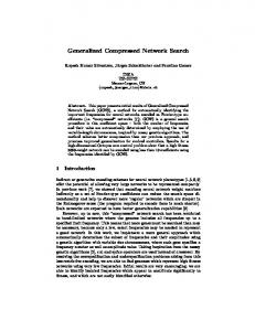
Fig. 1. Decoding the compressed networks. The figure shows the three step process involved in transforming a genome of frequency-domain coefficients into a recurrent neural network. First, the genome (left) is divided into k chromosomes, one for each of the weight matrices specified by the network architecture, Ψ. Each chromosome is mapped, by Algorithm 1, into a coefficient array of a dimensionality specified by Ω. In this example, an RNN with two inputs and four neurons is encoded as 8 coefficients. There are k = |Ω| = 3, chromosomes and Ω = {3, 3, 2}. The second step is to apply the inverse DCT to each array to generate the weight values, which are mapped into the weight matrices in the last step.

parsimonious solutions. CNCS maintains a probability distribution over complexity classes, which it uses to select which class to optimize. The probability of a given class is adapted based on the expected fitness of individuals sampled from it. Starting with a prior biased toward the simplest networks, the distribution adapts gradually until a solution is found. The idea of enforcing parsimony in neuroevolution has been explored previously [15, 16], usually by adding a regularization term to the fitness function that penalizes complexity. Our approach is more in line with NEAT [10] where simple networks are favored by starting evolution with a population of directly encoded networks that have minimal topologies. The next section describes how networks are encoded in the frequency domain. Section 3, introduces the complexity search method, CNCS. Section 4, presents experiments applying CNCS to the octopus arm task with high-dimensional actions to determine the number of coefficient genes used to represent networks; and in section 5 it is used to search for both the number of neurons (topology) and coefficients, for networks controlling a challenging version of the Helicopter Hovering benchmark.

2

DCT Network Representation

Networks are encoded as a string or genome, g = {g1 , . . . , gk }, consisting of k substrings or chromosomes of real numbers representing Discrete Cosine Transform (DCT) coefficients. The number of chromosomes is determined by the choice of network architecture, Ψ, and data structures used to decode the genome, specified by Ω = {D1 , . . . , Dk }, where Dm , m = 1..k, is the dimensionality of the coefficient array for chromosome m. The total number of coefficients, Pk C = m=1 |gm |  N (where N is the number of weights), is user-specified (for

Algorithm 1: Coefficient mapping(g, d)

p3 d3

d1

d2

p1

j ←0 K ← sort(diag(d) − I) P|d| for i = 0 to |d| − 1 + n=1 dn do l←0 P|d| si ← {e| k=1 eξj = i} while |si | > 0 do

ind[j] ← argmin e − K[l++ mod |d|] e∈si

p2

si ← si \ ind[j ++] for i = 0 to |ind| do if i < |g| then coeff array[ind[i]] ← ci else coeff array[ind[i]] ← 0

Fig. 2. Mapping the coefficients. The cuboidal array is filled with the coefficients 1 from chromosome g one simplex at a time, according to Algorithm 1, starting at the origin and moving to the opposite corner one simplex at a time.

a compression ratio of N/C), and the coefficients are distributed evenly over the chromosomes. Which frequencies should be included in the encoding is unknown. The approach taken here restricts the search space to band-limited neural networks where the power spectrum of the weight matrices goes to zero above a m specified limit frequency, cm ` , and chromosomes contain all frequencies up to c` , m m gm = (c0 , . . . , c` ). Figure 1 illustrates the procedure used to decode the genomes. In this example, a fully-recurrent neural network (on the right) is represented by k = 3 weight matrices, one for the input layer weights, one for the recurrent weights, and one for the bias weights. The weights in each matrix are generated from a different chromosome which is mapped into its own Dm -dimensional array with the same number of elements as its corresponding weight matrix; in the case shown, Ω = {3, 3, 2}: 3D arrays for both the input and recurrent matrices, and a 2D array for the bias weights. In previous work [5], the coefficient matrices were 2D, where the simplexes are just the secondary diagonals; starting in the top-left corner, each diagonal is filled alternately starting from its corners. However, if the task exhibits inherent structure that cannot be captured by low frequencies in a 2D layout, more compression can potentially be gained by organizing the coefficients in higher-dimensional arrays. Each chromosome is mapped to its coefficient array according to Algorithm 1 which takes a list of array dimension sizes, d = (d1 , . . . , dDm ) and the chromosome, gm , to create a total ordering on the array elements, eξ1 ,...,ξDm . In the first loop, the array is partitioned into (Dm −1)-simplexes, where each simplex, si , contains only those elements e whose Cartesian coordinates, (ξ1 , . . . , ξDm ), sum to integer i. The elements of simplex si are ordered in the while loop according to their distance to the corner points, pi (i.e. those points having exactly one non-zero coordinate; see example points for a 3D-array in figure 2), which form the rows of matrix K = [p1 , . . . , pm ]T , sorted in descending order by their sole, non-zero dimension size. In each loop iteration, the coordinates of the element

Algorithm 2: CNCS(D,f ,s,n,σθ ) while ¬converged do for k = 1 to s do xk ∼ D (µxk , σ xk ) ← SNES(f ,µxk , σ xk , λ(Ck ), n) φxk ← f (µxk ) foreach xi ∈D do   X 1 xi −xj   φx j d K max(σxi) > σθ h h g(xi ) ← ∀xj ∈D   0 otherwise foreach xi ∈ D do g(x ) p(xi ) ← X i g(xj )

//draw sample //store fitness

//normalize

∀xj ∈D

with the smallest Euclidean distance to the selected corner is appended to the list ind, and removed from si . The loop terminates when si is empty. After all of the simplexes have been traversed, the vector ind holds the ordered element coordinates. In the final loop, the array is filled with the coefficients from low to high frequency to the positions indicated by ind; the remaining positions are filled with zeroes. Finally, a Dm −dimensional inverse DCT transform is applied to the array to generate the weight values, which are mapped to their position in the corresponding 2D weight matrix. Once the k chromosomes have been transformed, the network is complete.

3

Compressed Network Complexity Search

The basic idea of CNCS is to discover networks with minimal complexity by running multiple independent evolutionary processes in parallel, one for each complexity class, allocating run-time to each according to an adaptive probability mass function, D. Algorithm 2 describes CNCS in pseudocode. The algorithm is initialized with a prior distribution over the complexity classes (C, Ψ ), where C is the number of coefficients used to encode the network, and Ψ is the number of neurons (equivalently, the topology). In order to bias the search toward low-complexity solutions, D should be initialized with a prior that gives high probability to small networks (low Ψ ), represented by the fewest number of coefficients (low C). Each xι = (Cι , Ψι ) pair in D has its own dedicated search algorithm used to optimize that particular configuration. In the current implementation we use Separable Natural Evolution Strategies (SNES; [13]), an efficient variant in the NES [12] family of black-box optimization algorithms. In each generation, SNES samples a population of λ individuals, computes a Monte Carlo estimate of the fitness gradient, transforms it to the natural gradient and updates the search distribution parameterized by a mean vector, µ, and diagonal covariance matrix, σ (see [12] for a full description of NES). The SNES search distribution associated with configuration xι has mean µxι and covariance σ xι .

32x32 recurrent connections

t tpu ou des no

32 nodes (11x3 grid, 1 not used)

32 outputs

82 inputs 32 bias weights

uts inp ar

ta 8s

v te

les iab

p om rc pe

ar

tm

t

en

base rotation + 10 compartments

(a)

(b)

Fig. 3. Octopus arm task. (a) A flexible arm consisting of p compartments, each with 3 muscles, must be controlled to touch a goal location with the arm tip from 3 different initial positions, −π/2, 0 and π/2. (b) The arm is controlled by a fully recurrent network with 32 neurons, one for each action (muscle). This topology is fixed, and only the number of coefficients used to represent its weights is determined automatically by CNCS.

Each iteration, CNCS draws s samples from D, and runs the SNES corresponding to each sample for n generations, after which the search distribution (µ, σ) and its expected fitness value φ are saved. The distribution D is then reestimated using a multivariate Parzen window estimator with radial-symmetric Gaussian kernel K [8]. First, the values g(x) are computed by applying the kernel weighted by the normalized fitnesses, φxj (the first forall loop), where h is the kernel width, and d is the dimensionality of D, e.g. 2 when estimating C and Ψ (the SNES distributions that have converged, max(σ) ≤ σθ , are assigned a g value of 0). Then the g values are normalized into probabilities, and the cycle repeats. The algorithm terminates when all search distributions (within the bounds of D) have converged, or either the desired fitness or the maximum number of iterations has been reached.

4

Octopus Arm Control

The octopus arm consists of p compartments floating in a 2D water environment (see figure 3a). Each compartment has a constant volume and contains three controllable muscles (dorsal, transverse and ventral). The goal of the task to reach a target position with the tip of the arm, starting from three different initial positions, by contracting the appropriate muscles at each 1s step of simulated time. While initial positions −π/2 and π/2 look symmetrical, they are actually quite different due to gravity. The state of a compartment is described by the x, y-coordinates of two of its corners plus their corresponding x and y velocities. Together with the arm base rotation, the arm has 8p + 2 state variables. Though there are 3p + 2 muscles, the task is normally simplified by aggregating them into 8 “meta”-actions that contract groups of muscles simultaneously (i.e. all dorsal, all transverse, etc.). Here, instead we use the more difficult configuration where the “raw” actions are controlled directly, so that each muscle must be coordinated with the others to move the arm.

input

input

p+1

12 muscle 1

muscle 2

8 state variables

muscle 3

n

p+1

recurrent

p+1

recurrent

bias

n

1

output

bias

n

1

n

3 muscles p+1

bias

p+1 4

3 muscles

(a) Octopus

(b) Helicopter

Fig. 4. Network decoding schemes. (a) for the octopus arm networks the genome is split into 3 chromosomes, Ω={4, 4, 2}. The coefficients in the chromosome used to generate the input weight matrix are placed in a 4D array, and a 2D array for the bias weights. (b) for the helicopter networks there are 5 chromosomes, Ω={2, 2, 1, 2, 1}: a 2D input and recurrent and output arrays, and 1D arrays for the input and output bias weights.

4.1

Setup

For the p = 10 compartment arm used in these experiments, a network with 32 neurons (one for each raw action) is sufficient to perform well on this task. Therefore, CNCS is used only to search for the number of coefficients, so that the distribution, D, is one-dimensional, with a uniform prior over C = 1..10, a sample size of s = 1, and number of SNES generations per CNCS update, n = 1. The kernel width was h = 7, and the convergence condition was set to σθ = 0.01. Each SNES used a population size of 16. Five experiments were run, for 4 thousand iterations each. The octopus arm was controlled using the fully-recurrent network architecture shown in figure 3b which is decoded using the following scheme, Ω= {4, 4, 2}, depicted in figure 4a: the genome is partitioned into k = 3 chromosomes, mapped into three arrays: (1) a 4D 8×(p+1)×3×(p+1) array that contains input weights for a 3×(p+1) grid of neurons, one for each raw action, (2) a 3×(p+1)×3×(p+1) recurrent weight array, and (3) and a 3×(p+1) bias array. The dimension size of 3 in these arrays refers to the number of muscles per compartment. The fitness as the average of the following score over three   wasd computed , 0 , where t is the number of time steps before the arm trials: max 1 − Tt D touches the goal, T is the maximum number of time steps in a trial, d is the final distance of the arm tip to the goal and D is the initial distance of the arm tip to the goal. Each of the three trials starts with the arm in a different configuration (see figure 3a). This fitness measure is different to the one used in [14], because minimizing the integrated distance of the arm tip to the goal causes greedy behaviors. In the viscous fluid environment of the octopus arm, a greedy strategy using the shortest length trajectory does not lead to the fastest movement: the

(a)

(b)

Fig. 5. Octopus arm results. The 3D plots show how (a) the distribution over the number of coefficients, C, adapts over time in CNCS, and (b) configurations with a better fitness are explored. The final distribution after 4,000 iterations is focused between C = 15 and C = 50, and peaks at C = 18, for a compression ratio of 204:1; 3680 weights/18 coefficients and fitness reaching 0.88.

arm has to be compressed first, and then stretched in the appropriate direction. Our fitness function favors behaviors that reach the goal within a small number of time steps. 4.2

Results

Figure 5 shows how the distribution (a) over coefficients, C, and the fitness of each configuration (b) adapts over the course of 4, 000 iterations of CNCS (averaged over 20 runs). The distribution is initialized with a prior that favors networks with low complexity, expressed solely with C (top-right corner of the graphs). The expected fitness forms a ridge with a peak between C = 15 and C = 18 with a moderate slope on the left, towards higher C. This focuses the search between C = 15 and C = 50. The expected fitness for C < 15 drops significantly lowering the probability of sampling configurations in this area. Reasonable fitness of 0.75 was reached at iteration 350 using less than 15 coefficients. A fitness of 0.88 that is close to optimum was reached at iteration 2560 using 18 coefficients. The weight matrices of such networks were compressed down from 3680 weights (compression ratio of 204:1).

5

Helicopter Hovering with Gusting Wind

The standard Helicopter Hovering benchmark involves maintaining the position of a simulated XCell Tempest [1] as close as possible to origin of a bounded 3D space (see figure 6a). The helicopter model consists of 12 state variables: the coordinates and angular rotations in 3-space and their derivatives; and 4 control variables: longitudinal and latitudinal cyclic pitch and tail, and main rotor collective pitch. The fitness is the sum of squares of all state variables over the course of a flight lasting t time steps. If the helicopter moves more that 20m away from the origin in any direction or its velocity exceeds 5 m/s, then it is

t tpu ou des o n

z

x

n de hid des no

4 outputs

n x n recurrent connections

4 bias weights n nodes

y 12 inputs n bias weights

inp

(a)

uts 12 helicopter state variables

(b)

Fig. 6. Helicopter hovering task with gusting wind. (a) The helicopter must be controlled to stay within 20m from its initial position at the origin (as shown). Unlike the standard version of the task where wind blows at a constant velocity, the wind here blows in gusts with much higher velocity, forcing the controller to react quickly to sudden changes in wind. (b) The helicopter is controlled by a simple recurrent network (SRN). Both the number of neurons and the number of coefficients are determined automatically by CNCS.

considered to have crashed, and the trial is terminated. The fitness is normalized between 0 and 1 and the minimum over 5 trials is used. The original 2008 RL competition version of this problem featured wind along the x- and y-axes with a drag of up to 5m/s, which is initialized at random in the beginning of each trial. With this setup, it turns out that a linear controller can be easily trained to solve the task. Therefore, in order to make the task more challenging, requiring non-linear control, the original wind model was modified so that instead of constant wind, strong “gusts” buffet the helicopter at random. Wind gusts occur in both x and y directions with probability 0.4 and a velocity of 20m/s, which decays exponentially after striking the helicopter. The gusting wind makes the task significantly harder—a linear controller cannot cope with the abrupt wind perturbations. Because higher velocities are required to control the helicopter under these conditions, the limit on the velocity was removed.

5.1

Setup

The helicopters were controlled using simple recurrent networks (SRN/Elman; figure 6b). The decoding scheme for the genomes, Ω= {2, 2, 1, 2, 1}, is depicted in figure 4b. The original benchmark involves flights of t = 6000 time steps (equivalent to 60s flight). For the task with gusting wind used here, this was reduced to 100 both for efficiency, and because, due to the severity of the wind, such a short trial is enough to evaluate relative controller competence. CNCS was used to search for both the network topology, Ψ (number of neurons), and number of coefficients, C. The complexity distribution, D, was initialized with a uniform prior over the range {1, 2} for both Ψ and C, i.e. p(C, Ψ ) = 0.25, C, Ψ = 1, 2, and a sample size s = 2. As in the octopus task, h = 7, σθ = 0.01, n = 1, and each SNES used a population size of 16. A total of 20 experiments were run, for 20 thousand iterations each.

Neurons 0

10 0

10 0

10 0

10 0

10 0

10

0

10 0

10 0

10 0

10 0

10 0

10

Coefficients

0

0 40

10

0

1

50

200

1000

5000

20 000 10 CNCS evaluations

1

50

200

1000

5000

20 000

Fig. 7. Complexity search distribution for helicopter hovering task. The figure shows how the distribution D (left) and fitness (right) evolve over time, averaged across 20 runs. The algorithm first explores simple networks, with only a few neurons, represented by a small number of DCT coefficients (around 500 steps), then gradually spreads the distribution toward more complex configurations, identifying two clusters with high fitness (networks with 3 neurons defined with 8 coefficients and 3-node networks defined with 12 coefficients).

5.2 Results Figure 7 shows how the distribution over (Ψ, C) configurations (top row) and the fitness of each configuration (bottom row) adapts over the course of 20k iterations of CNCS (averaged over 20 runs). The distribution is initialized with a prior that concentrates on networks with the lowest complexity (upper-left corner of the graphs). Gradually, as the distribution expands, it finds high fitness individuals with 1 to 3 neurons, using ≈ 8 coefficients, at around iteration 1000. These networks are simple both in terms of their topology (model complexity) and in the regularity of their weight matrices (compression ratio of 8:1, 64 weights/8 coefficients). The distribution then focuses on this area, moving away from configurations with fewer coefficients (C < 8) as they cannot express the level of complexity required for nets with more that 3 neurons. At this point, the distribution begins to follow a narrow, high-fitness corridor, adding coefficients to networks with 2 and 3 neurons, until it reaches C = 12 (≈ 2000 iterations) and starts to grow the size of networks. The shape of the distribution at 20k iterations emerged consistently for all runs, with a maximum relative entropy between the distributions of any two runs of only 0.038.

6

Discussion and Future Work

CNCS consistently found low-complexity solutions for the two tasks tested. The octopus arm reaching task was successfully solved with networks having 3680 weights that were generated using just 18 DCT coefficients, and networks with 2 neurons (64 weights) represented by 8 DCT coefficients were found in the early stage of the CNCS for the Helicopter Hovering task. Helicopter networks were progressively improved by increasing the number of DCT coefficients beyond 12, and broadening the search to more hidden neurons. The experimental results show that updating the distribution on complexity classes elegantly addresses the question of how to configure the evolution-

ary search. Running all configurations in parallel would be prohibitive, whereas CNCS quickly adapts the search distribution towards promising configurations. A potential drawback of CNCS lies in wide valleys of low fitness that span across complexity space. One has to ensure, that the width of the smoothing kernel used is wider than the potential valley. Otherwise, the distribution will never reach across to sample networks of higher complexity. A possible solution could be to use a variable kernel width for each complexity class based on e.g. the number of samples evaluated from that class. Future experiments will test the generalization of the evolved controllers to verify whether complexity is correlated with robustness. We expect that the small networks, although they have slightly worse fitness during the training (like those small networks that can control the helicopter to hover), will generalize better.

7

Acknowledgments

This research was funded by SNF grant 200020-125038/1.

References 1. P. Abbeel, V. Ganapathi, and A. Y. Ng. Learning vehicular dynamics, with application to modeling helicopters. In NIPS, 2005. 2. P. D¨ urr, C. Mattiussi, and D. Floreano. Neuroevolution with analog genetic encoding. In Proceeding of PPSN, pages 671–680, 2006. 3. F. Gruau. Cellular encoding of genetic neural networks. Technical Report RR-9221, Ecole Normale Superieure de Lyon, Institut IMAG, Lyon, France, 1992. 4. H. Kitano. Designing neural networks using genetic algorithms with graph generation system. Complex Systems, 4:461–476, 1990. 5. J. Koutn´ık, F. Gomez, and J. Schmidhuber. Evolving neural networks in compressed weight space. In Proceedings of the Conference on Genetic and Evolutionary Computation (GECCO-10), 2010. 6. J. Koutn´ık, F. Gomez, and J. Schmidhuber. Searching for minimal neural networks in fourier space. In Proc. of the 4th Conf. on Artificial General Intelligence, 2010. 7. L. A. Levin. Universal sequential search problems. Problems of Information Transmission, 9(3):265–266, 1973. 8. E. Parzen. On estimation of a probability density function and mode. The Annals of Mathematical Statistics, 33(3):pp. 1065–1076, 1962. 9. J. Schmidhuber. Discovering neural nets with low Kolmogorov complexity and high generalization capability. Neural Networks, 10(5):857–873, 1997. 10. K. O. Stanley and R. Miikkulainen. Evolving neural networks through augmenting topologies. Evolutionary Computation, 10:99–127, 2002. 11. K. O. Stanley and R. Miikkulainen. A taxonomy for artificial embryogeny. Artificial Life, 9(2):93–130, 2003. 12. D. Wierstra, T. Schaul, J. Peters, and J. Schmidhuber. Natural Evolution Strategies. In Proceedings of the Congress on Evolutionary Computation (CEC08), Hongkong. IEEE Press, 2008. 13. D. Wierstra, T. Schaul, T. G. Y. Sun, and J. Schmidhuber. Natural evolution strategies. Technical report, arXiv:1106.4487v1, 2011. 14. B. G. Woolley and K. O. Stanley. Evolving a single scalable controller for an octopus arm with a variable number of segments. In Proceedings of PPSN, pages 270–279, 2010. 15. B.-T. Zhang and H. Muhlenbein. Evolving optimal neural networks using genetic algorithms with Occam’s razor. Complex Systems, 7:199–220, 1993. 16. B.-T. Zhang and H. Muhlenbein. Balancing accuracy and parsimony in genetic programming. Evolutionary Computation, 3:17–38, 1995.