high-dimensional Octopus arm control problem show that a high fitness ..... the lower curve is for the lesioned case where the 13 most common frequency.
Generalized Compressed Network Search Rupesh Kumar Srivastava, J¨ urgen Schmidhuber and Faustino Gomez IDSIA USI-SUPSI Manno-Lugano, CH {rupesh,juergen,tino}@idsia.ch
Abstract. This paper presents initial results of Generalized Compressed Network Search (GCNS), a method for automatically identifying the important frequencies for neural networks encoded as Fourier-type coefficients (i.e. “compressed” networks [7]). GCNS is a general search procedure in this coefficient space – both the number of frequencies and their value are automatically determined by employing the use of variable-length chromosomes, inspired by messy genetic algorithms. The method achieves better compression than our previous approach, and promises improved generalization for evolved controllers. Results for a high-dimensional Octopus arm control problem show that a high fitness 3680-weight network can be encoded using less than 10 coefficients using the frequencies identified by GCNS.
1
Introduction
Indirect or generative encoding schemes for neural network phenotypes [1,5,6,9] offer the potential of allowing very large networks to be represented compactly. In previous work [7], we showed that encoding neural network weight matrices indirectly as a set of Fourier-type coefficients can reduce the search space dimensionality and help to discover more ‘regular’ networks which are simpler in the Kolmogorov sense (the program required to encode them is much shorter). Such networks are expected to have better generalization capabilities [9]. However, up to now, this “compressed” network search has been restricted to band-limited networks where the genome includes all frequencies up to a specified limit frequency. This means that more genes must be searched than may be necessary, because only a few, select frequencies may be needed to represent a good network. In this work, we implement a more general approach which automatically determines the subset of frequencies and their amplitudes using a genetic algorithm with variable size chromosomes, where each gene specifies a frequency number as well as amplitude value. Taking inspiration from the messy genetic algorithms [2], cut and splice operators are used instead of crossover. By resolving the overspecification and underspecification problems arising from this less restrictive encoding, we are able to find genomes which represent high fitness networks using very few frequencies. Initial results are very encouraging: we are able to identify isolated frequencies which appear to contribute significantly to fitness, and which are not easily identified otherwise.
Inverse DCT
(a)
Inverse DCT
(b) Inverse DCT
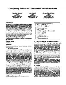
(c) Fig. 1. DCT network representation. The left column shows three different types of 2D frequency-domain coefficient arrays. The coefficients are arranged along the second diagonals, going from upper-left corner, to the bottom right corner. Each diagonal is filled from the edges to the center starting on the side that corresponds to the longer dimension. The right column shows the weight matrix resulting from applying the inverse DCT transform; gray-scale levels denote the weight values (black = low, white = high). In (a) all frequencies are present, so that all possible weight matrices can be represented. (b) Shows a band-limited weight matrix where only the first four coefficients from (a) are used, as in [7]. The weights in (b) are more spatially correlated than those in (a). (c) Shows a weight matrix encoded by a subset of frequencies from (a). GCNS searches this space of coefficient subsets (power set) of (a).
2
DCT Network Representation
The Discrete Cosine Transform (DCT) representation for neural networks, first introduced in [8], encodes network weight matrices in the frequency domain by using genomes of DCT coefficients. The motivation is that if weights that are near each other in the matrix are correlated, then the representation of the matrix in the frequency domain should require fewer parameters (coefficients1 ) than the number of weights in the matrix, thereby reducing the dimensionality of the search space. In this paper, all of the networks are fully connected recurrent neural networks (FRNNs) with i inputs, and single layer of n neurons where some of the neurons are treated as output neurons. An FRNN consists of three weight matrices: an n × i input matrix, I, an n × n recurrent matrix, R, and a bias vector t of length n. These three matrices are combined into one n × (n + i + 1) matrix, and 1
In this paper, we will use the terms ‘frequency’ and ‘coefficient’ interchangeably. To be precise, every frequency is associated with a coefficient which expresses its energy content.
`
index value
4 5.65
78
0 12
2.32 6.52
7 12 45
12.1 2.10 3.46
5.4
0
97 5
7.38 3.98 1.87
Fig. 2. GCNS coefficient genome. Each gene consists of two entries, the index of the DCT coefficient in the coefficient array, and the value of the coefficient. The same index can appear more than once in the genome, and genomes have variable length, `.
encoded indirectly using c ≤ N DCT coefficients, where N is the total number of weights in the network. Figure 1 illustrates the relationship between the coefficients and weights for a hypothetical 4 × 6 weight matrix (e.g. a network with four neurons each with six weights). The left side of the figure shows three weight matrix encodings that use different coefficients. Generally speaking, coefficient ci is considered to be more significant (associated with a lower frequency) than cj , if i < j. The right side of the figure shows the weight matrices that are generated by applying the inverse DCT transform to the coefficients. In the first case (a), all 24 coefficients are used, so that any possible 4×6 weight matrix can be represented. The particular weight matrix shown was generated from random coefficients in [−20, 20]. In (b), each ci has the same value as in (a), but the full set has been truncated up to the first four lowest frequencies, favoring smoother matrices. This is the approach taken in [7] where a limit frequency c` (c4 in the example) is specified by the user, and genomes of length ` are evolved. In (c), the coefficient matrix again has only four non-zero coefficients, but the coefficients are not restricted to a band-limited spectrum; they can be at any frequency. The genomes evolved by GCNS search this less constrained space.
3
Generalized Compressed Network Search
Generalized Compressed Network Search (GCNS) attempts to simultaneously find the number of coefficients required to represent a high fitness network, their indices (2D frequency), and their values. Variable size chromosomes are used where each gene has two elements: the coefficient index and the value (see figure 2). The coefficient index determines the position of the coefficient in the coefficient matrix which is transformed into the network via the inverse DCT. The overspecification problem (some genes can have multiple copies in the genome) is handled as in messy genetic algorithms [2, 3]. If a coefficient index appears multiple times in a genome, only its first value, reading from left to right, gets expressed in the phenotype. This results in an intra-chromosomal dominance operator. The problem of underspecification (some of the frequencies do not appear in a particular genome) elegantly resolves itself due to the nature of the encoding: if a particular coefficient number does not appear in the genome, it is muted in the phenotype i.e. its value is taken to be zero. GCNS starts with an initial parent population of size popsize with genomes of variable lengths containing frequency indices and values randomly chosen in a
Fig. 3. Cut and Splice. This schematic shows the effect of application of the cut and splice operators on a set of two parent genomes. In the case shown, only P1 gets cut resulting in three chromosomes (strands S1, S2 and parent P2). Then splice is applied with probability ps . If the first splice succeeds, then S1 gets spliced with P2, leaving S2 as a separate genome. If first splice does not occur, another splice between S2 and P2 can lead to the two children shown if it succeeds. If both splices do not succeed, S1, S2 and P2 become the final children as shown. Similar possibilities exist for other cases of the parents getting cut.
given range. At each generation, the child population is formed from the parent population by applying the ‘cut’ and ‘splice’ operators in groups of two to randomly chosen members from the parent population (without replacement). The process of applying cut and splice is a generalization of the crossover operation to the variable length genome case, and can yield one to four children from two parents. First, it is determined whether one, both or none of the two parents will be cut. The probability of cut is given by pc ∗ (l − 1) where l is the length of the genome and pc is a parameter. The location of the cut on a genome is randomly chosen over its length. At this intermediate step, there are two to four chromosomes present depending on the number of cuts that occur. The splice operator then joins together pairs of chromosomes with probability ps , resulting in either one (splice succeeds) or two (splice fails) children for each splice. Figure 3 shows the recombination of the parent genomes in an example scenario. As shown, when only parent 1 is cut, three possible sets of children can result after splicing. The other scenarios are handled similarly. After cutting and splicing, mutation is applied to each coefficient index (with probability pmi ) and value (with probability pmv ) by drawing new values from Gaussian distributions centered at their current values and having fixed standard deviations. The value of pmi is kept much lower than pmv so that new frequencies are introduced only sporadically, allowing the algorithm to focus on refining the selected coefficients. In all our runs, the standard deviations were taken to be 5 and 10 for the indices and values, respectively. After all the children have been evaluated, the best popsize members from the combined parent and child populations are chosen as the parents for the next generation. The algorithm terminates after the specified number of generations.
32x32 recurrent connections
t tpu ou des no
32 nodes (11x3 grid, 1 not used)
32 outputs
82 inputs 32 bias weights
uts inp ar
ta 8s
v te
les iab
p om rc pe
ar
tm
t
en
base rotation + 10 compartments
(a)
(b)
Fig. 4. Octopus arm task. (a) A flexible arm consisting of p compartments, each with 3 muscles, must be controlled to touch a goal location with the arm tip from the −π/2 position. The other two standard, initial positions were not used (see text). (b) The arm is controlled by a fully recurrent network with 32 neurons, one for each action (muscle). This topology is fixed, and only the number of coefficients used to represent its weights is determined automatically by GCNS.
4
Octopus arm control
The octopus arm consists of n compartments floating in a 2D water environment [10]. Each compartment has a constant volume and contains three controllable muscles (dorsal, transverse and ventral). The state of a compartment is described by the x, y-coordinates of two of its corners plus their corresponding x and y velocities. Together with the arm base rotation, the arm has 8n + 2 state variables and 3n + 2 control variables. The goal of the task is to reach a goal position with the tip of the arm, starting from different initial positions, by contracting the appropriate muscles at each 1s step of simulated time. The standard setup uses 3 initial positions (figure 4); here, only one initial position was used for training (the arm starts hanging straight down), since it turns out the other two (indicated in gray, figure 4) are very easy to solve, and successful networks tend to generalize to them. The fitness function is given by (1 − (t ∗ d)/(T ∗ D)) where t is the number of time steps taken to reach the goal, d is final arm tip distance to the goal, T maximum the number of time steps in a trial, and D is the initial arm tip distance to the goal.
4.1
Setup
GCNS was run 30 times with popsize = 100, ngen = 150, pc = 0.2, ps = 0.8, pmi = 0.1 and pmv = 0.8. The initial population contained genomes of random length, `, ranging from 2 to 20 genes, with indices chosen at random from [1, 100], and values chosen at random from [−30, 30]. With this setup, no one genome contains all of the 100 available frequencies, but with very high probability all frequencies are present in the population.
8p+2
n
1
n
input
rec. bias
Fig. 5. Coefficient matrix. There is one coefficient matrix for all of the weights in the network. The small boxes in the upper left-hand corner denote coefficients organized in the usual way (as in [4, 7]) in the matrix, from this corner to the opposite corner, in order of increasing frequency. In GCNS, genomes can instead contain frequencies from anywhere in the (bounded) spectrum (denoted by gray boxes), without having to include all lower frequencies. When the iDCT is applied to this matrix, a matrix of weights of the same size is generated, and sliced into three sub-matrices (indicated by vertical lines): one for the input weights, one for the recurrent weights, and a bias vector.
4.2
Results
The mean best fitness over 30 runs was 0.95, while the average number of expressed genes (i.e. non-dominated) in the best genomes was 9.8, one-third the number required in [7] to achieve similar fitness. It is important to point out that our objective here is not to demonstrate raw performance, but to determine whether a small basis (set of frequencies) can be discovered and parameterized consistently. Figure 6 shows how the frequency content in the population declines over the course of evolution as the search converges to just a few frequencies for the behavior of a typical run. Interestingly, we found that in addition to the fundamental frequency (index 1, which we expected), almost all of the most fit networks contained either index 84 or 97, with large values. The 2D cosine functions represented by these indices seem to capture a basic regularity inherent in the task, given the network architecture used. Figure 9 shows the weight matrices of three difference networks with high fitness and their GCNS genomes. All three have a very regular structure. The third network (figure 9c) can be completely specified with just 10 numbers, for a compression ratio of 3680/10 = 368. 4.3
Lesion study
In order to determine whether the frequencies that were found consistently in highly fit networks are somehow “special” in that it is easier to find good values for them, the experiments were run again, but this time the frequencies occurring most often in the final populations of the previous experiments (indices: 0, 1, 2, 3, 5, 15, 17, 28, 31, 51, 71, 83, 96) were not allowed to be expressed (figure 7, top). Any time one of these frequencies occurred in a genome its value was muted by setting it to zero. Figure 8, compares the performance of GCNS using these lesioned genomes versus the unlesioned genomes in the first experiments. Without access to the
400 350 300
Gen 0
250 200 150
No. occurences in population
100 50 4000 350
Gen 50
300 250 200 150 100 50 4000 350 300 250 200 150 100 50 4000 350 300 250 200 150
Gen 100
640
Gen 150
100 50 0
0
20
40
60
Coefficient index
80
100
Fig. 6. Evolution of population frequency content. Each plot is a histogram of the coefficient indices (2D DCT frequencies) in the GCNS population of a typical run at particular point during evolution. In the initial random population (Gen 0), each frequency occurs about as often as any other. By generation 50 (Gen 50), about 20 frequencies have started to dominate the population.
lesioned frequencies, fitness improves more slowly reaching an average of 0.88. To do this, the lesioned runs are forced to use alternative frequencies (indices: 9, 10, 12, 21, 23, 60, 79, 87, 92, 94, 100; indicated in black in the bottom plot of figure 7) that take longer to set properly.
5
Discussion and Future Work
The indirect encoding of neural networks using Fourier-type coefficients is promising since this scheme can reduce the dimensionality of the search space by orders of magnitude and allow very compact representations of the networks. If a particular problem suggests that a high degree of redundancy is expected in the network, this encoding can efficiently exploit this regularity. This has been demonstrated previously by searching for a fixed set of frequencies [4, 7]. The present work aims to address some key issues of dealing with this encoding scheme. First, the previous study used a fixed set of contiguous frequencies to encode the networks. In one run, a set of coefficient values corresponding to these
200
630
Unlesioned
150
Avg. no. of occurrences
100
50
0 200
Lesioned 150
100
50
0
0
20
40
60
80
100
Coefficient index Fig. 7. Average frequency content in final populations. Each histogram shows the indices present in the final population averaged over the 30 runs. In the upper, unlesioned plot, the indices marked in black are those that cross the chosen threshold of 30 (horizontal line). These frequencies are muted in the lesioned runs (lower plot), where alternative solution indices emerge to compensate for those that are lesioned.
frequencies was identified. However, it is uncertain what is the number of frequencies sufficient to encode a high fitness network. Thus, several runs must be repeated with increasing number of frequencies to ensure that sufficiently high fitness networks can be found. Moreover, the sufficient set of frequencies for a particular problem may not consist of contiguous frequencies and thus a higher degree of compression is possible if this restriction of contiguity can be lifted. GCNS addresses both these issues: it restricts neither the number nor separation of the frequencies, and as expected, leads to higher compression. Although there is no explicit importance given to simpler representations (lesser number of unique frequencies) in GCNS, the cut and splice operators coupled with the elitist nature of the algorithm ensure that genomes become longer only if required. Thus, if a particular problem does not allow high compression, GCNS will utilize more frequencies until the complexity required can be expressed. Further research in this direction is underway.
6
Acknowledgments
This research was funded by the following EU projects: IM-CLeVeR (FP7-ICTIP-231722) and WAY (FP7-ICT-288551).
1 Unlesioned Lesioned
0.9
Fitness
0.8 0.7 0.6 0.5 0.4
0
20
40
60
80
Generations
100
120
140
Fig. 8. Performance on Octopus arm task. The plot shows the fitness of the best network in each generation, averaged of 30 runs, with 95% confidence intervals. The upper curve is for the unlesioned case where all 100 coefficients are active in the evolving genomes; the lower curve is for the lesioned case where the 13 most common frequency indices found in the final populations of the unlesioned runs are “muted”. Removing these frequencies from the set of available alleles slows down the search, forcing GCNS to find alternative solutions consisting of frequencies that are more difficult to set properly.
References 1. P. D¨ urr, C. Mattiussi, and D. Floreano. Neuroevolution with analog genetic encoding. In PPSN, pages 671–680, 2006. 2. D. Goldberg, B. Korb, and K. Deb. Messy genetic algorithms: Motivation, analysis, and first results. Complex systems, 3(5):493–530, 1989. 3. D. E. Goldberg, K. Deb, H. Kargupta, and G. Harik. Rapid, accurate optimization of difficult problems using fast messy genetic algorithms. In Proc. of the Fifth Intl. Conference on Genetic Algorithms, pages 56–64. Morgan Kaufmann, 1993. 4. F. Gomez, J. Koutn´ık, and J. Schmidhuber. Compressed network complexity search. In Proceedings of the 12th International Conference on Parallel Problem Solving from Nature (PPSN-XII), 2012. 5. F. Gruau. Cellular encoding of genetic neural networks. Technical Report RR-9221, Ecole Normale Superieure de Lyon, Institut IMAG, Lyon, France, 1992. 6. H. Kitano. Designing neural networks using genetic algorithms with graph generation system. Complex Systems, 4:461–476, 1990. 7. J. Koutn´ık, F. Gomez, and J. Schmidhuber. Evolving neural networks in compressed weight space. In Proc. of the 12th annual conference on Genetic and evolutionary computation, pages 619–626. ACM, 2010. 8. J. Koutn´ık, F. Gomez, and J. Schmidhuber. Searching for minimal neural networks in fourier space. In Proc. of the 4th Conf. on Artificial General Intelligence, 2010. 9. J. Schmidhuber. Discovering neural nets with low Kolmogorov complexity and high generalization capability. Neural Networks, 10(5):857–873, 1997. 10. Y. Yekutieli, R. Sagiv-Zohar, R. Aharonov, Y. Engel, B. Hochner, and T. Flash. Dynamic model of the octopus arm. I. Biomechanics of the octopus reaching movement. Journal of neurophysiology, 94(2):1443–1458, 2005.
n
(a)
o
21 31 47 57 84 1 6 8 10 11 13 18 19 29 41 72 97 2.74, 0.1, 6.29, 11.72, 10.41, 12.32, 9.5, 15.99, −31.65, 35.47, −35.59, 29.06, −26.79, −26.23, 16.98, −0.5, 72.82
� (b)
1
7
19
26
32
52
84
95
�
12.04, 10.65, 19.92, 20.06, 42.82, 49.27, 49.07, −43.49
� (c)
1
20
47
75
97
�
27.31, 22.52, −20.25, 36.34, 38.44
Fig. 9. Low-complexity weight matrices. Each row shows the weight matrices of a successful network (refer to figure 5 for a description of each sub-matrix). Colors indicate weight values. The genome used to generate the network is shown below each image.