Compressed Sensing Meets Machine Learning - Inst.eecs.berkeley.edu

`1 -Minimization

Introduction

`0 /`1 -Equivalence

Conclusion

Compressed Sensing Meets Machine Learning - Classification of Mixture Subspace Models via Sparse Representation Allen Y. Yang

Mini Lectures in Image Processing (Part II), UC Berkeley

Allen Y. Yang

< [email protected]>

Compressed Sensing Meets Machine Learning

`1 -Minimization

Introduction

`0 /`1 -Equivalence

Nearest Neighbor Algorithm

1 2

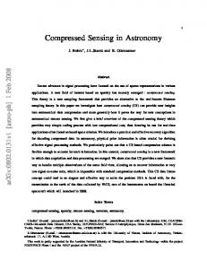
Training: Provide labeled samples for K classes. Test: Present a new sample Compute its distances with all training samples. Assign its label as the same label of the nearest neighbor.

Allen Y. Yang



Conclusion

`1 -Minimization

Introduction

`0 /`1 -Equivalence

Nearest Subspace Estimation of single subspace models Suppose R = [w1 , · · · , wd ] is a basis for a d-dim subspace in RD . For xi ∈ RD , its coordinate in the new coordinate system: wT xi = yi ∈ R.

Allen Y. Yang



Conclusion

`1 -Minimization

Introduction

`0 /`1 -Equivalence

Nearest Subspace Estimation of single subspace models Suppose R = [w1 , · · · , wd ] is a basis for a d-dim subspace in RD . For xi ∈ RD , its coordinate in the new coordinate system: wT xi = yi ∈ R. Principal component analysis w∗ = arg max w

Allen Y. Yang

n X

(yi )2 = arg max wT Σw

i=1



Conclusion

`1 -Minimization

Introduction

`0 /`1 -Equivalence


n X


i=1

Numerical solution: Singular value decomposition (SVD) svd(A) = USV T , where U ∈ RD×D , S ∈ RD×n , V ∈ Rn×n . Denote U = [U1 ∈ RD×d ; U2 ∈ RD×(D−d) ]. Then R = U1T .

Allen Y. Yang



Conclusion

`1 -Minimization

Introduction

`0 /`1 -Equivalence


n X


i=1

Numerical solution: Singular value decomposition (SVD) svd(A) = USV T , where U ∈ RD×D , S ∈ RD×n , V ∈ Rn×n . Denote U = [U1 ∈ RD×d ; U2 ∈ RD×(D−d) ]. Then R = U1T . Eigenfaces If xi are vectors of face images, the principal vectors wi are then called Eigenfaces.

Allen Y. Yang



Conclusion

`1 -Minimization

Introduction

`0 /`1 -Equivalence

Conclusion

Nearest Subspace Algorithm

1

Training: For each of K classes, estimate its d-dim subspace model Ri = [w1 , · · · , wd ].

2

Test: Present a new sample y, compute its distances to K subspaces.

3

Assignment: label of y as the closest subspace.

Allen Y. Yang



`1 -Minimization

Introduction

`0 /`1 -Equivalence

Conclusion

Nearest Subspace Algorithm

1

Training: For each of K classes, estimate its d-dim subspace model Ri = [w1 , · · · , wd ].

2

Test: Present a new sample y, compute its distances to K subspaces.

3

Assignment: label of y as the closest subspace.

Question Equation for computing distance from y to Ri ? Why NS likely outperforms NN?

Allen Y. Yang



`1 -Minimization

Introduction

`0 /`1 -Equivalence

Noiseless `1 -Minimization is a Linear Program Recall last lecture: Compute sparsest solution x that satisfies ˜ ∈ Rd ˜ y = Ax

Allen Y. Yang



Conclusion

`1 -Minimization

Introduction

`0 /`1 -Equivalence

Noiseless `1 -Minimization is a Linear Program Recall last lecture: Compute sparsest solution x that satisfies ˜ ∈ Rd ˜ y = Ax Formulate as linear programming: 1

Problem statement: (P1 ) :

Allen Y. Yang

˜ ∈ Rd x∗ = arg min kxk1 subject to ˜ y = Ax x



Conclusion

`1 -Minimization

Introduction

`0 /`1 -Equivalence

Conclusion

Noiseless `1 -Minimization is a Linear Program Recall last lecture: Compute sparsest solution x that satisfies ˜ ∈ Rd ˜ y = Ax Formulate as linear programming: 1


2

˜ ∈ Rd x∗ = arg min kxk1 subject to ˜ y = Ax x

˜ −A) ˜ ∈ Rd×2n , c = (1, 1, · · · , 1)T ∈ R2n . We have the following linear Denote Φ = (A, program w∗

Allen Y. Yang

= subject to


arg minw cT w ˜ y = Φw w≥0


`1 -Minimization

Introduction

`0 /`1 -Equivalence

`1 -Minimization Routines Matching pursuit [Mallat 1993] 1 2 3

˜ with y: i = arg max hy, vj i. Find most correlated vector vi in A ˜ ←A ˜ˆi , xi ← hy, vi i, y ← y − xi vi . A Repeat until kyk < .

Allen Y. Yang



Conclusion

`1 -Minimization

Introduction

`0 /`1 -Equivalence



Basis pursuit [Chen 1998] 1 2

Assume x0 is m-sparse. ˜ as a basis Select m linearly independent vectors Bm in A †

xm = Bm y. 3 4

˜ if improve ky − Bm xm k. Repeat swapping one basis vector in Bm with another vector in A If ky − Bm xm k2 < , stop.

Allen Y. Yang



Conclusion

`1 -Minimization

Introduction

`0 /`1 -Equivalence



Basis pursuit [Chen 1998] 1 2

Assume x0 is m-sparse. ˜ as a basis Select m linearly independent vectors Bm in A †

xm = Bm y. 3 4

˜ if improve ky − Bm xm k. Repeat swapping one basis vector in Bm with another vector in A If ky − Bm xm k2 < , stop.

Matlab Toolboxes SparseLab by Donoho at Stanford. cvx by Boyd at Stanford.

Allen Y. Yang



Conclusion

`1 -Minimization

Introduction

`0 /`1 -Equivalence

`1 -Minimization with Bounded `2 -Noise is Quadratic Programming `1 -Minimization with Bounded `2 -Noise: ˜ 0 + z ∈ Rd , where kzk2 < ˜ y = Ax

Allen Y. Yang



Conclusion

`1 -Minimization

Introduction

`0 /`1 -Equivalence



Allen Y. Yang

˜ 2


Conclusion

`1 -Minimization

Introduction

`0 /`1 -Equivalence



˜ 2


Conclusion

`1 -Minimization

Introduction

`0 /`1 -Equivalence



˜ 2


Conclusion

`1 -Minimization

Introduction

`0 /`1 -Equivalence

Recall last lecture... 1

`0 -Minimization ˜ x0 = arg min kxk0 s.t. ˜ y = Ax. x

k · k0 simply counts the number of nonzero terms.

Allen Y. Yang



Conclusion

`1 -Minimization

Introduction

`0 /`1 -Equivalence

Recall last lecture... 1

`0 -Minimization ˜ x0 = arg min kxk0 s.t. ˜ y = Ax. x

k · k0 simply counts the number of nonzero terms. 2

`0 -Ball `0 -ball is not convex. `0 -minimization is NP-hard.

Allen Y. Yang



Conclusion

`1 -Minimization

Introduction

`0 /`1 -Equivalence

`1 /`0 Equivalence 1

Compressed sensing: If x0 is sparse enough, `0 -minimization is equivalent to (P1 )

˜ min kxk1 s.t. ˜ y = Ax.

kxk1 = |x1 | + |x2 | + · · · + |xn |.

Allen Y. Yang



Conclusion

`1 -Minimization

Introduction

`0 /`1 -Equivalence




kxk1 = |x1 | + |x2 | + · · · + |xn |. 2

`1 -Ball

`1 -Minimization is convex. Solution equal to `0 -minimization.

Allen Y. Yang



Conclusion

`1 -Minimization

Introduction

`0 /`1 -Equivalence




kxk1 = |x1 | + |x2 | + · · · + |xn |. 2

`1 -Ball

`1 -Minimization is convex. Solution equal to `0 -minimization.

3

`1 /`0 Equivalence: [Donoho 2002, 2004; Candes et al. 2004; Baraniuk 2006] ˜ 0 , there exists equivalence breakdown point (EBP) ρ(A), ˜ if kx0 k0 < ρ: Given ˜ y = Ax `1 -solution is unique x1 = x0

Allen Y. Yang



Conclusion

`1 -Minimization

Introduction

`0 /`1 -Equivalence

`1 /`0 Equivalence in Noisy Case Reconsider `2 -bounded linear system ˜ 0 + z ∈ Rd , where kzk2 < ˜ y = Ax Is corresponding `1 solution stable?

Allen Y. Yang



Conclusion

`1 -Minimization

Introduction

`0 /`1 -Equivalence

`1 /`0 Equivalence in Noisy Case Reconsider `2 -bounded linear system ˜ 0 + z ∈ Rd , where kzk2 < ˜ y = Ax Is corresponding `1 solution stable? 1

`1 -Ball

No exact solution possible. Bounded measurement error causes bounded estimation error. Yes, `1 solution is stable!

Allen Y. Yang



Conclusion

`1 -Minimization

Introduction

`0 /`1 -Equivalence

Conclusion

`1 /`0 Equivalence in Noisy Case Reconsider `2 -bounded linear system ˜ 0 + z ∈ Rd , where kzk2 < ˜ y = Ax Is corresponding `1 solution stable? 1

`1 -Ball

No exact solution possible. Bounded measurement error causes bounded estimation error. Yes, `1 solution is stable!

2

`1 /`0 Equivalence [Donoho 2004] ˜ 0 + z where kzk2 < . There exists equivalence breakdown point (EBP) Suppose ˜ y = Ax ˜ if kx0 k0 < ρ: ρ(A), kx1 − x0 k2 ≤ C ·

Allen Y. Yang



`1 -Minimization

Introduction

`0 /`1 -Equivalence

Compressed Sensing in the View of Convex Polytopes For the rest of the lecture, investigate the estimation of EBP ρ. To simplify notations, assume underdetermined system y = Ax ∈ Rd , where A = Rd×n .

Allen Y. Yang



Conclusion

`1 -Minimization

Introduction

`0 /`1 -Equivalence

Compressed Sensing in the View of Convex Polytopes For the rest of the lecture, investigate the estimation of EBP ρ. To simplify notations, assume underdetermined system y = Ax ∈ Rd , where A = Rd×n . Definition (Quotient Polytopes) Consider the convex hull P of the 2n vectors (A, −A). P is called the quotient polytope associated to A.

Allen Y. Yang



Conclusion

`1 -Minimization

Introduction

`0 /`1 -Equivalence

Conclusion

Compressed Sensing in the View of Convex Polytopes For the rest of the lecture, investigate the estimation of EBP ρ. To simplify notations, assume underdetermined system y = Ax ∈ Rd , where A = Rd×n . Definition (Quotient Polytopes) Consider the convex hull P of the 2n vectors (A, −A). P is called the quotient polytope associated to A.

Definition (k-Neighborliness) A quotient polytope P is called k-neighborly if whenever we take k vertices not including an antipodal pair, the resulting vertices span a face of P. (Above example is 1-neighborly.)

Allen Y. Yang



`1 -Minimization

Introduction

`0 /`1 -Equivalence

`1 -Minimization and Quotient Polytopes Why `1 -minimization is related to quotient polytopes?

Consider x represent an `1 -ball C in Rn .

Allen Y. Yang



Conclusion

`1 -Minimization

Introduction

`0 /`1 -Equivalence


Consider x represent an `1 -ball C in Rn . If x0 is k-sparse, x0 will intersect the `1 -ball on one of its (k − 1)-D faces.

Allen Y. Yang



Conclusion

`1 -Minimization

Introduction

`0 /`1 -Equivalence


Consider x represent an `1 -ball C in Rn . If x0 is k-sparse, x0 will intersect the `1 -ball on one of its (k − 1)-D faces. Matrix A maps `1 -ball in Rn to the quotient polytope P in Rd , d n.

Allen Y. Yang



Conclusion

`1 -Minimization

Introduction

`0 /`1 -Equivalence


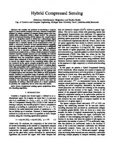
Consider x represent an `1 -ball C in Rn . If x0 is k-sparse, x0 will intersect the `1 -ball on one of its (k − 1)-D faces. Matrix A maps `1 -ball in Rn to the quotient polytope P in Rd , d n. Such mapping is linear!

Allen Y. Yang



Conclusion

`1 -Minimization

Introduction

`0 /`1 -Equivalence

Conclusion


Consider x represent an `1 -ball C in Rn . If x0 is k-sparse, x0 will intersect the `1 -ball on one of its (k − 1)-D faces. Matrix A maps `1 -ball in Rn to the quotient polytope P in Rd , d n. Such mapping is linear! Theorem (`1 /`0 equivalence condition) If the quotient polytope P associated with A is k-neighborly, for y = Ax0 with x0 to be k-sparse, then x0 is the unique optimal solution of the `1 -minimization.

Allen Y. Yang



`1 -Minimization

Introduction

`0 /`1 -Equivalence

Let’s prove the theorem together

Definitions: vertices v ∈ vert(P).

Allen Y. Yang



Conclusion

`1 -Minimization

Introduction

`0 /`1 -Equivalence


Definitions: vertices v ∈ vert(P). k-D faces F ∈ Fk (P). Also define fk (P) = #Fk (P).

Allen Y. Yang



Conclusion

`1 -Minimization

Introduction

`0 /`1 -Equivalence


Definitions: vertices v ∈ vert(P). k-D faces F ∈ Fk (P). Also define fk (P) = #Fk (P). convex hull operation conv(·). (1) vert(P) = F0 (P). (2) P = conv(vert(P))

Allen Y. Yang



Conclusion

`1 -Minimization

Introduction

`0 /`1 -Equivalence


Definitions: vertices v ∈ vert(P). k-D faces F ∈ Fk (P). Also define fk (P) = #Fk (P). convex hull operation conv(·). (1) vert(P) = F0 (P). (2) P = conv(vert(P)) F ∈ Fk (P) is a simplex if #vert(F ) = k + 1. Properties vert(AC ) ⊂ Avert(C );

Allen Y. Yang


Fl (AC ) ⊂ AFl (C ).


Conclusion

`1 -Minimization

Introduction

`0 /`1 -Equivalence

Two Fundamental Lemmas

Lemma (Alternative Definition of k-neighborliness) Suppose a centrosymmetric polytope P = AC has 2n vertices. Then P is k-neighborly iff for any l = 0, · · · , k − 1 and F ∈ Fl (C ), AF ∈ Fl (AC ).

Allen Y. Yang



Conclusion

`1 -Minimization

Introduction

`0 /`1 -Equivalence

Two Fundamental Lemmas

Lemma (Alternative Definition of k-neighborliness) Suppose a centrosymmetric polytope P = AC has 2n vertices. Then P is k-neighborly iff for any l = 0, · · · , k − 1 and F ∈ Fl (C ), AF ∈ Fl (AC ). Lemma (Unique Representation on Simplices) Consider an l-simplex F ∈ Fl (P). Let x ∈ F . Then 1

x has a unique representation as a linear combination of the vertices of P.

2

This representation places only nonzero weight on vertices of F .

Allen Y. Yang



Conclusion

`1 -Minimization

Introduction

`0 /`1 -Equivalence

Conclusion

Proof of the Theorem

Suppose P is k-neighborly, and x0 is k-sparse. WLOG, scale and assume kx0 k1 = 1. . 1 x0 is k-sparse ⇒ ∃F ∈ Fk−1 (C ), x0 ∈ F and y = Ax0 ∈ AF . 2

P = AC is k-neighborly ⇒ AF ∈ Fk−1 (AC ) is a simplex.

3

By (1) and (2), y ∈ AF has a unique representation with at most k nonzero weights on the vertices of AF .

4

Hence, x1 given by `1 -minimization is unique, and x1 = x0 .

Allen Y. Yang



`1 -Minimization

Introduction

`0 /`1 -Equivalence

Conclusion

Proof of the Theorem

Suppose P is k-neighborly, and x0 is k-sparse. WLOG, scale and assume kx0 k1 = 1. . 1 x0 is k-sparse ⇒ ∃F ∈ Fk−1 (C ), x0 ∈ F and y = Ax0 ∈ AF . 2

P = AC is k-neighborly ⇒ AF ∈ Fk−1 (AC ) is a simplex.

3

By (1) and (2), y ∈ AF has a unique representation with at most k nonzero weights on the vertices of AF .

4

Hence, x1 given by `1 -minimization is unique, and x1 = x0 .

Corollary [Gribonval & Nielsen 2003] Assume for all columns of matrix A, kvi k2 = 1, and for all i 6= j, hvi , vj i ≤ then P = AC is k-neighborly.

Allen Y. Yang


1 2k−1 ,


`1 -Minimization

Introduction

`0 /`1 -Equivalence

Last question: Why random projection works well in `1 -minimization?

Revisit the above corollary . Define coherence M = maxi6=j |hvi , vj i|, then EBP(A) >

Allen Y. Yang


M −1 +1 . 2


Conclusion

`1 -Minimization

Introduction

`0 /`1 -Equivalence


Revisit the above corollary . Define coherence M = maxi6=j |hvi , vj i|, then EBP(A) > 1

M −1 +1 . 2

in HD space Rd , two randomly generated unit vectors have small coherence M.

Allen Y. Yang



Conclusion

`1 -Minimization

Introduction

`0 /`1 -Equivalence

Conclusion


Revisit the above corollary . Define coherence M = maxi6=j |hvi , vj i|, then EBP(A) > 1 2

M −1 +1 . 2

in HD space Rd , two randomly generated unit vectors have small coherence M. Further define coherence of two dictionaries M(A, B) = maxu∈A,v∈B |hu, vi|. √1 d

≤ M(A, B) ≤ 1.

Let T be the spike basis in time domain, F be the Fourier basis, then M(T , F ) = incoherence! Random projection R in general is not coherent with most traditional bases.

Allen Y. Yang



√1 d

. Max

`1 -Minimization

Introduction

`0 /`1 -Equivalence

Conclusion 1

Classical classifiers: NN & NS.

2

Linear and quadratic `1 solvers.

3

Stability of `0 /`1 equivalence with bounded error.

4

Computation of equivalence breakdown point (EBP) via quotient polytopes.

Allen Y. Yang



Conclusion