Compressibility of Deterministic and Random Infinite ... - IEEE Xplore

IEEE TRANSACTIONS ON SIGNAL PROCESSING, VOL. 59, NO. 11, NOVEMBER 2011

5193

Compressibility of Deterministic and Random Infinite Sequences Arash Amini, Michael Unser, Fellow, IEEE, and Farokh Marvasti, Senior Member, IEEE

Abstract—We introduce a definition of the notion of compressibility for infinite deterministic and i.i.d. random sequences which is based on the asymptotic behavior of truncated subsequences. For this purpose, we use asymptotic results regarding the distribution of order statistics for heavy-tail distributions and their link with -stable laws for . In many cases, our proposed definition of compressibility coincides with intuition. In particular, we prove that heavy-tail (polynomial decaying) distributions fulfill the requirements of compressibility. On the other hand, exponential decaying distributions like Laplace and Gaussian do not. The results are such that two compressible distributions can be compared with each other in terms of their degree of compressibility. Index Terms—Compressible prior, heavy-tail distribution, order statistics, stable law.

I. INTRODUCTION

T

HE emerging field of compressed sensing investigates the problem of sampling and reconstructing signals (often finite-dimensional) that have sparse or compressible (almost sparse) representations in an orthonormal basis [1]–[3]. For instance, the so-called basis-pursuit method, which is based on the minimization, can stably recover compressible vectors from their linear projections onto subspaces of much lower dimensions when the projection operator satisfies some constraints. By definition, an vector (a finite sequence) is called “sparse”, more precisely, -sparse, when it contains at most nonzero elements. In this case, a -term representation of the vector exactly describes the vector, which is of special relevance when . By extension, a vector is called “compressible” when its -term representation is not exact, but only an approximation in some sense. Manuscript received October 19, 2010; revised April 19, 2011; accepted July 06, 2011. Date of publication July 25, 2011; date of current version October 12, 2011. The associate editor coordinating the review of this manuscript and approving it for publication was Prof. Konstantinos I. Diamantaras. The research was supported in part by the Swiss National Science Foundation under Grant 200020-109415. A. Amini and F. Marvasti are with the Advanced Communication Research Institute (ACRI), Electrical Engineering Department, Sharif University of Technology, Tehran 11365-9363, Iran (e-mail: [email protected]; [email protected]). M. Unser is with the Biomedical Imaging Group (BIG), EPFL, CH-1015 Lausanne, Switzerland (e-mail: michael.unser@epfl.ch). This paper has supplementary downloadable multimedia material available at http://ieeexplore.ieee.org provided by the authors. This includes the MATLAB.m file, which shows how the figures are generated. This material is 0.005 MB in size. Color versions of one or more of the figures in this paper are available online at http://ieeexplore.ieee.org. Digital Object Identifier 10.1109/TSP.2011.2162952

In the context of infinite sequences, finite-term approximations are classically studied for wavelet coefficients of the deterministic signals in Besov spaces [4] where the sequence of coefficients is in for some and the energy ( -norm) of the -term approximation error decays like for some positive . In more recent definitions, the sequence is called “compressible” in the sense of weak- norm if it belongs to the weak- space [5], [6]. More precisely, for some we should have (1) Clearly, the above definition imposes a certain rate of decay on compressible sequences. Introducing a stochastic model for a specific class of signals is a common approach in signal processing and it usually done by assuming an innovations domain. Typically, the signal is assumed to be independently and identically distributed in a transform domain. Now, to check the compressibility of stochastic signals, we should investigate the compressibility of their innovation sequence which is usually a sequence of i.i.d. random variables. Unfortunately, the definition of compressibility based on (1) is not applicable because sequences of i.i.d. random variables are excluded from . Moreover, they are not even decaying at all—except for some degenerate distributions. This fact suggests that a new definition for the compressibility of infinite sequences and i.i.d. sequences should be introduced. The main benefit of studying compressible priors is to provide the foundations for stochastic modeling of sparse/compressible processes. Most of the conventional stochastic signal models are based on Gaussian processes which are definitely not sparse. In the past five years, significant progress has been achieved in the relatively new field of sparse signal processing using a predominantly deterministic formulation. The investigation of sparse stochastic models may lead to new and efficient algorithms for reconstruction or denoising of the sparse signals. The first attempts of identifying a compressible prior were based on the Bayesian interpretation of the successful basis-pursuit method. It was found that minimization technique coincides with the maximum a posteriori (MAP) estimator [7], [8] when the observations of a Laplace-distributed signal having independent and identically distributed coefficients in the innovations domain are perturbed by Gaussian noise. However, several authors have pointed out that this choice does not meet the expectations from a compressible prior [9]–[11]. Employing quantile approximations of the expected order statistics, Cevher is the precursor for defining and identifying compressible distributions [9]. He proposed the following definition.

1053-587X/$26.00 © 2011 IEEE

5194

IEEE TRANSACTIONS ON SIGNAL PROCESSING, VOL. 59, NO. 11, NOVEMBER 2011

Definition 1: For a random variable with parameters , let be the probability density function of and denote the respective cumulative probability distribution. Also, for a given sequence length , let denote the order statistics of the i.i.d. random variables . The distribution of is called compressible if there exist positive constants and such that (2) where indicates expectation and means “less than or approximately equal to.” A few distributions, including the Generalized Pareto and Student’s , are introduced as compressible priors that fulfill Definition 1. Nonetheless, this definition is somewhat imprecise. Moreover, the distributions should be examined on a case-by-case basis. For each distribution, those samples of required in (2) should be evaluated first, and then, one should and exist. check if such In this paper, we introduce a comprehensive definition of compressibility (strong compressibility or simply s-compressibility) for infinite sequences which ultimately leads to some simple practical classification criteria.1 The main advantage is that this new definition is not based on the decay of the sequence. This enables us to generalize it to i.i.d. random sequences. Furthermore, we provide theorems to distinguish compressible priors for the given definition of compressibility. Using asymptotic results regarding the order statistics, we show that the s-compressibility of a prior closely depends on the decay of the probability density function. We demonstrate the s-compressibility of heavy-tail (polynomial decaying) distributions such as the Generalized Pareto and Student’s , while we prove that exponentially decaying distributions such as those from Laplace and Gauss are not s-compressible. Our definition appears to be compatible with Definition 1.

modulus values define

. For

and

, (3)

In other words, is the -(semi)norm of the best -term approximation of . (Note that is the -norm of the sequence.) Definition 3: For a finite scalar sequence (not all equal to zero) and real numbers and , define (4) provides the minimum number of terms required In fact, to preserve the given fraction of the total energy of the sequence in the sense. Finally, we define the s-compressibility of infinite sequences based on the asymptotic behavior of their truncated subsequences. B. Definition 4 We call the sequence “ -compressible” if

of real (or complex) numbers

(5) In addition, the sequence is called s-compressible if it is -compressible for some . Definition 4 implies that, in order to capture almost all the energy of the truncated subsequences (with a large-enough number of terms) of a s-compressible infinite sequence, one only needs a negligible fraction of the terms. Note that we focus on the energy distribution among the elements, without imposing a decay on the sequence. To illustrate Definition 4, let us consider the sequence for . For any and , let . Then, for the -term approximation of any sub, we observe that sequence of length

II. COMPRESSIBLE INFINITE SEQUENCES The first idea that comes to mind for defining compressibility for an infinite sequence is to consider (1). Unfortunately, (1) is too restrictive since it prevents any i.i.d. random sequence to be called compressible, by lack of decay. To overcome this shortcoming, we define the compressibility of an infinite sequence using the asymptotic behavior of its truncated finite subsequences. Intuitively, an s-compressible infinite sequence is such that the energy of its truncated finite subsequences is concentrated in only a small fraction of the samples, and this fraction vanishes as the length of the subsequence increases. In order to put this insight into a rigorous mathematical form, we need to introduce some notations. A. Definitions and Notations be a finite scalar sequence and let Definition 2: Let be the ordered sequence according to nonincreasing 1While this paper was under review, we were informed of a paper submission with similar ideas by Gribonval, Cevher and Davis [12].

(6) which means (7) Therefore, since can be increased independently of , the limit of when would be zero, and the sequence is -compressible for all . The above arguments rely on the fact that the whole sequence has a finite energy and that one only needs a finite number of elements to preserve any given fraction of the total energy. This argument can be generalized to all sequences, so that a sequence in is also -compressible. To show that the converse argument is not necessarily true, consider . Although this sequence is not in , we show that it is -compressible. For a given , we choose

AMINI et al.: COMPRESSIBILITY OF DETERMINISTIC AND RANDOM INFINITE SEQUENCES

and we set , we get

. Using

(8)

5195

take statistic aspects into account. Since the sequence is now random, we can only guarantee that the best -term approximation of a subsequence preserves the given fraction of the energy with probability at least . A. Definitions and Notations

Thus, (9)

Definition 5: Let be an i.i.d. sequence of random variables2 with probability density . For given and , we define

which yields (10) Hence, the sequence fulfills the requirements of -compressibility. The two examples above were decaying sequences. In Section IV, we shall consider some nondecaying examples as well. C. Results An interesting property of Definition 4 is the embedding of -compressible sequences with different s. By using the following lemma, we show that an -compressible sequence is also -compressible for : Lemma 1: For a sequence and arbitrary integers , the ratio Proof: Let

is an increasing function of . . For indices , we have that

(11) Now, by summing these inequalities for all , we get

and

(13) is almost equivalent to with the addition of Thus, the probability measure. Note that there are two lower-bounds in Definition 5: one for the energy fraction and one for the probability . Now, similarly to Definition 4, we can define the s-compressibility of random sequences. Because the s-compressibility only depends on the distribution instead of the sequence, we define the s-compressibility in terms of the distribution. Definition 6: The probability density is called “ -compressible” if the sequence of i.i.d. realizations of this distribution is almost surely -compressible, in the sense that (14) Similarly, the probability density is called s-compressible if it is -compressible for some . Although we focus on the above definition in this paper, we also propose the following distinction between sparsity (exact representation) and compressibility (approximation): Definition 7: The probability density is called “ -sparse” if it is -compressible and if, for finite but long-enough sequences of i.i.d. realizations of , the whole energy (in any sense) is almost surely concentrated in a fraction of the terms (15)

III. COMPRESSIBLE I.I.D. RANDOM SEQUENCES

The only difference between s-compressible and sparse disis excluded tributions lies in the fact that the choice of for s-compressible distributions. One can easily verify that none of our mentioned s-compressible examples (deterministic) is sparse. The additional condition in the definition of sparsity implies that some of the elements of a sparse i.i.d. realization necessarily vanish. This in turn implies that -sparse distributions . Conversely, when always contain a mass probability at , the whole energy of an i.i.d. sequence of length is contained with high probability in only elements. Therefore, the limit in Definition 7 is less than one. This means that sparse distributions are those s-compressible distri. To generate butions that contain a mass probability at a sparse i.i.d. sequence, one can select with probability values drawn from a s-compressible distribution, and select with the value 0. probability

In order to generalize the s-compressibility definition to i.i.d. random sequences, we need to modify Definition 3 to

2In this paper, we use the lower-case letter exclusively to represent the probability density function of a random variable.

(12) which completes the proof. A direct consequence of Lemma 1 is that is a decreasing function of . Hence, when the limit in Definition 4 vanishes for some , it will also vanish for all , meaning that a sequence is either s-incompressible or -compressible for larger than a threshold. The minimum (or infimum) of the positive values for which a sequence is -compressible can be regarded as a measure of how compressible the sequence is: the lower the infimum value, the more compressible the sequence.

5196

IEEE TRANSACTIONS ON SIGNAL PROCESSING, VOL. 59, NO. 11, NOVEMBER 2011

Compared to [9], Definition 6 explains the concept of compressibility more intuitively. Moreover, we are going to show that Definition 6 leads naturally to the derivation of simple tools for examining the s-compressibility of distributions. In the rest of the paper, we study distributions from the point of view of their -compressibility. There are two main contributions: We first exclude a large class of distributions, namely, those with exponential decay. The well-studied Laplace distribution is a member of this non -compressible class. Then, we introduce heavy-tail distributions (polynomial decay) as possible s-compressible candidates. Lemma 1 allowed us to identify an embedding property of sequences, likewise, there is a similar embedding for s-compressible (sparse) distributions: An -compressible ( -sparse) . distribution is also -compressible ( -sparse) for all Moreover, it is noteworthy to mention the following link between the -compressible distributions with different s. is Lemma 2: The distribution of the random variable -compressible if and only if the distribution of the random variable is -compressible. Proof: The statement follows from the fact that -norm of a sequence of s to the power is equal to -norm of the corresponding sequence of s.

The independence of the

s results in (18)

Therefore, by applying Chebychev’s inequality we obtain (19) Furthermore, possible ways of selecting

is generated by one of the elements. Therefore, we get

(20) , the probability of the event is in fact a tail probability . The exponential decay of this tail probability is

Note that, since for large given by

B. Main Results The statement in Lemma 2 shows that we only need to identify -compressible distributions in order to identify the whole class. Hence, from now on, we only study the -compressibility condition. Theorem 1: If the probability density is such that, for some , the expectation exists, then the distribution is not -compressible. be an i.i.d. sequence of random variables Proof: Let with distribution and let . Obviously, the s form an i.i.d. sequence with distribution , is the Heaviside (unit) step function. Also, let where and be the mean and variance of a random variable with distribution . The existence of implies the existence of and . Moreover, let be a large-enough positive integer , where is the positive such that value for which is finite, and where is an arbitrary ratio. To simplify the notations, let us define the following events:

(21) where the first inequality is obtained by Markov’s inequality. Thus, using and the results in (20) and (21), we have

(22) which, in combination with (17) and (19), yields

(23) (16)

which yields

It is easy to check that, for fixed , the latter upperbound . Hence, to keep the probability greater than vanishes as a pre-specified value , we require to keep more than terms among the total of , so that (24)

(17)

where depends only on and not . Consequently, the probability density is not -compressible. Theorem 1 reveals that distributions with exponential decay such as Laplace, Gamma, and Gaussian are not -compressible. Our next step is to show that a class of heavy-tail distributions

AMINI et al.: COMPRESSIBILITY OF DETERMINISTIC AND RANDOM INFINITE SEQUENCES

fulfills the requirements of Definition 6. However, we need to review a few preliminaries first. is a seAccording to the Central Limit Theorem, if quence of i.i.d. random variables such that the distribution has finite mean and variance , then the distribution of the noris a zero-mean Gaussian malized sum with variance in the limit. In addition, the sum of two independent Gaussian random variables is again a Gaussian random variable: the Gaussian distribution is stable under the summation operation. In fact, the class of stable distributions is not limited to the Gaussian case; there is a class of distributions indexed by the with the name -stable, which includes parameter the Gaussian distribution for the special case . Except for and Gaussians, an -stable distribution decays like has finite moments only for orders less than . None of them has finite variance [13]. Similar to the Gaussian case, the distribution of the normalized sum of i.i.d. random variables (for some distributions) tends to an -stable law in the limit. For this to happen, the normalization factor must be set to . These distributions are said to be in the attraction domain of a stable law with index . For instance, the attraction domain for contains all the distributions with finite variance. , let be a To classify the attraction domain for and . It is random variable and define known that is in the domain of attraction of a stable law with if and only if [14] index 1) the function varies slowly3 as ; and 2) the limit exists. Because of their polynomial decay, the distributions that are in the attraction domain of stable laws are suitable candidates for s-compressible distributions. As discussed earlier, we need to study order statistics to inspect the -term approximation of i.i.d. sequences. The following theorem by Lepage, Woodroofe, and Zinn demonstrates the asymptotic order statistics of the distributions in the attraction domain of stable laws [15]. be an i.i.d. sequence with standard exTheorem 2: Let ( is the Heaviside ponential distribution, . For the i.i.d. sequence step function), and define for which the distribution is in the attraction domain of an -stable law, we have that (25)

5197

the s-compressible distributions and the attraction domain of stable laws. Theorem 3: If the random variable with the distribution is in the domain of attraction of a stable law with index , then is -compressible. Proof: To prove the s-compressibility, we start by considering the probability involved in Definition 5. Since , where , we have that

(27) The s-compressibility definition deals with the asymptotic behavior of the above probability; therefore, based on Theorem 2, replacing with does not change the probability in the asymptotic case . Thus, we can write

(28) Note that the relation

(29)

implies that

where denotes the convergence in distribution (convergence represents the of all finite-dimensional distributions), , and ordered sequence of (26) The importance of Theorem 2 is to enable us to study the asymptotic order statistics of a large class of distributions by investigating the i.i.d. sequence of standard exponential distributions. We have now the required tools to establish a link between 3The function for all .

is said to vary slowly at

if

(30) The last result is obtained by applying Markov’s inequality. In the remainder of the proof we show that both and vanish as . To show the vanishing property of , we first state a lemma which is proved in Appendix A.

5198

IEEE TRANSACTIONS ON SIGNAL PROCESSING, VOL. 59, NO. 11, NOVEMBER 2011

Lemma 3: Let be a sequence of i.i.d. random variables with standard exponential distribution and let be arbitrary positive real numbers. We have that

as expectation. Using Lemma 4 we can write

(31)

Having stated this Lemma B, we now recall the definition of , i.e.,

(37) which leads to

(32) (38) Now, the following upper-bound is derived from Lemma 3: (33)

, the upperbound in the above inequality Again, since . Thus, we have that . vanishes as Along with (30), this implies that (39)

Therefore, it stands that (34) Since , it is clear that . To show the vanishing property of , we employ the following lemma (see Appendix B for the proof): be a sequence of i.i.d. random variLemma 4: Let ables with standard exponential distribution and let and be arbitrary numbers. We have the following identity:

Note that the upper bounds for in (34) and in (38), respectively, do not depend on and vanish as grows. Hence, for a lower bound (arbitrary ) on the . On the other probability in (39), it is sufficient to choose hand, Theorem 2 states that for this fixed (which depends on ) and for large-enough values of (above a threshold), the difference between the two probabilities in (28) would be less and for large-enough values of than . Hence, for this fixed , we conclude that

(35)

(40)

Before we prove the vanishing property of with the help of Lemma 4, it is interesting to point out the link between this lemma and the Riemann zeta function: In Lemma 4, for , we are interested in finding the expected the simple case value of where are random variables such and . In the extreme case where that the variance of all s are zero (removing the randomness), we , and, therefore, the expected value of the have that . This can be identified with the summation is value of the zeta function at . Hence, the summation in (35), can be regarded as the randomized version of the zeta function. Similar to the zeta function, this randomized version is also conand contains a pole at . verges when Now we get back to , which has

(36)

Obviously, when grows we have that , which completes the proof. Theorem 3 roughly states that a heavy-tail distribution that decays as for is -compressible. At first glance, it seems that this theorem is of no use when the decay , particularly for those distributions in the is faster than attraction domain of stable laws with , or even for those heavy-tail distributions in the attraction domain of and have a Gaussian distribution that decay faster than is finite variance. However, since the distribution of , if

decays as

, then

will decay as ; hence, according to Lemma 2, is -compressible for . In summary, the main results in this section are as follows: is such that 1) if the distribution of a random variable is finite for some , then the distribution is ; and not -compressible for 2) if the distribution of a random variable decays as , then it is -compressible for .

AMINI et al.: COMPRESSIBILITY OF DETERMINISTIC AND RANDOM INFINITE SEQUENCES

5199

TABLE I SOME EXAMPLES OF HEAVY-TAIL DISTRIBUTIONS

IV. DISCUSSION We proposed in Section II a definition of the compressibility of infinite sequences (called s-compressibility) that was not based on the decay of the sequence; however, all of our examples so far were decaying sequences. Here, we analyze our definition in more details and introduce nondecaying s-compressible sequences. Assume that we have a monotonically decreasing sequence of positive numbers which is s-compressible. Whenever we truncate the sequence, the best -term approximation of this finite sequence is, in fact, the first elements. Note that only the energy of the best terms plays a role in Definition 4 and not their location: The s-compressibility status of the sequence would not have changed if these significant elements would have been located at the end of the truncated subsequence. Consequently, a monotonically increasing sequence of numbers where the increasing rate is similar to the decreasing rate of a decaying s-compressible sequence is also compressible. A. An Exponentially Increasing S-Compressible Sequence We show that the exponentially increasing sequence of is -compressible for any . The approach is similar to the one presented for . Let and be . For we arbitrary numbers and set have that

(41)

Similarly to the arguments used for also -compressible for all .

, this sequence is

B. S-Compressible Distributions In Section III we showed that heavy-tail distributions are in some sense compressible. To show some examples, we have listed a few polynomial-decaying distributions in Table I. In fact, those are the compressible distributions introduced in [9]. It is easy to check that these distributions decay like and therefore, they are -compressible for . To verify

Fig. 1. A realization of an i.i.d. sequence of random variables with Student’s distribution .

the compressibility of these distributions based on Definition 1, note that for , we have

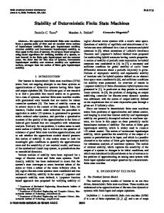
(42) which suggests and , as required in (2). In addition to the examples in Table I, all -stable distributions for (which include Cauchy and Lévy distributions) are -compressible for . C. Realizations of an i.i.d. Sequence We illustrate in Fig. 1, a realization of an i.i.d. sequence with ; decaying like ). In the Student’s distribution ( upper graph, we focus on the first terms, while we show a broader view of the same sequence in the lower graph. We observe that the significant samples in the first 100 terms become insignificant when 1000 terms are considered. In other words, as increases, we observe larger peaks in the sequence, which leads to dramatic changes in the energy of the truncated sequence depending on whether or not these peaks are considered. D. Energy Fraction in Practice To visualize the concept of s-compressibility in i.i.d. sequences, we have plotted the average curves of for Gaussian, Laplace, Cauchy, and Student’s distributions in Fig. 2. We set and averaged the curves over 500 different realizations. Theorem 3 implies that Student’s distribution with is compressible. In Fig. 2, we observe that its energy fraction curve saturates at very small values of . According to Theorem 3, the curve for Student’s distribution will be a step function in the limiting case of . Conversely, Gaussian and Laplace distributions are not compressible in any sense and we expect their asymptotic curves to be close to the ones depicted

5200

IEEE TRANSACTIONS ON SIGNAL PROCESSING, VOL. 59, NO. 11, NOVEMBER 2011

of a sequence can be determined in any domain. However, due to the requirement of independence, the -term approximation of the sequence should be carried out preferentially in the innovation domain. V. CONCLUSION

Fig. 2. Average curve of

with respect to

when

and

for i.i.d. realizations of the Gaussian, Laplace, Cauchy, and Student’s distributions.

In this paper, we first proposed a definition for compressibility of infinite sequences (s-compressibility) that is consistent with the intuition and is mathematically exploitable. We then defined compressibility and sparsity for i.i.d. random sequences. Our definitions are based on the asymptotic distribution of the energy among the elements in truncated subsequences. We showed that some exponentially decaying probability density such as the Laplace distribution are not proper candidates for a s-compressible prior. This arises because they distribute the energy in the sequence rather uniformly. On the other hand, by using order statistics, we demonstrated the connection between the s-compressibility of a heavy-tail distribution and the stability index to which it is attracted. APPENDIX A PROOF OF LEMMA 3 Since Defining

Fig. 3. Average curve of with different sequence lengths distribution are considered.

and

are non-negative, the left inequality is trivial. , we can write that

with respect to for and when i.i.d. realizations of the Cauchy

in Fig. 2. Meanwhile, the fate of the Cauchy distribution is as yet undecided; since it decays like , we know that it is -compressible for ; however, our results are not enough to decide for . E. Effect of

(43) Since is a sum of i.i.d. random variables with unit mean, we have . Thus, is a tail probability. The following approach is a classical method to show the exponential decay of the tail probability:

To investigate the role of in s-compressibility of distributions, we have plotted the average energy fraction curves for Cauchy distribution with and and , where . As predicted by Theorem 3, the curves for approach the step function when increases. The curves for seem to have a continuous limit. F. Linear Transformations It is interesting to mention that, since -stable distributions satisfy a generalized form of the central-limit theorem, they are closed under linear transformations. In other words, the stability index of a stable law does not change whatever the linear-transformation may be. This suggests that the s-compressibility status

(44) where the first inequality is obtained by applying Markov’s inequality.

AMINI et al.: COMPRESSIBILITY OF DETERMINISTIC AND RANDOM INFINITE SEQUENCES

APPENDIX B PROOF OF LEMMA 4 . Since Similarly to the proof of Lemma 3, let s are i.i.d., the probability density function of is found by convolving times the standard exponential distribution with itself:

[12] R. Gribonval, V. Cevher, and M. Davies, “Compressible priors for high-dimensional statistics,” Feb. 2011 [Online]. Available: http://arxiv.org/abs/1102.1249 [13] G. Samorodnitsky and M. S. Taqqu, Stable Non-Gaussian Random Processes. London, U.K.: Chapman & Hall/CRC, 1994. [14] W. Feller, An Introduction to Probability Theory and Its Applications, 2nd ed. New York: Wiley, 1991, vol. 2. [15] R. Lepage, M. Woodroofe, and J. Zinn, “Convergence to a stable distribution via order statistic,” Ann. Probability, vol. 9, no. 4, pp. 624–632, 1981.

(45)

Arash Amini received B.Sc., M.Sc., and Ph.D. degrees in electrical engineering (communications and signal processing) in 2005, 2007, and 2011, respectively, and the B.Sc. degree in petroleum engineering (Reservoir) in 2005, all from Sharif University of Technology (SUT), Tehran, Iran. Since April 2011, he has been a Postdoctoral Researcher in the Biomedical Imaging Group (BIG), École Polytechnique Fédérale de Lausanne, Lausanne, Switzerland. His research interests include different aspects of sampling, specially compressed

Thus, we have that (46) which yields

5201

sensing.

(47)

ACKNOWLEDGMENT The authors would like to thank P. Thévenaz and P. Tafti for their fruitful comments. REFERENCES [1] E. Candes, J. Romberg, and T. Tao, “Robust uncertainty principles: Exact signal reconstruction from highly incomplete frequency information,” IEEE Trans. Inf. Theory, vol. 52, no. 2, pp. 489–509, Feb. 2006. [2] E. Candes and T. Tao, “Near optimal signal recovery from random projections: Universal encoding strategies,” IEEE Trans. Inf. Theory, vol. 52, no. 12, pp. 5406–5425, Dec. 2006. [3] D. Donoho, “Compressed sensing,” IEEE Trans. Inf. Theory, vol. 52, no. 4, pp. 1289–1306, 2006. [4] R. A. DeVore, “Nonlinear approximation,” Acta Numer., vol. 7, pp. 51–150, 1998. [5] E. J. Candes, “Compressive sampling,” in Proc. Int. Congr. Math., 2006, vol. 3, pp. 1433–1452. [6] A. Cohen, W. Dahmen, and R. DeVore, “Compressed sensing and best -term approximation,” J. Amer. Math. Soc., vol. 22, pp. 211–231, 2009. [7] D. P. Wipf and B. D. Rao, “Sparse Baysian learning for basis selection,” IEEE Trans. Signal Process., vol. 52, no. 8, pp. 2153–2164, Aug. 2004. [8] T. Park and G. Casella, “The Bayesian lasso,” J. Amer. Stat. Assoc., vol. 103, pp. 681–686, Jun. 2008. [9] V. Cevher, “Learning with compressible priors,” presented at the Neural Inf. Process. Syst. (NIPS), Vancouver, B.C., Canada, 2008. [10] V. Cevher, “Approximate distributions for compressible signals,” in Proc. IEEE Inf. Theory Workshop, Oct. 2009, p. 353. [11] Y. Zhang, J. Schneider, and A. Dubrawski, “Learning compressible models,” in SIAM Int. Conf. Data Mining, Apr. 2010, pp. 872–881.

Michael Unser (M’89–SM’94–F’99) received the M.S. (summa cum laude) and Ph.D. degrees in electrical engineering from the École Polytechnique Fédérale de Lausanne (EPFL), Switzerland, in 1981 and 1984, respectively. From 1985 to 1997, he worked as a Scientist with the National Institutes of Health, Bethesda, MD. He is currently a Full Professor and Director of the Biomedical Imaging Group at the EPFL. His main research area is biomedical image processing. He has a strong interest in sampling theories, multiresolution algorithms, wavelets, and the use of splines for image processing. He has published 200 journal papers on those topics. Dr. Unser has held the position of Associate Editor-in-Chief for the IEEE TRANSACTIONS ON MEDICAL IMAGING from 2003 to 2005 and has served as Associate Editor for the same journal from 1999 to 2002 and from 2006 to 2007), the IEEE TRANSACTIONS ON IMAGE PROCESSING from 1992 to 1995, and the IEEE SIGNAL PROCESSING LETTERS from 1994 to 1998. He is currently member of the editorial boards of Foundations and Trends in Signal Processing, and Sampling Theory in Signal and Image Processing. He co-organized the first IEEE International Symposium on Biomedical Imaging (ISBI 2002) and was the founding chair of the technical committee of the IEEE-SP Society on Bio Imaging and Signal Processing (BISP). He received the 1995 and 2003 Best Paper Awards, the 2000 Magazine Award, and two IEEE Technical Achievement Awards (2008 SPS and 2010 EMBS). He is an EURASIP Fellow and a member of the Swiss Academy of Engineering Sciences. He is one of ISIs Highly Cited authors in Engineering (http://isihighlycited.com). Farokh Marvasti (S’72–M’74–SM’83) received the B.S., M.S., and Ph.D. degrees all from Rensselaer Polytechnic Institute, Troy, NY, in 1970, 1971, and 1973, respectively. He has worked, consulted, and taught in various industries and academic institutions since 1972, among which are Bell Labs, the University of California Davis, the Illinois Institute of Technology, the University of London, and King’s College. He is currently a Professor at Sharif University of Technology, Tehran, Iran, and the Director of the Advanced Communications Research Institute (ACRI) and head of the Center for Multi-Access Communications Systems. He has about 100 journal publications and has written several reference books, his last book being Nonuniform Sampling: Theory and Practice (Kluwer, 2001). He also has several international patents. Dr. Marvasti was one of the editors and associate editors of the IEEE TRANSACTIONS ON COMMUNICATIONS and the TRANSACTIONS ON SIGNAL PROCESSING from 1990 to 1997. He was also a Guest Editor on the May 2008 Special Issue on Nonuniform Sampling for the Sampling Theory & Signal and Image Processing journal. Besides being the co-founder of two international conferences (ICTs and SampTAs), he has been the organizer and special session chair of many IEEEE conferences, including ICASSP conferences.