3914
IEEE TRANSACTIONS ON SIGNAL PROCESSING, VOL. 63, NO. 15, AUGUST 1, 2015
Hybrid Random/Deterministic Parallel Algorithms for Convex and Nonconvex Big Data Optimization Amir Daneshmand, Francisco Facchinei, Vyacheslav Kungurtsev, and Gesualdo Scutari, Senior Member, IEEE
Abstract—We propose a decomposition framework for the parallel optimization of the sum of a differentiable (possibly nonconvex) function and a nonsmooth (possibly nonseparable), convex one. The latter term is usually employed to enforce structure in the solution, typically sparsity. The main contribution of this work is a novel parallel, hybrid random/deterministic decomposition scheme wherein, at each iteration, a subset of (block) variables is updated at the same time by minimizing a convex surrogate of the original nonconvex function. To tackle huge-scale problems, the (block) variables to be updated are chosen according to a mixed random and deterministic procedure, which captures the advantages of both pure deterministic and random update-based schemes. Almost sure convergence of the proposed scheme is established. Numerical results show that on huge-scale problems the proposed hybrid random/deterministic algorithm compares favorably to random and deterministic schemes on both convex and nonconvex problems. Index Terms—Jacobi method, nonconvex problems, parallel and distributed methods, random selections, sparse solution.
I. INTRODUCTION ECENT years have witnessed a surge of interest in very large scale optimization problems, and the evocative term Big Data optimization has been coined to denote this new area of research. Many such problems can be formulated as the minimization of the sum of a smooth (possibly nonconvex) function and of a nonsmooth (possibly nonseparable) convex one :
R
(1)
Manuscript received September 02, 2014; revised February 11, 2015 and May 03, 2015; accepted May 05, 2015. Date of publication June 01, 2015; date of current version June 17, 2015. The associate editor coordinating the review of this manuscript and approving it for publication was Prof. Ami Wiesel. The work of Daneshmand and Scutari was supported by the USA NSF Grants CMS 1218717 and CAREER Award No. 1254739. The work of Facchinei was supported by the MIUR project PLATINO (Grant Agreement n. PON01_01007). The work of Kungurtsev was supported by the European Social Fund unde.r the Grant CZ.1.07/2.3.00/30.0034. Part of this work has been presented at the Asilomar Conference2014 [1]. The order of the authors in the byline is alphabetical as each author contributed equally. A Daneshmand is with the Department of Electrical Engineering, State University of New York at Buffalo, Buffalo 14228 USA (e-mail:
[email protected]). F. Facchinei is with the Department of Computer, Control, and Management Engneering, University of Rome La Sapienza, Rome 00185, Italy (e-mail:
[email protected]). V. Kungurtsev is with the Agent Technology Center, Department of Computer Science, Faculty of Electrical Engineering, Czech Technical University, Prague 166 36, Czech Republic (e-mail:
[email protected]). G. Scutari is with the School of Industrial Engineering, Purdue University, West Lafayette, IN 47907 USA (e-mail:
[email protected]). Color versions of one or more of the figures in this paper are available online at http://ieeexplore.ieee.org. Digital Object Identifier 10.1109/TSP.2015.2436357
where is a closed convex set with a cartesian product structure: . Our focus is on problems with a huge number of variables, as those that can be encountered, e.g., in machine learning, compressed sensing, data mining, tensor factorization and completion, network optimization, image processing, genomics, etc.. We refer the reader to [2]–[14] and the books [15], [16] as entry points to the literature. Block Coordinate Descent (BCD) methods rapidly emerged as a winning paradigm to attack Big Data optimization, mainly due to their low-cost per-iteration and scalability; see e.g. [4]. At each iteration of a BCD method one block of variables is updated using first-order information, while keeping all other variables fixed. Several choices of the block of variables to update at each iteration have been studied, including cyclic orders and greedy/opportunistic selection strategies, the latter aiming to select the block leading to the largest decrease of the objective function. The cyclic order has the advantage of being extremely simple, but the greedy strategy usually provides faster convergence, at the cost of an increased computational effort at each iteration. However, no matter which block selection rule is adopted, as the dimensions of the optimization problems increase, even BCD methods may result inadequate. To alleviate the “curse of dimensionality”, three different kind of strategies have been proposed, namely: (a) parallelism, where several blocks of variables are updated simultaneously in a multicore or distributed computing environment, see e.g. [6]–[8], [8]–[11], [17]–[26]; (b) random selection of the block(s) of variables to update, see e.g. [21]–[31]; and (c) use of “more-thanfirst-order” information, for example (approximated) Hessians or (parts of) the original function itself, see e.g. [5], [19], [20], [32], [33]. Point (a) is self-explanatory and rather intuitive; here we only remark that the vast majority of parallel BCD methods apply to convex problems only. Points (b) and (c) need further comments. Point (b): Random selection-based rules are essentially as cheap as cyclic selections while alleviating some of the pitfalls of cyclic updates. They are also relevant in distributed environments wherein data are not available in their entirety, but are acquired either in batches or over a network. In such scenarios, one might be interested in running the optimization at a certain instant even with the limited, randomly available information. The main limitation of random selection rules is that they remain disconnected from the status of the optimization process, which instead is exactly the kind of behavior that greedy-based updates try to avoid, in favor of faster convergence, but at the cost of more intensive computation. Point (c): The use of “more-than-first-order” information also has to do with the trade-off between cost-per-iteration and overall cost of the optimization process. Although using higher order or structural information may seem unreasonable in Big
1053-587X © 2015 EU
DANESHMAND et al.: HYBRID RANDOM/DETERMINISTIC PARALLEL ALGORITHMS
Data problems, recent studies, as those mentioned above, suggest that a judicious use of some kind of “more-than-first-order” information can lead to substantial improvements. The above pros & cons analysis suggests that it would be desirable to design a parallel algorithm for nonconvex problems combining the benefits of random sketching and greedy updates, possibly using “more-than-first-order” information. To the best of our knowledge, no such algorithm exists in the literature. In this paper, building on our previous deterministic methods [19], [20], [34], we propose a BCD-like scheme for the computation of stationary solutions of Problem (1) filling the gap and enjoying all the following features: 1) It uses a random selection rule for the blocks, followed by a deterministic subselection; 2) It can classically tackle separable convex function , i.e., , but also nonseparable functions ; 3) It can deal with a nonconvex functions ; 4) It can use both first-order and higher-order information; 5) It is parallel; 6) It can use inexact updates; 7) It converges almost surely, i.e., our convergence results are of the form “with probability one”. As far as we are aware of, this is the first algorithm enjoying all these properties, even in the convex case. The combination of features 1–7 in one single algorithm is a major achievement in itself, which offers great flexibility to develop tailored convergent solutions methods within the same framework. Last but not least, our experiments show impressive performance of the proposed methods, outperforming state-of-the-art solution scheme (cf. Section IV). As a final remark, we underline that, at more methodological level, the combination of all features 1–7 and, in particular, the need to conciliate random and deterministic strategies, led to the development of a new type of convergence analysis (see Appendix A) which is also of interest per se and could bring to further developments. Below we further comment on some of features 1–7, compare to existing results, and detail our contributions. Feature 1: The idea of making a random selection and then perform a greedy subselection has been previously discussed only in [35]. However, results therein i) are only for convex problems with a specific structure; ii) are based on a regularized first-order model; iii) require a very stringent “spectral-radius-type” condition to guarantee convergence, which severely limits the degree of parallelism; and iv) convergence results are in terms of expected value of the objective function. The proposed algorithmic framework expands vastly on this setting, while enjoying also all properties 2–7. In particular, it is the first hybrid random/greedy scheme for nonconvex nonseparable functions, and it allows any degree of parallelism (i.e., the update of any number of variables); and all this is achieved under much weaker convergence conditions than those in [35], satisfied by most of practical problems. Numerical results show that the proposed hybrid schemes is very effective, and seems to preserve the advantages of both random and deterministic selection rules, see Section IV. Feature 2: The ability of dealing with some classes of nonseparable convex functions has been documented in [36]–[38], but only for deterministic and sequential schemes; our approach extends also to parallel, random schemes. Feature 3: The list of works dealing with BCD methods
3915
for nonconvex ’s is short: [23], [30] for random sequential methods; and [8], [18], [19], [20] for deterministic parallel ones. Random (and cyclic) parallel methods for nonconvex ’s are studied, independently from this work but drawing on our results [19] and [20], also in [39]. The present paper has several distinct significant contributions above and beyond [39], namely: i) the use, for the first time in the field, of a hybrid parallel-greedy update scheme (Feature 1); ii) the first parallel scheme with some convergence guarantees for nonseparable regularizers (Feature 2); iii) the use of inexact updates, which for huge scale problems can be an essential property (Feature 6); and iv) an entirely new proof technique for random updates introduced to the literature. Numerical results in Section IV show that the additional features we provide, in particular Feature 1, are fundamental for a good numerical behavior: it will be seen that using a hybrid greedy-random scheme tends to consistently result in faster convergence than the purely random one discussed in [39]. Dual ADMM-like schemes have been proposed for problems with a specific nonconvex, additively separable , and shown to be convergent under strong conditions; see, e.g., [40]. However, for the scale and generality of problems we are interested in, they are computationally impractical. Feature 4: We want to stress the ability of the proposed algorithm to exploit in a systematic way “more-than-first-order” information. Differently from BCD methods that use at each iteration a (possibly regularized) first-order model of the objective function, our method provides the flexibility of using more sophisticated models, including Newton-like surrogates as well as more structured functions as those described in the following example. Suppose that in (1) , where is convex and is not. Then, at iteration , one could base the update of the -th block on the surrogate function , where denotes the vector obtained from by deleting . The rationale here is that instead of linearizing the whole function we only linearize the difficult, nonconvex part . In this light we can also better appreciate the importance of feature 6, since if we go for more complex surrogate functions, the ability to deal with inexact solutions becomes important. Feature 6: Inexact solution methods have been little studied. Papers [4], [41], [42] (somewhat indirectly) consider some of these issues for -loss linear support vector machines problems. A more systematic treatment of inexactness of the solution of a first-order model is documented in [43], in the context of random sequential BCD methods for convex problems. Our results in this paper are based on our previous works [19], [20], [34], where both the use of “more-than-first-order” models and inexactness are introduced and rigorously analyzed in the context of parallel, deterministic methods. A further contribution of the paper is extensive testing of our schemes and the most competitive deterministic and random ones in the literature on a parallel architecture. More specifically, tests were carried out on i) LASSO problems, one of the most studied convex instance of Problem (1); and two nonconvex problems, namely: ii) a nonconvex modification of LASSO; and iii) dictionary learning problems. In the experiments on LASSO, we compared our scheme with: PCDM and PCDM2 [26]; Hydra [44] and [21]; FLEXA [19], [20]; and the random algorithm in [39]. For the nonconvex problem
3916
IEEE TRANSACTIONS ON SIGNAL PROCESSING, VOL. 63, NO. 15, AUGUST 1, 2015
ii) we contrasted our scheme with: FLEXA, SpaRSA [10], FISTA [9] (FISTA does not have any convergence guarantee but nevertheless we included it to the comparison because of its benchmark status in the convex case), and the random algorithm in [39]. For dictionary learning problem, we also added the ad-hoc method proposed in [45]. The paper is organized as follows. Section II formally introduces the optimization problem along with several motivating examples and also discusses some technical points. The proposed algorithmic framework and its convergence properties are introduced in Section III, while numerical results are presented in Section IV. Section V draws some conclusions. II. PROBLEM DEFINITION AND PRELIMINARIES A. Problem definition We consider Problem (1), where the feasible set is a Cartesian product of lower dimensional convex sets , and is partitioned accordingly: , with each ; we denote by the set of the blocks. The function is smooth (and not necessarily convex and separable) and is convex, and possibly nondifferentiable and nonseparable. Problem (1) is very general and includes many popular Big Data formulations; some examples are listed next. Ex. #1-(group) LASSO: and (or , ), , with , , and given constants; (group) LASSO has long been used in many applications in signal processing and statistics [2]. Ex. #2-linear regression: and , , with , and given constants; the norm linear regression is widely used techniques in statistics [46]. Note that is nonseparable. Ex. #3-The Fermat-Weber problem: and , , with , , and given constants, for all ; this problem, such that the weighted sum which consists in finding of distances between and the anchors , was widely investigated in the optimization as well as location communities; see, e.g., [47]. This is another example of nonseparable . Ex. #4-The TV image reconstruction: and , , where , , , , and is the discrete total variational or 2 and being the discrete semi-norm of , with defined as , gradient of if and with otherwise, and if and otherwise [48]. This is the well-known noise-free discrete TV model for compressing sensing image reconstruction [48]; TV minimizing models have become a successful methodology for image processing, including denoising, deconvolution, and restoration, to name a few. Ex. #5-Dictionary learning: and , , where and are the (matrix) optimization variables, , , are given constants, is the -dimensional and
vector with a 1 in the -th coordinate and 0’s elsewhere, and and denote the Frobenius norm and the matrix norm of , respectively; this is an example of the dictionary learning problem for sparse representation [49] that finds numerous applications in various fields such as computer vision and signal and image processing. Note that is not jointly convex in Ex. #6-Matrix completion: , , , where is a given subset of . Matrix completion has found numerous applications in various fields such as recommender systems, computer vision, and system identification. Other problems of interest that can be cast in the form (1) include the Logistic Regression, the Support Vector Machine, the Nuclear Norm Minimization, the Robust Principal Component Analysis, the Sparse Inverse Covariance Selection, and the Nonnegative Tensor Factorization; see, e.g., [50]. Assumptions: Given (1), we make the following blanket assumptions: (A1) Each is nonempty, closed, and convex; (A2) is on an open set containing ; is Lipschitz continuous on with constant ; (A3) (A4) is continuous and convex on (possibly nondifferentiable and nonseparable); (A5) is coercive, i.e., . The above assumptions are standard and are satisfied by many practical problems. For instance, A3 holds automatically if is bounded, whereas A5 guarantees the existence of a solution. With the advances of multi-core architectures, it is desirable to develop parallel solution methods for Problem (1) whereby operations can be carried out on some or (possibly) all (block) variables at the same time. The most natural parallel (Jacobi-type) method one can think of is updating all blocks simultaneously: given , each (block) variable is updated by solving the following subproblem (2) Unfortunately this method converges only under very restrictive conditions [51] that are seldom verified in practice (even in the absence of the nonsmooth part ). Furthermore, the exact computation of may be difficult and computationally too expensive. To cope with these issues, a natural approach is to replace the (nonconvex) function by a suitably chosen local convex surrogate , and solve instead the convex problems (one for each block)
(3) with the understanding that the minimization in (3) is simpler than that in (2). Note that the function has not been touched; this is because i) it is generally much more difficult to find a “good” surrogate of a nondifferentiable function than of a differentiable one; ii) is already convex; and iii) the functions encountered in practice do not make the optimization problem (3) difficult (a closed form solution is available for a large classes of ’s, if are properly chosen). In this work we assume that , have the folthe surrogate functions lowing properties:
DANESHMAND et al.: HYBRID RANDOM/DETERMINISTIC PARALLEL ALGORITHMS
(F1) on ; (F2) (F3)
is uniformly strongly convex with constant for all ; is Lipschitz continuous on for all
;
is the partial gradient of with respect to (w.r.t.) where its first argument . Function should be regarded as a (simple) convex surrogate of at the point w.r.t. the block of variables that preserves the first order properties of w.r.t. . Note that, contrary to most of the works in the literature (e.g., [38]), we do not require to be a global upper surrogate of , which significantly enlarges the range of applicability of the proposed solution methods. The most popular choice for satisfying F1–F3 is
(4) with . This is essentially the way a new iteration is computed in most (block-)BCDs for the solution of LASSO problems and its generalizations. When , this choice gives rise simply by a to a gradient-type scheme; in fact we obtain shift along the antigradient. As we discussed in Section I, this is a first-order method, so it seems advisable, at least in some situations, to use more informative -s. If is convex, an alternative is to take as a second order expansion of around , i.e.,
(5) where is nonnegative and can be taken to be zero if is actually strongly convex. When , this essentially corresponds to taking a Newton step in minimizing the “reduced” problem . Still in the case of a , one could also take uniformly strongly convex just , which preserves the structure of the function. Other valuable choices tailored to specific applications are discussed in [20], [34]. As a guideline, note that our method, as we shall describe in details shortly, is based on the iterative (approximate) solution of problem (3) and therefore a balance should be aimed at between the accuracy of the surrogate and the ease of solution of (3). Needless to say, the option (4) is the less informative one, but usually it makes the computation of the solution of (3) a cheap task. Best-response map: Associated with each and , under F1-F3, one can define the following block solution map: (6) is always well-defined, since the optimization Note that problem in (6) is strongly convex. Given (6), we can then introduce the solution map (7) Our algorithmic framework is based on solving in parallel a suitable selection of subproblems (6), converging thus to fixed-
3917
points of (of course the selection varies at each iteration). It is then natural to ask which relation exists between these fixed points and the stationary solutions of Problem (1). To answer this key question, we recall first two basic definitions. Stationarity: A point is a stationary point of (1) if a subgraexists such that dient for all . Coordinate-wise stationarity: A point is a coordinate-wise , with stationary point of (1) if subgradients , exist such that , for all and . In words, a coordinate-wise stationary solution is a point for which is stationary w.r.t. every block of variables. Coordinate-wise stationarity is a weaker form of stationarity. It is the standard property of a limit point of a convergent coordinate-wise scheme (see, for example [36]–[38]). It is clear that a stationary point is always a coordinate-wise stationary point; the converse however is not always true, unless extra conditions on are satisfied. Regularity: Problem (1) is regular at a coordinate-wise stationary point if is also a stationary point of the problem. The following two cases imply the regularity condition, (a) is separable (still nonsmooth), i.e., ; (b) is continuously differentiable around . , whereas (b) folNote that (a) is due to lows from . Of course these two cases are not at all inclusive of situations for which regularity holds. As an example of a nonseparable function for which regularity holds at a point at which is not continuously differentiable, consider the function arising in logistic regression problems , with , and and being given ; the resulting function constants. Now, choose is continuously differentiable, and therefore regular, at any stationary point but . It is easy to verify that is also , if . regular at The algorithm we present in the paper expands upon the literature in presenting the first (deterministic or random) parallel coordinate-wise scheme that converges to coordinate-wise stationary points. Under the regularity condition these points are also stationary, and so among the class of parallel algorithms, the method we present enlarges the class of problems for which convergence to stationary points is achieved for Problem (1) to include some classes of nonseparable . Certainly, proximal gradient-like algorithms can converge to stationary points for any nonseparable , but such schemes are inherently incapable of parallelization, and thus are typically much slower in practice. Thus, our algorithm is a step towards, if not complete fulfillment of, the desiderata of a parallel algorithm that converges to stationary points for all classes of Problem (1) with arbitrary nonsmooth convex . The following proposition is elementary and elucidates the connections between stationarity conditions of Problem (1) and fixed-points of . Proposition 1: Given Problem (1) under A1–A5 and F1–F3, the following hold: i) The set of fixed-points of coincides with the coordinatewise stationary points of Problem (1); ii) If, in addition, Problem (1) is regular at a fixed-point of , then such a fixed-point is also a stationary point of the problem.
3918
IEEE TRANSACTIONS ON SIGNAL PROCESSING, VOL. 63, NO. 15, AUGUST 1, 2015
III. ALGORITHMIC FRAMEWORK We begin introducing a formal description of the salient characteristic of the proposed algorithmic framework—the novel hybrid random/greedy block selection rule. The random block selection works as follows: at each iteration , a random set is generated, and the blocks are the potential candidate variables to update in parallel. The set is a realization of a random set-valued mapping with values in the power set of . We do not constraint to any specific distribution; we only require that, at each iteration , each block has a positive probability (possibly nonuniform) to be selected. (A6) The sets are realizations of independent random setsuch that , for all valued mappings and , and some . A random selection rule satisfying A6 will be called proper sampling. Several proper sampling rules will be discussed in details shortly. The proposed hybrid random/greedy block selection rule consists in combining random and greedy updates in the following form. First, a random selection is performed—the set is generated. Second, a greedy procedure is run to select in the pool only the subset of blocks, say , that are “promising” (according to a prescribed criterion). Finally all the blocks in are updated in parallel. The notion of “promising” block is made formal next. Since is an optimal solution of (6) if and only if , a natural distance of from the optimality is . The blocks in to be updated can be then chosen based on such an optimality measure (e.g., opting for blocks exhibiting larger ’s). Note that in some applications, including some of those discussed in Section II, given a proper block decomposition, can be computed easily in closed form, see Section IV for three different examples. However, this is not always the case, and on some problems, the computation of might be too expensive. In these cases it might be useful to introduce alternative, less expensive metrics by replacing the distance with a computationally cheaper error bound, i.e., a function such that (8) . We refer the interested reader to [20] for some for some more details, and to [52] as an entry point to the vast literature on error bounds. As an example, if problem (1) is unconstrained, , and we are using the surrogate function given by (4), a suitable error bound is the function with and . The proposed hybrid random/greedy scheme capturing all the features 1)–6) discussed in Section I is formally given in Algorithm 1. Note that in step S.3 inexact calculations of are allowed, which is another noticeable and useful feature: one can reduce the cost per iteration without affecting too much, experience shows, the empirical convergence speed. In step S.5 we introduced a memory in the variable updates: the new point is a convex combination via of and . The convergence properties of Algorithm 1 are given next. Theorem 2: Let be the sequence generated by Algorithm 1, under A1–A6. Suppose that and
Algorithm 1: Hybrid Random/Deterministic Flexible Parallel Algorithm (HyFLEXA) Data:
for
,
,
.
.
Set (S.1): If
,
satisfies a termination criterion: STOP;
(S.2): Randomly generate a set of blocks (S.3): Set
. that contains at least one .
Choose a subset index for which (S.4): For all s.t. Set
for
, solve (6) with accuracy ; and
(S.5): Set (S.6):
: find
for ;
, and go to (S.1).
satisfy the following conditions: i) ; ii) ; iii) ; iv) ; and v) for all and some nonnegative constants and . Additionally, if inexact solutions are used in Step 3, i.e., for some and infinite , then assume also that is globally Lipschitz on . Then, either Algorithm 1 converges in a finite number of iterations to a fixed-point of of (1) or there exists at least one limit point of that w.p.1. is a fixed-point of Proof: See Appendix C. Remark 3: Note that the conditions on imply that for all . The Theorem provides minimal conditions under which convergence can be guaranteed. Practically, of course the choice of will affect the practical performance of the algorithm and the appropriate choice is problem dependent and given by practical experience. The convergence results in Theorem 2 can be strengthened when is separable. Theorem 4: In the setting of Theorem 2, suppose in addition that is separable, i.e., . Then, either Algorithm 1 converges in a finite number of iterations to a stationary solution of Problem (1) or every limit point of is a stationary solution of Problem (1) w.p.1. Proof: See Appendix D. On the Random Choice of : We discuss next some proper sampling rules that can be used in Step 3 of the algorithm to generate the random sets ; for notational simplicity the iteration index will be omitted. The sampling rule is uniquely characterized by the probability mass function
which assign probabilities to the subsets of . Associated , for with , define the probabilities . The following proper sampling rules, proposed in [26] for convex problems with separable , are instances of
DANESHMAND et al.: HYBRID RANDOM/DETERMINISTIC PARALLEL ALGORITHMS
rules satisfying A6, and are used in our computational experiments. — Uniform (U) sampling. All blocks get selected with the same (non zero) probability:
— Doubly Uniform (DU) sampling. All sets of equal cardinality are generated with equal probability, i.e., , such that . The density function is for all then
— Nonoverlapping Uniform (NU) sampling. It is a uniform sampling assigning positive probabilities only to sets forming a partition of . Let be a partition of , with each , the density function of the NU sampling is: if otherwise which corresponds to , for all . A special case of the DU sampling that we found very effective in our experiments is the so called “nice sampling”. — Nice Sampling (NS). Given an integer , a -nice sampling is a DU sampling with (i.e., each subset of blocks is chosen with the same probability). The NS allows us to control the degree of parallelism of the algorithm by tuning the cardinality of the random sets generated at each iteration, which makes this rule particularly appealing in a multi-core environment. Indeed, one can set equal to the number of available cores/processors, and assign each block coming out from the greedy selection (if implemented) to a dedicated processor/core. As a final remark, note that the DU/NU rules contain as special cases fully parallel and sequential updates, wherein at each iteration a single block is updated uniformly at random, or all blocks are updated. — Sequential sampling: It is a DU sampling with , or a and , for . NU sampling with — Fully parallel sampling: It is a DU sampling with , or a NU sampling with and . Other interesting uniform and nonuniform practical rules (still satisfying A6) can be found in [26], [53]. In addition see [54] for extensive numerical results comparing the different sampling schemes. On the Choice of the Step-Size : An example of step-size rule satisfying Theorem 2i)-iv) is: given , let (9) is a given constant. Numerical results in where Section IV show the effectiveness of (9) on specific problems. We remark that it is possible to prove convergence of Algorithm 1 also using other step-size rules, including a standard Armijo-like line-search procedure or a (suitably small) constant step-size. Note that differently from most of the schemes in the literature, the tuning of the step-size does not require the knowledge of the problem parameters (e.g., the Lipschitz constants of and ).
3919
IV. NUMERICAL RESULTS In this section we present some preliminary experiments providing solid evidence of the viability of our approach. Tests were carried out on i) LASSO problems, one of the most studied (convex) instances of Problem (1); and two nonconvex problems, namely: ii) a nonconvex modification of LASSO, and iii) dictionary learning problems. A complete assessment of the numerical behavior of our method is beyond the scope of this paper, since it would require very extensive experiments, especially for nonconvex problems, where comparisons of methods should take into account the existence of multiple stationary points with (possibly) different objective values and a strong influence of the starting points. Furthermore we remark that a proper comparison should be made only with other random, parallel methods for nonconvex problems. However, Algorithm 1 appears to be the first of this kind, together with the very recent proposal in [39] (which is a special case of Algorithm 1). Therefore, while in the convex case we could compare to some well-established methods, in the nonconvex case we could only compare to [39]. In order to enlarge the pool of comparisons, and also to give a better perspective on our approach, we decide to include in the comparisons also deterministic methods. Of course, one should always keep in mind that deterministic and random BCD methods have different purposes. Random BCD algorithms are the methods of choice when it is not possible to process all data at the same time, either because the data become available at different times (for example in a network with propagation delays) or, simply, because the dimensions of the problem are so huge that the use of deterministic methods, requiring access to all variables at each iteration, is not practically possible. In spite of all caveats above, the tests convincingly show that our framework leads to practical methods that exploit well parallelism and compare favorably to existing schemes, both deterministic and random. It should be remarked that i) our method, designed to handle also nonconvex problems, seems to perform well also when compared to schemes specifically designed for convex problems only, and ii) in some cases, it outperforms even the most efficient deterministic methods, a result that is somewhat surprising, given the different amount of information required by deterministic methods. All codes have been written in C++ and use the Message Passing Interface for parallel operations. All algebra is performed by using the Intel Math Kernel Library (MKL). The algorithms were tested on the General Compute Cluster of the Center for Computational Research at the SUNY Buffalo. In particular for our experiments we used a partition composed of 372 DELL 32 2.13 GHz Intel E7-4830 Xeon Processor nodes with 512 GB of DDR4 main memory and QDR InfiniBand 40 Gb/s network card. A. LASSO Problems Lasso problems were described in Section II, here we report the results obtained on a set of randomly generated problems. Tuning of Algorithm 1: The most successful class of random and deterministic methods for LASSO problem are (proximal) gradient-like schemes, based on a linearization of . As a major departure from current schemes, here we propose to better exploit the structure of and use in Algorithm 1 the following
3920
IEEE TRANSACTIONS ON SIGNAL PROCESSING, VOL. 63, NO. 15, AUGUST 1, 2015
best-response: given a scalar partition of the variables (i.e., for all ), let
(10) Note that has a closed form expression (using a softthresholding operator [9]). The free parameters of Algorithm 1 are chosen as follows. The proximal gains and the step-size are tuned as in [20, Sec. VI.A]. The error bound function is chosen as , and, for any realiza, the subsets in S.3 of the algorithm are chosen as tion . We denote by the cardinality of normalized to the overall number of variables; in our experiments, all sets are generated using the NU sam, for all . We report results for the folpling, with lowing values of and : i) ; ii) , which leads to a fully parallel pure random scheme are updated; and wherein at each iteration all variables in iii) different positive values of ranging from 0.01 to 0.5, which corresponds to updating in a greedy manner only a subset of the “Random variables in . We termed Algorithm 1 with FLEXible parallel Algorithm” (RFLEXA), whereas the other instances with as “Hybrid FLEXA” (HyFLEXA). We note that RFLEXA should be regarded both as a particular instance of our scheme and as an efficient implementation of the method proposed in [39], with many nontrivial algorithmic choices made according to our experience in [20] in order to optimize its behavior. As we remarked before, RFLEXA is the only other random, parallel BCD method for which convergence to stationary points of nonconvex problems has been shown. From another perspective, the comparison between HyFLEXA and RFLEXA also serves to gauge the importance of performing a deterministic, greedy block selection after the random one, this being one of the key new ideas of HyFLEXA. Algorithms in the Literature: We compared our versions of (Hy)FLEXA with the most representative parallel random and deterministic algorithms proposed to solve LASSO Problems. More specifically, we consider the following schemes. • PCDM & PCDM2: These are (proximal) gradient-like parallel randomized BCD methods proposed in [26] for convex optimization problems. As recommended by the authors, we use PCDM instead of PCDM2 (indeed, our experiments show that PCDM outperforms PCDM2). We set the parameters and of PCDM as in [26, Table 4], which guarantees convergence of the algorithm in expected value. • Hydra & Hydra : Hydra is a parallel and distributed random gradient-like CDM, proposed in [44]; a closed form solution of the scalar updates is available. Hydra [21] is the accelerated version of Hydra; indeed, in all our experiments, it outperformed Hydra; therefore, we will report the results only for Hydra . The free parameter is set to (cf. Eq. (15) in [44]), with given by Eq. (12) in [44] (according to the authors, this seems one of the best choices for ). • FLEXA: This is the parallel deterministic scheme we proposed in [19], [20]. We use FLEXA as a benchmark of deterministic algorithms, since it has been shown in [19], [20] that for selected test problems, it numerically outperforms current (parallel) first-order (accelerated) gradient-like schemes, including FISTA [9], SparRSA [10], GRock [11], parallel BCD [8], and ADMM. The free parameters of FLEXA, and , are tuned as
Fig. 1. HyFLEXA for different values of and : Relative error vs. time; , 2%, 5%, , 100.000 variables, NU sampling, 8 cores; , and , 0.5—(b) , and , 0.2, 0.5. (a)
in [20, Sec. VI.A], whereas the set is chosen as . • Other algorithms: We tested also other random algorithms, including sequential random BCD-like methods and Shotgun [17]. However, since they were not competitive, to not overcrowd the figures, we do not report results for these algorithms. In all the experiments, the data matrix of the LASSO problem is stored in a column-block manner, uniformly across the parallel processes. Thus the computation (required to evaluate ) and the norm of each product (that is ) is divided into the parallel jobs of computing and , followed by a reduce operation. Also, for all the algorithms, the initial point was set to the zero vector. Numerical Tests: We generated synthetic LASSO problems using the random generation technique proposed by Nesterov [7], which we properly modified following [26] to generate instances of the problem with different levels of sparsity of the solution as well as density of the data matrix ; we introduce the following two control parameters: average % of nonzeros in each column of (out of ); and of nonzeros in the solution (out of ). We tested the algorithms on two groups of LASSO problems, and , and several degrees of density of and sparsity of the solution, namely , 1%, 5%, 15%, 30%, and , 30%, 50%, 70%, 90%. Because of the space limitation, we report next only the most representative results; we refer to [54] for more details and experiments. Results for the LASSO instance with 100,000 variables are reported in Fig. 1 and 2. Fig. 1 shows the behavior of HyFLEXA as a function of the design parameters and , for different values of the solution sparsity ( , whereas in Fig. 2 we compare the proposed RFLEXA and HyFLEXA with FLEXA, PCDM, and Hydra , for different values of and Finally, in Fig. 3 we consider larger problems with 1M variables. In all the figures, we plot the relative error versus the CPU time, where is the optimal value of the is known). All the objective function (in our experiments curves are averaged over ten independent random realizations. Note that the CPU time includes communication times and the initial time needed by the methods to perform all pre-iterations computations (this explains why the curves associated with Hydra start after the others; in fact Hydra requires some nontrivial computations to estimates ). HyFLEXA: On the choice of , and the sampling strategy:
DANESHMAND et al.: HYBRID RANDOM/DETERMINISTIC PARALLEL ALGORITHMS
Fig. 2. LASSO with 100.000 variables, 8 cores; Relative error vs. time for: (a1) and —(a2) and —(b1) and —(b2) and —(c1) and —(c2) and .
Fig. 3. LASSO with 1M variables, —(b) time for: (a)
, 16 cores; Relative error vs. . The legend is as in Fig. 2.
3921
All the experiments (including those not reported here because of lack of space) show the following trend in the behavior of HyFLEXA as a function of . For “low” density problems (“low” and ), “large” pairs are preferable, which corresponds to updating at each iteration only some variables by performing a (heavy) greedy search over a sizable amount of variables. This is in agreement with [20] (cf. Remark 5): by the greedy selection, Algorithm 1 is able to identify those variables that will be zero at the a solution; therefore updating only variables that we have “strong” reason to believe will not be zero at a solution is a better strategy than updating them all, especially if the solutions are very sparse. Note that this behavior can be obtained using either “large” or “small” . However, in the case of “low” dense problems, the former strategy outperforms the latter. We observed that this is mainly due to the fact that when is “small”, estimating (computing the products ) is computationally affordable, and thus performing a greedy search over more variables enhances the practical convergence. When the sparsity of the increases (“large” solution decreases and/or the density of and/or ), one can see from the figures that “smaller” values of are more effective than larger ones, which corresponds to using a “less aggressive” greedy selection while searching over a smaller pool of variables. In fact, when is dense, computing all might be prohibitive and thus nullify the potential benefits of a greedy procedure. For instance, it follows from Fig. 1–3 that, as the density of the solution ( ) increases the preferable choice for progressively moves and decreasing. from (0.5, 0.5) to (0.2, 0.01), with both Interesting, a tuning that works quite well in practice for all the classes of problems we simulated (different densities of , , solution sparsity, number of cores, etc.) is which seems to strike a good balance between not updating variables that are probably zero at the optimum and nevertheless update a sizable amount of variables when needed in order to enhance convergence.. As a final remark, we report that, according to our experiments, the most effective sampling rule among U, DU, NU, and NS is the NU (which is actually the one the figures refers to); NS becomes competitive only when the solutions are very sparse, see [54] for a detailed comparison of the different rules. Comparison of the algorithms: For low dense matrices and very sparse solutions, FLEXA is faster than its random counterparts (RFLEXA and HyFLEXA) as well as its fully parallel version, FLEXA [see Fig. 2 a1), b1) c1) and Fig. 3a)]. Nevertheless, HyFLEXA [with and/or the size remains close. However, as the density of of the problem increase, computing all the products (required to estimate ) becomes too costly; this is when a random selection of the variables becomes beneficial: indeed, RFLEXA and HyFLEXA consistently outperform FLEXA [see Fig. 2 a2), b2) c2) and Fig. 3b)]. Among the random algorithms, Hydra is capable to approach relatively fast low accuracy, especially when the solution is not too sparse, but has difficulties in reaching high accuracy. RFLEXA and HyFLEXA are always much faster than current state-of-the-art schemes (PCDM and Hydra ), especially if high accuracy of the solutions is required. Between RFLEXA and HyFLEXA (with the same ), the latter consistently outperforms the former (about up to five time faster), with a gap that is more significant when solutions are
3922
IEEE TRANSACTIONS ON SIGNAL PROCESSING, VOL. 63, NO. 15, AUGUST 1, 2015
Fig. 4. Nonconvex Quadratic Problem, 50 cores; objective function value vs. time for: (a)
sparse. This provides a solid evidence of the effectiveness of the proposed hybrid random/greedy selection method. B. Nonconvex Quadratic Problems The first set of nonconvex problems we test is a modification of the LASSO problem, as first proposed in [20]. More precisely, we consider the following nonconvex quadratic problems
(11) is no where is a positive constant chosen so that longer convex. We considered two instances of (11), namely: 1) is generated using Nesterov’s model (as in LASSO problems in Section IV-A) with and , , , and ; and 2) the and . Note that same setting as in 1) but with the Hessian of has the same eigenvalues of the Hessian of in the original LASSO problem, but translated in our problem has (many) to the left by . In particular, negative eigenvalues; therefore, the objective function in (11) is (markedly) nonconvex. Since is now unbounded from below by construction, we added in (11) box constraints. Comparison of the Algorithms: We compared HyFLEXA with FISTA, SpaRSA, RFLEXA, and (deterministic) FLEXA. The tuning of FLEXA, RFLEXA, and HyFLEXA is the same as the one used for LASSO problems (cf. Section IV-A), but adding the extra condition , for all , so that the resulting one dimensional subproblems (6) are convex and can be solved in closed form. Note that as far as we are aware of the only parallel random method with convergence guarantees on nonconvex problems is RFLEXA. We therefore report also results for SpaRSA and FLEXA for comparison sake. FISTA does not have any convergence guarantee for nonconvex problems but nevertheless we also added FISTA to the comparison because of its benchmark status in the convex case. On our tests, all the algorithms always converge to the same stationary point (we checked stationarity using the same stationarity measure used in [20]). Computed stationary solutions in the settings 1) and 2) above have approximately 0.1% and 2.5% nonzero variables, respectively. Results of our simulations are reported in Fig. 4, where we plot the objective function value versus
,
,
—(b)
,
,
.
the CPU time; all the curves are obtained using 50 cores and averaged over four independent random realization. The CPU time includes communication times and the initial time needed by the methods to perform all pre-computations. The tests indicate that HyFLEXA improves drastically on RFLEXA also on these nonconvex problems. Furthermore HyFLEXA performs well also when compared to deterministic methods (FISTA, SpaRSA, and FLEXA) that use full information on all variables at each iteration; HyFLEXA has a behavior very similar to that of FLEXA, the best of these three deterministic methods, which is very promising. C. Dictionary Learning Problems The second nonconvex instance of Problem (1) we consider is the dictionary learning problems, as introduced in Example # 5 in Section II. With reference to the notation therein, the data matrix is the CBCL (Center for Biological and Computational Learning at MIT) Face Database #1 [55], which is a set of 19 19 Grayscale PGM format face images. Every image is stacked up column-wise to form vectors of 361 elements, and each of these individual vectors, constitutes a column of . We , , , , , for set a total number of variables. We considered two instances of the problem, corresponding to the settings 1) , , and 2) , . Building on the structure of and , we propose to use the following best-response for FLEXA, RFLEXA, and HyFLEXA: , with and parand titioned as , where is the -th column of , given by
and
, denoting the
-th entry of
, is given by:
Both subproblems above have a closed form solution that can be obtained using simple projections and the soft-thresholding operator; we omit the details because of lack of space. Comparison of the Algorithms: In addition to FISTA, SpaRSA,
DANESHMAND et al.: HYBRID RANDOM/DETERMINISTIC PARALLEL ALGORITHMS
3923
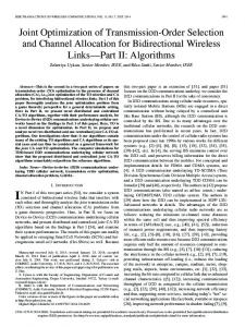
APPENDIX We first introduce some preliminary results instrumental to prove both Theorem 2 and Theorem 3. Given and , for notational simplicity, we will denote by (or interchangeably ) the vector whose component is equal to if , and zero otherwise. With a slight abuse of notation we will also use to ; denote the ordered tuple similarly , with stands for . Fig. 5. Dictionary Learning Problem, 16 cores; objective value vs. time for: , —(b) , . In the subplot (b), some curves (a) are not properly displayed because of overlaps, essentially they all behave like RFLEXA.
RFLEXA, and FLEXA, we compared HyFLEXA also with the algorithm proposed in [45] (cf. Algorithm 2) specifically for the dictionary learning problem. In all the algorithms, the dictionary matrix and sparse representation matrix are initialized with overcomplete DCT dictionary [49] and zero matrix, respectively. Results of our simulations are reported in Fig. 5, where we plot the objective value versus the CPU time. On our tests, different algorithms seem to converge to different points that have been checked to be all stationary. It is interesting that HyFLEXA reaches a lower objective value. It should also be noted that lower objective values correspond to different sparsity-degrees. For example, in the first problem, RFLEXA ( ), SPARSA, and HyFLEXA ] reach a solution with 3223, 3648, [ and 4838 nonzero variables, respectively, which are in the same range of sparsity, but HyFLEXA has a better objective value. Now consider the second problem, where HyFLEXA [ ] and HyFLEXA [ ] reach two different (stationary) point with 1411 and 2064 nonzero variables, respectively, while all the other algorithms converges to the same point with 766 nonzero variables. In conclusion, HyFLEXA seems very competitive, outperforming RFLEXA and comparing very well also to deterministic methods. V. CONCLUSION We proposed a highly parallelizable hybrid random/deterministic decomposition algorithm for the minimization of the sum of a possibly noncovex differentiable function and a possibily nonsmooth nonseparable convex function . The proposed framework is the first scheme enjoying all the following features: i) it allows for pure greedy, pure random, or mixed random/greedy updates of the variables, all converging under the same unified set of convergence conditions; ii) it can tackle via parallel updates also nonseparable convex functions ; iii) it can deal with nonconvex nonseparable ; iv) it is parallel; v) it can incorporate both first-order or higher-order information; and vi) it can use inexact solutions. Our preliminary experiments on LASSO problems and few selected nonconvex ones showed a very promising behavior with respect to state-of-the-art random and deterministic algorithms. Of course, a more complete assessment, especially in the nonconvex case, require much more experiments and is the subject of current research.
A. On the Random Sampling and Its Properties We introduce some properties associated with the random sampling rules satisfying assumption A6. A key role in our proofs is played by the following random set: let be the sequence generated by Algorithm 1, and (12) define the set
as (13)
The key properties of this set are summarized in the following two lemmata. Lemma 5 (Infinite Cardinality): Given the set as in (13), it holds that where denotes the cardinality of . Proof: Suppose that the statement of the lemma is not true. Then, with positive probability, there must exist some such that for , . But we can write
where the inequality follows by A6 and the independence of the events. But this obviously gives a contradiction and concludes the proof. Lemma 6: Let be a sequence satisfying assumptions i)–iii) of Theorem 2. Then it holds that (14) Proof: It holds that,
To prove the lemma, it is then sufficient to show that , as proved next. Define , with , as the smallest index such that (15)
3924
IEEE TRANSACTIONS ON SIGNAL PROCESSING, VOL. 63, NO. 15, AUGUST 1, 2015
Note that since and
, . For any
is well-defined for all , it holds:1
(c) we used the bounds .
and
Term II: Let us rewrite term II as
(16)
Let us bound next “term I” and “term II” separately. Term I: We have
(18)
(17)
where: (a)
B. On the Best-Response Map are independent Bernoulli random vari-
ables, with parameter . Note that, due to A6, , for all ; (b) it follows from Chebyshev’s inequality; 1For
where: (a) we used , by the conditioning event; (b) it follows from (15), and ; (c) are independent Bernoulli random variables, with parameter . The bound is due to ; (d) it follows from the Chebyshev’s inequality. The desired result (14) follows readily combining (16), (17), and (18).
notational simplicity, hereafter we will use
for
.
and Its Properties
We introduce now some key properties of the mapping defined in (6). We also derive some bounds involving along generated by Algorithm 1. with the sequence Lemma 7 ([20]): Consider Problem (1) under A1–A5, and F1–F3. Suppose that is separable, i.e., , with each convex on . Then the mapping
DANESHMAND et al.: HYBRID RANDOM/DETERMINISTIC PARALLEL ALGORITHMS
is Lipschitz continuous on a positive constant such that
, i.e., there exists
3925
along with the gradient consistency condition (cf. F2) imply
(19) be the sequence generated by Algorithm Lemma 8: Let 1. For every and generated as in step S.3 of Algorithm 1, the following holds: there exists a positive constant such that, (20)
(24) To bound the second term on the RHS of (22), let us invoke the : convexity of
Proof: The following chain of inequalities holds:
which yields
where: in (a)
is any index in such that . Note that by definition of (cf. step S.3 of Algorithm 1), such a index always exists; (b) is due to (8); (c) follows from the definition of , and , the latter due to (recall that ); and (d) follows from (8). Lemma 9: Let be the sequence generated by Algorithm 1. For every , and generated as in step S.3, the following holds:
(25) The desired result (21) is readily obtained by combining (22) . with (24) and (25), and summing over Lemma 10: Let be the sequence generated by Algo. For every sufficiently large, and rithm 1, and generated as in step S.3, the following holds:
(26)
Proof: Given
and
, define
, with if otherwise.
(21)
Proof: Optimality of
for all
By the convexity and Lipschitz continuity of
, it follows
for the subproblem implies
(27)
, and some . Therefore,
(22)
is a (global) Lipschitz constant of . We bound next where the last term on the RHS of (27). Let , for large enough so that . , with if , and Define
Let us (lower) bound next the two terms on the RHS of (22). The uniform strong monotonicity of (cf. F1),
(28) otherwise. Using the definition of
(23)
it is not difficult to see that (29)
3926
Using (29) and invoking the convexity of recursion holds for sufficiently large :
IEEE TRANSACTIONS ON SIGNAL PROCESSING, VOL. 63, NO. 15, AUGUST 1, 2015
, the following
and . Then either converges to a finite value and
or else .
C. Proof of Theorem 2 For any given and rithm 1,
, the Descent Lemma [51] yields: with defined in step S.4 of Algo-
(32) We bound next the second and third terms on the RHS of (32). Denoting by
the complement of
, we have,
(30) Using (30), the last term on the RHS of (27) can be upper bounded for sufficiently large as (33)
where in (a) we used the definition of and of the set ; in ; and (c) follows from (29) (cf. (b) we used Lemma 9). The third term on the RHS of (32) can be bounded as (31)
where (a) is due to the convexity of and the definition [cf. (28)]. of The desired inequality (26) follows readily by combining (27) with (31). Lemma 11: [56, Lemma 3.4, p.121] Let , , and be three sequences of numbers such that for all . Suppose that
(34)
where the first inequality follows from the definition of , and in the last inequality we used
and .
DANESHMAND et al.: HYBRID RANDOM/DETERMINISTIC PARALLEL ALGORITHMS
Now, we combine the above results to get the descent property of along . For sufficiently large , it holds
3927
for all and . This implies that, w.p.1, there exists an infinite sequence of indexes, say , such that (40)
(35) where the inequality follows from (21), (32), (33), and (34), and is given by
By assumption (iv) in Theorem 2, it is not difficult to show that . Since , it follows from (35) that there exist some positive constant and a sufficiently large , say , such that
Suppose now, by contradiction, that with a positive probability. Then we can find a realization such that at the same time (40) holds for some and . In the rest of the proof we focus on this realization and get a contradiction, thus proving that w.p.1. If then there exists a such that for infinitely many and also for infinitely many . Therefore, one can always find an infinite set of indexes, say , having the following , there exists an integer such properties: for any that (41)
(36) . Invoking Lemma 11 while using for all and the coercivity of , we deduce from (36) that
(42) Proceeding now as in the proof of Theorem 2 in [20], we have: , for
(37) (43) and thus also
(44) (38)
Lemma 6 together with (38) imply
(45)
which by Lemma 8 implies (39) Therefore, the limit point of the infimum sequence is a fixed w.p.1. point of
where (a) follows from (41); (b) is due to Lemma 7; (c) comes from the triangle inequality, the updating rule of the algorithm and the definition of ; and in (d) we used (41), (42), and , where . It follows from (45) that (46)
D. Proof of Theorem 3 The proof follows similar ideas as the one of Theorem 1 in our recent work [20], but with the nontrivial complication of dealing with randomness in the block selection. Given (39), we show next that, under the separability assumption on , it holds that w.p.1. For . notational simplicity, let us define Note first that for any finite but arbitrary sequence , it holds that
We show next that (46) is in contradiction with the convergence of . To do that, we preliminary prove that, for sufficiently large , it must be . Pro, ceeding as in (45), we have: for any given
It turns out that for sufficiently large , it must be
so that (47)
and thus
otherwise the condition would be violated [cf. (42)]. Hereafter we assume without loss of generality that (47) holds for all (in fact, one can always restrict to a proper subsequence).
3928
IEEE TRANSACTIONS ON SIGNAL PROCESSING, VOL. 63, NO. 15, AUGUST 1, 2015
We can show now that (46) is in contradiction with the convergence of . Using (36) (possibly over a subse, quence), we have: for sufficiently large
(48) where (a) follows from Lemma 8 and ; and (b) . is due to (47) and (48), with Since converges and , it holds , contradicting (46). Therefore that w.p.1. Since is bounded by and the convergence of , it has the coercivity of at least one limit point . By the continuity of (cf. Lemma 7) it holds that . By Proposition 1 is also a stationary solution of Problem (1). ACKNOWLEDGMENT The authors are very grateful to Prof. Peter Richtàrik for his invaluable comments; we also thank Dr. Martin Takáč and Prof. Peter Richtàrik for providing the C++ code of PCDM and (that we modified in order to use the MPI library). REFERENCES [1] A. Daneshmand, F. Facchinei, V. Kungurtsev, and G. Scutari, “Flexible selective parallel algorithms for big data optimization,” in Proc. 48th Asilomar Confe. Signals, Syst., Comput., Nov. 2–5, 2014, pp. 3–7. [2] R. Tibshirani, “Regression shrinkage and selection via the lasso,” J. Roy. Statist. Soc. B (Methodol.), pp. 267–288, 1996. [3] Z. Qin, K. Scheinberg, and D. Goldfarb, “Efficient block-coordinate descent algorithms for the group lasso,” Math. Programm. Comput., vol. 5, pp. 143–169, June 2013. [4] G.-X. Yuan, K.-W. Chang, C.-J. Hsieh, and C.-J. Lin, “A comparison of optimization methods and software for large-scale l1-regularized linear classification,” J. Mach. Learn. Res., vol. 11, pp. 3183–3234, 2010. [5] K. Fountoulakis and J. Gondzio, “A second-order method for strongly convex L1-regularization problems,” 2013, arXiv preprint arXiv:1306. 5386 [Online]. Available: http://arxiv.org/abs/1306.5386 [6] I. Necoara and D. Clipici, “Efficient parallel coordinate descent algorithm for convex optimization problems with separable constraints: Application to distributed MPC,” J. Process Control, vol. 23, no. 3, pp. 243–253, March 2013. [7] Y. Nesterov, “Gradient methods for minimizing composite functions,” Math. Programm., vol. 140, pp. 125–161, August 2013. [8] P. Tseng and S. Yun, “A coordinate gradient descent method for nonsmooth separable minimization,” Math. Programm., vol. 117, no. 1–2, pp. 387–423, March 2009. [9] A. Beck and M. Teboulle, “A fast iterative shrinkage-thresholding algorithm for linear inverse problems,” SIAM J. Imag. Sci., vol. 2, no. 1, pp. 183–202, Jan. 2009. [10] S. J. Wright, R. D. Nowak, and M. A. Figueiredo, “Sparse reconstruction by separable approximation,” IEEE Trans. Signal Process., vol. 57, no. 7, pp. 2479–2493, Jul. 2009. [11] Z. Peng, M. Yan, and W. Yin, “Parallel and distributed sparse optimization,” in Proc. Asilomar Conf. IEEE Signals, Syst., Comput., 2013, pp. 659–646. [12] K. Slavakis and G. B. Giannakis, “Online dictionary learning from big data using accelerated stochastic approximation algorithms,” presented at the IEEE Int. Conf. Acoust., Speech, Signal Process. (ICASSP), Florence, Italy, May 4–9, 2014.
[13] K. Slavakis, G. B. Giannakis, and G. Mateos, “Modeling and optimization for big data analytics,” IEEE Signal Process. Mag., vol. 31, no. 5, pp. 18–31, Sep. 2014. [14] M. De Santis, S. Lucidi, and F. Rinaldi, ‘A fast active set block coordinate descent algorithm for -regularized least squares,” Mar. 2014, eprint arXiv:1403.1738 [Online]. Available: http://arxiv.org/abs/1403. 1738 [15] , S. Sra, S. Nowozin, and S. J. Wright, Eds., Optimization for Machine Learning, ser. Neural Information Processing. Cambridge, MA, USA: MIT Press, Sep. 2011. [16] F. Bach, R. Jenatton, J. Mairal, and G. Obozinski, “Optimization with sparsity-inducing penalties,” Found. Trends Mach. Learn., vol. 4, no. 1, pp. 1–106, 2011. [17] J. K. Bradley, A. Kyrola, D. Bickson, and C. Guestrin, “Parallel coordinate descent for l1-regularized loss minimization,” presented at the 28th Int. Conf. Mach. Learn., Bellevue, WA, USA, Jun. 28–Jul. 2, 2011. [18] M. Patriksson, “Cost approximation: A unified framework of descent algorithms for nonlinear programs,” SIAM J. Optim., vol. 8, no. 2, pp. 561–582, 1998. [19] F. Facchinei, S. Sagratella, and G. Scutari, “Flexible parallel algorithms for big data optimization,” presented at the IEEE Int. Conf. Acoust., Speech, Signal Process. (ICASSP), Florence, Italy, May 4–9, 2014. [20] F. Facchinei, S. Sagratella, and G. Scutari, “Flexible parallel algorithms for big data optimization,” IEEE Trans. Signal Process. vol. 63, no. 7, pp. 1874–1889, Apr. 2015. [21] O. Fercoq, Z. Qu, P. Richtárik, and M. Takáč, “Fast distributed coordinate descent for non-strongly convex losses,” 2014, arXiv preprint arXiv:1405.5300 [Online]. Available: http://arxiv.org/abs/1405.5300 [22] O. Fercoq and P. Richtárik, “Accelerated, parallel and proximal coordinate Descent,” 2013, arXiv preprint arXiv:1312.5799 [Online]. Available: http://arxiv.org/abs/1312.5799 [23] Z. Lu and L. Xiao, “Randomized block coordinate non-monotone gradient method for a class of nonlinear programming,” 2013, arXiv preprint arXiv:1306.5918v1 [Online]. Available: http://arxiv.org/pdf/1306.5918.pdf [24] I. Necoara and D. Clipici, “Distributed random coordinate descent method for composite minimization,” Tech. Rep., Nov. 2013, pp. 1–41 [Online]. Available: http://arxiv-web.arxiv.org/abs/1312.5302 [25] Y. Nesterov, “Efficiency of coordinate descent methods on huge-scale optimization problems,” SIAM J. Optim., vol. 22, no. 2, pp. 341–362, 2012. [26] P. Richtárik and M. Takáč, “Parallel coordinate descent methods for big data optimization,” 2012, arXiv preprint arXiv:1212.0873 [Online]. Available: http://arxiv.org/abs/1212.0873 [27] S. Shalev-Shwartz and A. Tewari, “Stochastic methods for -regularized loss minimization,” J. Mach. Learn. Res., pp. 1865–1892, 2011. [28] Z. Lu and L. Xiao, “On the complexity analysis of randomized blockcoordinate descent methods,” 2013, arXiv preprint arXiv:1305.4723 [Online]. Available: http://arxiv.org/abs/1305.4723 [29] I. Necoara and A. Patrascu, “A random coordinate descent algorithm for optimization problems with composite objective function and linear coupled constraints,” Comput. Optim. Appl., vol. 57, no. 2, pp. 307–337, 2014. [30] A. Patrascu and I. Necoara, “Efficient random coordinate descent algorithms for large-scale structured nonconvex optimization,” J. Global Optim., pp. 1–23, Feb. 2014. [31] P. Richtárik and M. Takáč, “Iteration complexity of randomized block-coordinate descent methods for minimizing a composite function,” Math. Programm., vol. 144, no. 1–2, pp. 1–38, 2014. [32] I. Dassios, K. Fountoulakis, and J. Gondzio, “A second-order method for compressed sensing problems with coherent and redundant dictionaries,” 2014, arXiv preprint arXiv:1405.4146 [Online]. Available: http://arxiv.org/abs/1405.4146 [33] G.-X. Yuan, C.-H. Ho, and C.-J. Lin, “An improved glmnet for -regularized logistic regression,” J. Mach. Learn. Res., vol. 13, no. 1, pp. 1999–2030, 2012. [34] G. Scutari, F. Facchinei, P. Song, D. Palomar, and J.-S. Pang, “Decomposition by Partial linearization: Parallel optimization of multi-agent systems,” IEEE Trans. Signal Process., vol. 62, pp. 641–656, Feb. 2014. [35] C. Scherrer, A. Tewari, M. Halappanavar, and D. Haglin, Curran Associates, Inc., “Feature clustering for accelerating parallel coordinate descent,” in Adv. Neural Inf. Process. Syst. (NIPS), 2012, pp. 28–36. [36] A. Auslender, Optimisation: Méthodes Numériques. Paris, France: Masson, 1976. [37] P. Tseng, “Convergence of a block coordinate descent method for nondifferentiable minimization,” J. Optim. Theory Appl., vol. 109, no. 3, pp. 475–494, 2001. [38] M. Razaviyayn, M. Hong, and Z.-Q. Luo, “A unified convergence analysis of block successive minimization methods for nonsmooth optimization,” SIAM J. Opt., vol. 23, no. 2, pp. 1126–1153, 2013.
DANESHMAND et al.: HYBRID RANDOM/DETERMINISTIC PARALLEL ALGORITHMS
[39] M. Razaviyayn, M. Hong, Z.-Q. Luo, and J.-S. Pang, “Parallel successive convex approximation for nonsmooth nonconvex optimization,” presented at the Annu. Conf. Neural Inf. Process. Syst. (NIPS), Montreal, QC, Canada, Dec. 2014, to appear. [40] M. Hong, M. Razaviyayn, and Z.-Q. Luo, “Convergence analysis of alternating direction method of multipliers for a family of nonconvex problems,” Oct. 2014, arXiv preprint arXiv:1410.1390 [Online]. Available: http://arxiv.org/abs/1410.1390 [41] J. T. Goodman, “Exponential priors for maximum entropy models,” U.S. Patent 7 340 376, Mar. 4, 2008. [42] K.-W. Chang, C.-J. Hsieh, and C.-J. Lin, “Coordinate descent method for large-scale l2-loss linear support vector machines,” J. Mach. Learn. Res., vol. 9, pp. 1369–1398, 2008. [43] R. Tappenden, P. Richtárik, and J. Gondzio, “Inexact coordinate descent: Complexity and preconditioning,” 2013, arXiv preprint arXiv:1304.5530 [Online]. Available: http://arxiv.org/abs/1304.5530 [44] P. Richtárik and M. Takáč, “Distributed coordinate descent method for learning with big data,” 2013, arXiv preprint arXiv:1310.2059 [Online]. Available: http://arxiv.org/abs/1310.2059 [45] M. Razaviyayn, H.-W. Tseng, and Z.-Q. Luo, “Dictionary learning for sparse representation: Complexity and algorithms,” presented at the IEEE Int. Conf. Acoust., Speech, Signal Process. (ICASSP), Florence, Italy, May 4–9, 2014. [46] T. Hastie, R. Tibshirani, and J. Friedman, The Elements of Statistical Learning, ser. Springer Series in Statistics. New York, NY, USA: Springer, 2009. [47] H. A. Eiselt and V. Marianov, “Pioneering developments in location analysis,” in Foundations of Location Analysis, International Series in Operations Research & Management Science, A. Eiselt and V. Marianov, Eds. New York, NY, USA: Springer, 2011, ch. 11, pp. 3–22. [48] A. Chambolle, “An algorithm for total variation minimization and applications,” J. Math. Imag. Vis., vol. 20, no. 1–2, pp. 89–97, Jan. 2004. [49] J. Mairal, F. Bach, J. Ponce, and G. Sapiro, “Online Dictionary Learning for Sparse Coding,” in Proc. 26th Int. Conf. Mach. Learn., Montreal, QC, Canada, Jun. 14–18, 2009. [50] D. Goldfarb, S. Ma, and K. Scheinberg, “Fast alternating linearization methods for minimizing the sum of two convex functions,” Math. Programm., vol. 141, pp. 349–382, Oct. 2013. [51] D. P. Bertsekas and J. N. Tsitsiklis, Parallel and Distributed Computation: Numerical Methods, 2nd ed. Belmont, MA, USA: Athena Scientific, 1989. [52] J.-S. Pang, “Error bounds in mathematical programming,” Math. Programm., vol. 79, no. 1–3, pp. 299–332, 1997. [53] P. Richtárik and M. Takáč, “On optimal probabilities in stochastic coordinate descent methods,” 2013, arXiv preprint arXiv:1310.3438 [Online]. Available: http://arxiv.org/abs/1310.3438 [54] A. Daneshmand, “Numerical comparison of hybrid random/deterministic parallel algorithms for nonconvex big data optimization,” Dept. of Elect. Eng., SUNY Buffalo, Buffalo, NY, USA, Tech. Rep., Aug. 2014 [Online]. Available: http://www.eng.buffalo.edu/∼amirdane/DaneshmandTechRepNumCompAug14.pdf [55] CBCL Face Database #1, MIT Center for Biological and Computation Learning [Online]. Available: http://www.ai.mit.edu/projects/cbcl [56] D. P. Bertsekas and J. N. Tsitsiklis, Neuro-Dynamic Programming. Cambridge, MA, USA: Athena Scientific, May 2011. Amir Daneshmand received his B.Sc. and M.Sc. degree in electrical engineering from Tehran Polytechnic (2013) and State University of New York at Buffalo (2015). He is currently a Ph.D. in the Department of Electrical Engineering at the State University of New York at Buffalo, NY. His research interests include big data optimization, distributed/decentralized optimization over networks, and higher order tensor analysis and its applications."
3929
Francisco Facchinei received the Ph.D. degree in system engineering from the University of Rome, “La Sapienza,” Rome, Italy. He is full professor of Operations Research, Engineering Faculty, University of Rome, “La Sapienza.” His research interests focus on theoretical and algorithmic issues related to nonlinear optimization, variational inequalities, complementarity problems, equilibrium programming, and computational game theory.
Vyacheslav Kungurtsev was born in St. Petersburg, Russia, in 1986, and immigrated to the United States in 1993. He received his B.S. in Mathematics from Duke University in 2007 and his Ph.D. from UC-San Diego in Mathematics with a specialization in Computational Science in 2013. Subsequently he spent one year as a postdoctoral fellow at the Optimization for Engineering Center (OPTEC) at KU Leuven in Belgium, and is currently a postdoctoral fellow at the Agents Technology Center in the Faculty of Computer Science in the department of Electrical Engineering at Czech Technical University in Prague. His research interests include a broad scope of problems in continuous optimization and its applications.
Gesualdo Scutari (S’05–M’06–SM’11) received the Electrical Engineering and Ph.D. degrees (both with honors) from the University of Rome “La Sapienza”, Rome, Italy, in 2001 and 2005, respectively. He is an Associate Professor with the School of Industrial Engineering at Purdue University. He had previously held several research appointments, namely, at University of California at Berkeley, Berkeley, CA; Hong Kong University of Science and Technology, Hong Kong; University of Rome, “La Sapienza”, Rome, Italy; University of Illinois at Urbana-Champaign, Urbana, IL. His primary research interests focus on theoretical and algorithmic issues related to large-scale optimization, equilibrium programming, and their applications to signal processing, medical imaging, machine learning, networking, and distributed decisions. Dr. Scutari is an Associate Editor of IEEE TRANSACTIONS ON SIGNAL PROCESSING and he served as an Associate Editor of IEEE SIGNAL PROCESSING LETTERS. He serves on the IEEE Signal Processing Society Technical Committee on Signal Processing for Communications (SPCOM). Dr. Scutari received the 2006 Best Student Paper Award at the International Conference on Acoustics, Speech and Signal Processing (ICASSP) 2006, the 2013 NSF Faculty Early Career Development (CAREER) Award, and the 2013 UB Young Investigator Award.