Compressible large-eddy simulations of turbulent flow over a wall-mounted hump with active ... The flow is characterized by the unsteady separation before the.
AIAA JOURNAL Vol. 48, No. 6, June 2010
Compressible Large-Eddy Simulation of Separation Control on a Wall-Mounted Hump Jennifer A. Franck∗ and Tim Colonius† California Institute of Technology, Pasadena, California 91125 DOI: 10.2514/1.44756 Compressible large-eddy simulations of turbulent flow over a wall-mounted hump with active flow control are performed and compared with previous experiments. The flow is characterized by the unsteady separation before the steep trailing edge, which naturally reattaches downstream of the hump to form an unsteady turbulent separation bubble. The low Mach number large-eddy simulation demonstrated a good prediction of surface pressure coefficient, separation-bubble length, and velocity profiles compared with experiments. The effect of compressibility on the baseline flow is documented and analyzed and is found to increase the separation-bubble size, due to a reduced growth rate. Control is applied just before the natural separation point via steady suction and zero-net-mass-flux oscillatory forcing, and steady suction is shown to be more effective in decreasing the size of the separation bubble and pressure drag for the control parameters investigated. Controlled flow at a compressible subsonic Mach number is applied, and found to be slightly less effective than the same control parameters at low Mach numbers.
performed an implicit LES (ILES) on the baseline and controlled cases at a Reynolds number of 200,000: one-fifth of the Reynolds number of the Langley Research Center Workshop (LRCW) test case. Good agreement was found between the pressure coefficient in the baseline and steady-suction control cases; however, the separation-bubble length was overpredicted in the oscillatory forcing. Increasing the magnitude of oscillatory forcing improved the separation-bubble length, agreeing with the trend in experimental data. Saric et al. [7] found better agreement with the experiments using LES rather than RANS or detached eddy simulation, which overpredicted the reattachment location. The dynamic Smagorinsky model of You et al. [8] best predicted the wall-pressure coefficient and separation-bubble length for the oscillatory-control case. All the previous simulations, including those solving the compressible equations, have focused on the low Mach number (M � 0:1) results from the LRCW test case. Seifert and Pack [2] have investigated the flow over a range of Mach numbers from 0.25 to 0.7 and observed the effect of compressibility on the baseline and controlled flow. The numerical method presented in this paper is a compressible LES capable of modeling the compressible subsonic flow over the hump with improved numerical robustness from a previous ILES [9]. Baseline flow is explored for incompressible and compressible Mach numbers of 0.25 and 0.6, respectively, and compared with available data from both the LRCW experiments and those performed by Seifert and Pack [2]. Steady suction and oscillatory forcing are applied to simulate the controlled experiments and validate our numerical control method. The dynamics and the effects of compressibility on the baseline and controlled flow are also discussed.
I. Introduction
S
YNTHETIC jets have been shown to increase aerodynamic performance of naturally separating flows in laboratory experiments. However, the development of accurate predictive tools for unsteady separation and control remains a challenge, especially at high Reynolds numbers [1]. To provide an experimental database of separated and controlled flows that can be used for computational validation, Seifert and Pack [1,2] investigated the turbulent flow over a wall-mounted hump geometry. At fully turbulent Reynolds numbers the wall-mounted hump flow is characterized by its unsteady separation bubble that forms over the trailing edge. Seifert and Pack investigated many control configurations, including steady-suction and oscillatory zero-net-mass-flux control, over a range of Mach numbers. The wall-mounted hump was also a test case at the CFD Validation of Synthetic Jets and Turbulent Separation Control workshop held at NASA Langley Research Center (LaRC) [3]. The workshop provided a separate set of experimental data of the baseline and controlled flow including additional data from pressure taps, particle image velocimetry (PIV), and oil-film flow visualization along the surface of the hump [4,5]. The welldocumented experiments from both groups provide a database that can be used for the development of computational fluid dynamics (CFD) techniques capable of simulating separation and control. Participants from the workshop simulated the wall-mounted hump flow using a variety of techniques, including Reynolds-averaged Navier–Stokes (RANS) and large-eddy simulation (LES) [3]. These methods displayed varying degrees of success in predicting the surface pressure coefficient of the baseline, steady-suction, and oscillatory-control test cases at a Reynolds number of 9:29 � 105 based on the freestream velocity U1 and the chord length c. It has been shown that LES generally provides better agreement with the experimental reattachment location and separation-bubble dynamics than RANS-based simulations [6,7]. In particular, Morgan et al. [6]
II. Computational Methodology The governing equations are the density-weighted, low-passfiltered, three-dimensional, compressible Navier–Stokes equations:
Presented as Paper 555 at the 46th AIAA Aerospace Sciences Meeting and Exhibit, Reno, NV, 7–10 January 2008; received 5 April 2009; revision received 22 February 2010; accepted for publication 26 February 2010. Copyright © 2010 by Jennifer A. Franck and Tim Colonius. Published by the American Institute of Aeronautics and Astronautics, Inc., with permission. Copies of this paper may be made for personal or internal use, on condition that the copier pay the $10.00 per-copy fee to the Copyright Clearance Center, Inc., 222 Rosewood Drive, Danvers, MA 01923; include the code 0001-1452/ 10 and $10.00 in correspondence with the CCC. ∗ Division of Engineering and Applied Sciences; currently Brown University, Division of Engineering. Member AIAA. † Professor, Division of Engineering and Applied Sciences, Mechanical Engineering. Senior Member AIAA.
@ @�� � �� u~ � 0 @xj j @t
(1a)
@ @p� @ sgs @ �� u~ i � ��� u~ i u~ j � �~ji � � � � @xj @xi @xj ij @t
(1b)
@ @ sgs @ ~ � u~ j � q~ j � �~ji u~ i � � �� E � ���� E~ �p� q @xj @xj j @t
(1c)
where f� is a low-pass-filtered variable, and the density-weighted filtered variable f~ is defined by 1098
1099
FRANCK AND COLONIUS
1
The length scales are nondimensionalized by the chord length c, the velocities are nondimensionalized by the speed of sound a1 , and the pressure is nondimensionalized by �a21. The dynamic viscosity is held constant, the Prandtl number is fixed at 0.7, and the ideal-gas law is used as the equation of state. The filtered stress tensor and heat flux vector components are defined by �~ ij � 2��S~ij � 1=3S~kk �ij �
� @T~ Pr @xj
�
~ S~ij � Sj 2Cs2 �2 �j
0 1
2
3
@���E � p�uj � 1 @��euj � �uj @e e @��uj � ! � � 2 @xj @xj 2 @xj 2 @xj �
(5)
(6)
(7)
~ � �2S~ij S~ij �1=2 . and jSj The governing equations are solved in a computational domain with the generalized coordinates � � f�x; y� and � � f�x; y� in the streamwise and wall-normal directions. A conformal mapping from the computational domain (� � � � i�) to the physical domain (z � x � iy) is calculated using the Schwartz–Christoffel Toolbox by Driscoll and Trefethen [11], capable of creating a conformal mapping from the equally spaced rectangular computational grid to an arbitrary physical grid defined by polygon vertices. The current hump geometry is defined by approximately 900 vertices denoted by the contour � � 0. The smooth contour line just above the polygon boundary at � � � is used as the lower boundary of the physical grid. Many numerical methods for LES employ explicit filtering on the smallest resolved scales in the flow. Some use explicit filtering in lieu of traditional SGS models (e.g., implicit LES, ILES) or because low dissipation, high-order finite difference schemes are used. For the latter, energy buildup at scales near the grid cutoff can lead to numerical instabilities in the absence of filtering. In an earlier version of our algorithm, we employed such filtering in combination with the above Smagorinsky model as well as a dynamic Smagorinsky model [12]. Our experience was that the aggressive filtering that was required to render the solution stable, even on a relatively fine mesh, was overly dissipative and rendered the turbulence model superfluous. In an attempt to alleviate the need for explicit filtering, the current LES controls energy buildup through a conservative method implemented with a skew-symmetric formulation [13] of the convective terms given by Eqs. (8) and (9), where e is the internal energy and E � e � 1=2�uj uj �: @��ui uj � 1 @��ui uj � �uj @ui ui @��uj � ! � � @xj 2 @xj 2 @xj 2 @xj
N = 3, α f = 0.40 N = 4, α f = 0.35 N = 4, α f = 0.49
0.2
(4)
where Cs and Cq are constant model coefficients. A value of approximately 0.17 is used for both model coefficients [10]. The filtered rate of strain S~ij is � � 1 @u~ i @u~ j � S~ ij � 2 @xj @xi
0.4
k Fig. 1 Transfer function of commonly used explicit filters from Eq. (10).
and ~ 2 ~ @T � Sj qsgs j � Cq � �j @xj
0.6
0
The subgrid-scale (SGS) terms �ijsgs and qsgs j are modeled using the Smagorinsky formulation given by �ijsgs
0.8
(3)
and q~ j � �
1.2
(2)
T (k)
�f f~ � ��
(8)
1 @��ui ui uj � @�puj � � 2 @xj @xj
(9)
Time-stepping is accomplished with a fourth-order Runge–Kutta scheme. A Fourier spectral method is implemented in the z direction, since the geometry of interest is homogeneous across the span. A sixth-order-accurate explicit finite difference scheme is implemented in the streamwise and wall-normal directions. The third-orderaccurate boundary closures are derived from summation by parts (SBP) operators based on diagonal norms [14]. Because of the proven stability properties of the SBP operators and the skewsymmetric convective terms the current solver is more robust than our previous sixth-order compact finite difference method [9]. The convergence of the numerical method, in the absence of the SGS model, was confirmed with simple acoustic pulse and vortex advection flows. With the SBP finite difference scheme and skew-symmetric formulation, we find that we are able to run stable solutions on underresolved meshes without filtering. For grids such as the current one with aggressive grid clustering in the boundary layer, we still find an undesirable contamination of the solution with grid-point to gridpoint oscillations (even though it results in long-term stability). We find that these oscillations are easily controlled with explicit filtering, but, by comparison to the previous formulation, with a much less aggressive filter. Thus, in production calculations, the high-order spatial filter [15] given by Eq. (10) was applied in the wall-normal and spanwise directions after every full time step. The filter parameter f was set to 0.49, which provides a suitably sharp Fourier cutoff. This filter is shown in Fig. 1, alongside more aggressive filters that were used to damp numerical instabilities in the aforementioned earlier version of the algorithm: 4 1X a �f � fi�n � f �f^i�1 � f^i�1 � � 2 n�0 N i�n
III.
(10)
Simulation Details
The geometry investigated is a wall-mounted hump that approximates the upper surface of a 20%-thick Glauert– Goldschmied-type airfoil. The domain size shown in Fig. 2 is 4:9c � 0:909c � 0:2c and is shorter than the experimental domain in the spanwise and streamwise directions in order to reduce the computational cost. The grid is shown in Fig. 3 with every sixth grid point plotted. The grid points are highly clustered around the separation region and along the wall using a hyperbolic stretching function [16], with ��x=c�min � 4:04 � 10�4 and ��y=c�min � 4:39 � 10�4 . Current computations have 800 grid points in the
1100
FRANCK AND COLONIUS
Fig. 2
number is lower than the LRCW test cases, but it is within the range of Reynolds numbers investigated experimentally [4]. Rather than model the flowfield inside the actuation cavity of the experiment, the boundary conditions are modified at the wall to simulate the slot jet [8,22]. When actuation is applied a normal velocity distribution is prescribed on the boundary nodes to approximate the same slot location and approximate slot width as used in the experiments. The slot geometry and location from Greenblatt et al. [4] is shown in Fig. 4 with the slot region enlarged. Superimposed over the slot are the grid points that define the forcing width and location depicted as the positive normal velocity imposed during the blowing phase. The velocity at the wall, us , is given by the Gaussian profile:
LES computational domain.
0.5
us �x� � us;max e��x�xs � -1
0
1
2
3
x/c Fig. 3 LES computational grid with every sixth grid point plotted.
streamwise direction, 160 in the wall-normal direction, and 64 points in the spanwise direction, for a total of approximately 8.2 million points. As with any LES model, grid convergence can only be achieved in terms of a statistical correspondence with the filtered DNS field [17]. However, given the intractable computational costs of such a simulation, a full grid resolution study is not performed. Instead, the resolution of the LES is assessed by creating a coarser mesh with half as many grid points in each coordinate direction, the results of which are presented in Sec. IV.A. The primary goal of this work is to investigate the flow separation and reattachment downstream of the hump, therefore we do not attempt to fully resolve the inflow turbulent boundary layer. The resolution at the point x=c � �0:5 on the wall is �x=c � 9:4 � 10�3 , �y=c � 8:7 � 10�4 , and �z=c � 3:1 � 10�3 in the streamwise, wall-normal, and spanwise directions, respectively, corresponding to �x� � 94, �y� � 8:7, and �z� � 31. Although the spatial resolution of the boundary layer is coarse for a turbulent boundarylayer simulation, the grid spacing decreases significantly close to separation, the region of interest for this investigation. It is noted that computations of the skin-friction coefficient are underpredicted, due to the underresolution of the viscous sublayer, but the trends agree qualitatively with the experiments [18]. Overall, due to the good prediction of the flow physics surrounding separation and reattachment, the resolution is found to be sufficient for the current investigation. The time step is �ta1 =c � 3:5 � 10�4 for the M � 0:6 cases and �ta1 =c � 4:5 � 10�4 for the M � 0:25 cases. Baseline simulations are run until the flow is fully developed, and time-averaged results are calculated over the subsequent 5–10 c=U1 . Controlled cases are started from a fully developed baseline flow. The flow is initialized with a potential flow solution superimposed with a turbulent boundary-layer profile on the lower wall, which closely matches the experimental profile obtained by Greenblatt et al. [4]. Although the profile is matched, the upstream boundary-layer thickness is smaller than in the experiments. However, it has been shown by Seifert and Pack [1] that the upstream boundary-layer thickness at high Reynolds numbers has a minor effect on the separation and reattachment dynamics downstream of the hump geometry. To sustain turbulence, velocity perturbations are prescribed at every time step within a Gaussian region close to the inlet, as shown in Fig. 2. The perturbations are formulated by sums of random Fourier modes, an approach used in previous studies [19,20] to accelerate the development of a turbulent boundary layer. The boundary conditions are periodic in the spanwise direction, no-slip, and isothermal conditions on the lower wall boundary, and symmetry is imposed on the upper boundary. The inflow and exit boundaries have nonreflecting boundary conditions with a buffer zone that relaxes the flow toward the initial solution [21]. The Reynolds number of the simulations is 500,000, based on the chord and freestream velocity, unless otherwise noted. The Reynolds
2 =2�h =4�2 s
(11)
where the slot width hs is 0.0055 and the maximum slot velocity at the center of the Gaussian is us;max . The slot width is slightly larger than measured in the LRCW experiments to obtain a well-resolved velocity profile during actuation. When steady-suction actuation is applied the negated velocity profile in Eq. (11) is gradually turned on with the ramp function: r�t� � 12�1 � tanh�3t � 12��
(12)
For oscillatory forcing, the maximum slot velocity is actuated in time by us;max �t� � Us sin�2 ft�
(13)
such that the mean slot velocity is zero for a frequency of f � 1:68U1 =c. The amplitude of the slot velocity oscillation Us controls the amount of momentum added to the flow. The steady-suction-controlled cases can be characterized by the mass-flux coefficient Cm and the steady momentum flux coefficient C� defined in Eq. (14). These values are calculated using the average, or bulk, slot velocity us;b. The magnitude of the velocity profile is set to achieve a Cm value of 0.15% for steady-suction actuation. The nondimensional parameters for the oscillatory control are defined in Eq. (15). The unsteady momentum flux coefficient hC� i is set to 0.11%, and the reduced frequency is F� � 0:84. The reference separation bubble is held constant at xsep � c=2, which is consistent with the F� values of Seifert and Pack [1]. It is noted that Greenblatt et al. [4] report different reduced frequencies, due to a larger value of xsep . Therefore, all reduced frequencies in this manuscript are normalized using xsep � c=2 to allow for a better comparison:
0.2
y/c
0
0.1 0 0
1
0.5
x/c a) Experimental hump and control slot geometry
0.12
y/c
y/c
1
0.11
0.1 0.62
0.64
0.66
0.68
x/c b) Prescribed velocity profile Fig. 4 Experimental hump configuration with an enlargement of the slot geometry and the prescribed Gaussian profile superimposed.
1101
FRANCK AND COLONIUS
Cm �
�s us;b hs ; �1 U1 c
hCm i �
C� �
�s hus;max i2 hs ; 2 0:5�1 U1 c
�s u2s;b hs 2 0:5�1 U1 c
(14)
fxsep U1
(15)
F� �
-1 -0.8 -0.6
Cp
IV. Baseline Flow A.
-0.4
Validation of Baseline Flow
The wall-mounted hump flow has been investigated by two experimental groups using separate wind-tunnel facilities [1,4]. Figure 5 shows the surface pressure coefficient Cp , demonstrating similar results for low Mach number flow at both facilities. The LRCW test case has a higher suction peak at midchord, which may be attributed to the lower wind-tunnel height, creating more blockage. Another facility difference is accounted for by the endplates installed on the LRCW model. When the endplates were temporarily removed the new Cp curve was consistently a better match to the CFD results presented at the workshop [4]. Since the controlled cases are performed with endplates, corresponding experimental Cp results from Greenblatt et al. [4,5] are rescaled by increasing the reference pressure by 0.0365%. This value is obtained by adjusting p1 of the baseline case with endplates until the Cp curve was aligned with the no-endplate baseline case. The result of adjusting p1 for the baseline case is shown in Fig. 5. The experimental data have shown that the baseline flow’s separation and reattachment locations are relatively insensitive to Mach numbers in the range 0.1–0.25, Reynolds number above 517,000 (not shown) [4], and the wind-tunnel model and facility. The boundary layer accelerates over the leading edge of the hump with a small separation bubble at x=c � 0 and reaches a suction peak at x=c � 0:5, initiating pressure recovery. Recovery is hindered when the flow separates at x=c � 0:66, forming an unsteady separation bubble over the trailing edge. As the separated shear layer grows it is deflected toward the wall and eventually reattaches downstream of the hump geometry. For comparison, a fully attached flow over the hump geometry [1] has strong suction peak of Cp � �1:6 at x=c � 0:65 followed by a complete sharp recovery to Cp � 0:5. The LES pressure coefficient of the baseline flow is given in Fig. 6 for a low M � 0:25 and high 0.6 M number and compared with experimental results. At low Mach number, the LES maintains a good prediction of the separation behavior except for a slight overprediction of the pressure coefficient within the separated region. The suction peak at midchord is also lower than the
-0.2 0
M = 0.1 LRCW M = 0.25 S&P M = 0.25 LES M = 0.6 S&P M = 0.6 LES
0.2
0
0.5
1
1.5
x/c Fig. 6 Baseline LES (Re � 0:5 � 106 ) compared with experimental data from Seifert and Pack [1] (S&P) (M � 0:25, Re � 16 � 106 , and M � 0:6, Re � 30 � 106 ) and LRCW [4] (M � 0:1, Re � 1 � 106 ) data without endplates.
experiments, but is not believed to significantly effect the separation dynamics. The LES results show a smaller suction peak within the separated region at the same location as the experimental data, and the slope of the pressure recovery is slightly underpredicted. As the Mach number is increased, the flow has a greater acceleration over the leading edge resulting in a stronger suction peak at midchord. The flow separates at the same physical location but has a lower pressure coefficient at separation and throughout the separated region. The higher Mach number flow has a delayed reattachment and larger separation bubble. The LES captures the main effects of compressibility but overpredicts the pressurerecovery location with less accuracy than the lower Mach number case. This may be partially due to sparser grid resolution at the high Mach reattachment location, since the same grid is used for both cases and was optimized for the low Mach number flow. A lower resolution case with 400 � 80 � 32 grid points is performed for the low Mach number baseline flow, and the average pressure coefficient is compared with the high-resolution case in Fig. 7. With increased resolution, there is improvement in the prediction of the pressure coefficient at separation and improved
M M M M
-1 -1 -0.8
= 0.1 LRCW = 0.25 S&P = 0.25 high res = 0.25 low res
-0.8 -0.6 -0.6
Cp
Cp
-0.4 -0.4
-0.2 -0.2 0 0
M = 0.1 LRCW with endplates M = 0.1 LRCW no endplates M = 0.25 S&P M = 0.1 LRCW adjusted p∞
0.2
0
0.5
1
0.2 1.5
x/c Fig. 5 Surface Cp illustrating facility dependence between Seifert and Pack [1] (S&P) (M � 0:25, Re � 16 � 106 ) and the LRCW [4] (M � 0:1, Re � 1 � 106 ) data. The effect of rescaling p1 for the baseline flow with endplates is compared with the baseline flow without endplates.
0
0.5
1
1.5
x/c Fig. 7 Baseline LES for two different spanwise resolutions of the LES at low Mach number: 800 � 160 � 64 (high resolution), 400 � 80 � 32 (low resolution).
1102
FRANCK AND COLONIUS
x/c = 0.8
The average streamlines in Fig. 10 show the increased separationbubble length for the M � 0:6 flow compared with the low Mach number flow. The delay is reattachment is consistent with the delayed pressure recovery in Fig. 6. Comparing the average streamline corresponding to reattachment, the higher Mach number flow has a separation-bubble length 9.3% larger than the lower Mach number flow. The center of the separation bubble has shifted downstream x/c = 0.8
x/c = 0.9
x/c = 1.0
y/c
0 -0.1
y/c
0
0
0
0.1 -0.1
0.1 -0.1
0.1 -0.1
0.1
a) u u x/c = 0.8
x/c = 1.0
x/c = 0.9
x/c = 1.1
0.2
y/c
0.15 0.1 0.05 0 -0.1
0
-0.1
0
-0.1
0
-0.1
0
b) u v x/c = 0.8
x/c = 0.9
x/c = 1.0
x/c = 1.1
0.2 0.15 0.1 0.05 0
0.1
0
0.1
0.1
0
0
0.1
c) v v Fig. 9 Reynolds stress profiles of the baseline low Mach number flow. Legend is the same as in Fig. 8.
0.2 0.1 0
x/c = 1.1
0.7
0.8
0.9
1
1.1
1.2
1.3
1.4
0.7
0.8
0.9
1
1.1
1.2
1.3
1.4
0.7
0.8
0.9
1
1.1
1.2
1.3
1.4
y/c
0.2
0.15
0.1 0.
0.1 0.05 0
1.0
0
1.0
1.0
0
1.0
0
x/c = 0.8
x/c = 0.9
x/c = 1.0
x/c = 1.1
0.15 0.1 0.05 0
0.1 0
0.2
0 -0.2
y/c
0.2
a) u¯ velocity profiles
y/c
0
0.05
0.2
0
x/c = 1.1
0.1
y/c
Analysis of Compressibility Effects
x/c = 1.0
0.15
0
B.
x/c = 0.9
0.2
y/c
accuracy in the magnitude of the Reynolds stresses within the separated region (not shown). � 1, � 1 and v=U The time- and span-averaged velocity profiles, u=U are plotted against the 2-D PIV data in Fig. 8. The velocity profiles show good agreement throughout the separated region for the low Mach number flow, except a lower value of the downward vertical velocity component approaching reattachment. The resolved Reynolds stresses are compared with experimental results in Fig. 9. The LES profiles show trends similar to the PIV data, but underpredict the peak values around reattachment at x=c � 1:0. The average streamlines for the LES and the PIV data (with endplates) [4] are plotted in Fig. 10. Comparing the average streamline corresponding to reattachment, the LES predicts a separation bubble approximately 7.3% larger than the experimental data at low Mach number, but the center and shape of the streamlines compare well with the experiment. Figure 11 shows contour values of instantaneous pressure coefficient at midspan for the M � 0:25 and 0.6 flows. The pressure coefficient has been normalized by the average Cp at separation, or Cp;avg;sep to enable a better comparison. This figure highlights the large-scale structure present in the separated region for both Mach numbers. Within the boundary layer and immediately after separation, the turbulent shear layer is composed of small threedimensional structures. As fluid is entrained and the shear layer initiates reattachment to the wall, the dominant scale becomes a larger unsteady structure approximately the height of the hump. The larger structure often persists across the span of the geometry and is shed downstream before dissipating rapidly. In an average sense, the presence of the large-scale structure gives rise to a local suction peak within the separated region seen in Fig. 6. Although this is seen in both the M � 0:6 and 0.25 cases, the low-pressure region is shifted downstream in the M � 0:6 case, indicating a longer separation bubble.
0.2 -0.2 0
0.2 -0.2
0
0.2 -0.2
0
0.2
b) v¯ velocity profiles Fig. 8 Velocity profiles of the baseline low Mach number flow at locations downstream of separation. Solid line is LES (M � 0:25, Re � 0:5 � 106 ) and dashed line is PIV data [4] (M � 0:1, Re � 1 � 106 ).
x/c Fig. 10 Averaged streamlines of the baseline flow: 2-D PIV data [4] at M � 0:1, Re � 9:29 � 105 (top) and LES at M � 0:25 (middle) and M � 0:6 (bottom) at Re � 0:5 � 106 . The low Mach number LES overpredicts the reattachment location by 7.1% compared with the low Mach number experiment.
from x=c � 0:9 to 0.95, which is also seen in the Cp baseline curve, where the separation region’s suction peak is shifted slightly downstream for the M � 0:6 case. To investigate the delay in shear-layer reattachment, the growth rate of the separated shear layer is calculated by measuring the vorticity thickness of the time- and span-averaged flow. The vorticity thickness �! �x� is calculated using
1103
FRANCK AND COLONIUS
0.15
M = 0.25 M = 0.6
δw /c
0.1
0.05
Fig. 11 LES instantaneous pressure coefficient normalized by Cp;avg;sep at midspan for M � 0:25 (top) and M � 0:6 (bottom); eight contour levels from �1 to 1.5.
� �� �d�u�x�=U1� � � � �! �x� � 1 � � dy max
0
(16)
and is plotted against the spatial coordinate x=c throughout the separation region for the M � 0:25 and 0.6 baseline flows in Fig. 12. The centerline of the mean shear layer is curved, and follows the dividing streamline that separates the recirculating flow from the freestream in Fig. 10. However, the curved coordinate system associated with the shear-layer growth is closely approximated by x=c. Furthermore, measuring the growth rate with x=c provides a better comparison with previous free-shear-layer investigations [23,24]. Although the spatial growth rate d�! �x�=dx in a free shear layer is linear, the shear layer in the current configuration is influenced by the presence of the wall. Thus, the growth rate is linear immediately after separation and decreases steadily until reattachment, when it increases again. A reduction in growth rate of compressible shear layers has been shown to scale with the convective Mach number Mc [25], defined by Mc �
U1 � U2 a1 � a2
where the subscripts 1 and 2 correspond to the freestream flow above and below the shear layer, respectively. The definition of �c given by Eq. (18) assumes a density ratio of unity. Plotting the normalized growth rate against the compressibility parameter �c, Slessor et al. [26] found the expression �0w �� � � �1 � �2c �� ; �0w;0 c
’ 4;
’ 0:5
(19)
to be a good representation of the reduction in growth rate due to compressibility, where �0w � d�! �x�=dx and the subscript 0 denotes the incompressible growth rate. Using the maximum velocity at separation as the value of U1 , the values of Mc and �c are calculated for the M � 0:25 and 0.6 baseline flows and are tabulated in Table 1. A linear fit to the initial vorticity thickness immediately after separation in the region 0:67 < x=c < 0:80 is performed to obtain an estimate of the initial growth rate in the separated shear layer of the wall-mounted hump simulations. The expected growth rates from the free-shear-layer theory in Eq. (19) are calculated in the forth column, Table 1
Comparison of growth rates for low and high Mach number flow
M1
Mc
�c
�0w =�0w0 [Eq. (19)]
�0w =c (linear fit)
0.25 0.6
0.15 0.385
0.19 0.49
0.95 0.71
0.316 0.243
0.9
1 1.1
1.2
1.3
1.4
and the slope of the linear fits are provided in the fifth column of Table 1. The ratio of the M � 0:6 to 0.25 growth rates from the shearlayer theory is 0.75, whereas the ratio of the slopes of the fitted vorticity-thickness data is 0.77. Therefore, at least for the initial region after separation, the effects of compressibility on the separated shear-layer’s growth rate agrees with that of a free shear layer. The initially slower growth in vorticity thickness of the higher Mach number flow likely leads to less entrainment, and thus delays the shear layer’s deflection toward the lower wall, resulting in a larger separated region.
V. Controlled Flow A.
(18)
0.8
x/c Fig. 12 Average vorticity thickness �! �x� of the separated shear layer of the wall-mounted hump flow. A linear fit through each set of data between 0:67 < x=c < 0:8 is depicted to estimate the initial growth rate of the shear layer.
(17)
and with the compressibility parameter �c [26], defined by p������������� �c �a2 � a1 ; �1 � �2 � � �1 � 1Mc
0.7
Control at Low Mach Number
To assess the LES as a predictive tool for flow control, steadysuction control is applied to the M � 0:25 flow and compared with experimental data. The steady suction is applied just before natural separation, and has the effect of locally thinning the boundary layer and delaying separation. The slight separation delay keeps the flow attached longer over the highly convex region of the hump. This deflects the shear layer downward and forms a smaller recirculation bubble, significantly decreasing the form drag. The effect on the pressure coefficient is shown in Fig. 13. The control creates a steep suction peak that closely resembles the attached flow, but still creates a small turbulent separated region that reattaches around x=c � 0:94. The LES is compared with two sets of experimental data in Fig. 13 of similar Cm values, showing excellent Cp agreement at separation and reattachment. The LES control parameters match the Cm values of the experiment, but have a lower C� value, due to the larger slot width of the computational model. The average streamlines are shown in Fig. 14 compared with the 2-D PIV data, and show a good prediction of the separation region and a separation-bubble length 2.2% longer than the experimental PIV data. The steady-suction velocity profiles are also compared with the PIV data in Fig. 15, and show excellent agreement in the separated region for both the streamwise and transverse components. Oscillatory forcing just before the separation point has been experimentally shown to decrease the size of the separated region and, if enough momentum is added, to decrease the drag on the model [5]. The alternating blowing and suction does not delay separation, but rather forms large-scale vortices that accelerate the flow’s reattachment to the wall. Figure 16 shows the experimental data compared with the LES low Mach number flow forced at F� � 0:84. This is the same actuation frequency as the LRCW test case, except F� has been nondimensionalized by c=2. The LES Cp predictions
1104
FRANCK AND COLONIUS
-1 LRCW S&P LES baseline LES
-1 -0.8
-0.8 -0.6
-0.6
Cp
Cp
-0.4 -0.4
-0.2 -0.2 0 0
LRCW, F + = 0.84 S&P, F + = 0.80 LES, F + = 0.84 baseline LES
0.2 0.2 0 0
0.5
1.5
1
x/c Fig. 13 Steady-suction surface pressure coefficient at low Mach number of experimental data from LRCW [4] (M � 0:1 Cm � 0:15% C� � 0:24%), Seifert and Pack [1] (M � 0:25, Cm � 0:18%, and C� � 0:25%), and LES (M � 0:25, Cm � 0:15%, and C� � 0:11%).
y/c
0.1 0
0.8
1
1.2
0.8
1
1.2
y/c
0.1 0.
x/c Fig. 14 Averaged streamlines of steady-suction control: 2-D PIV data from LRCW [4] (top) and LES (bottom). Control parameters are the same as in Fig. 13. The LES overpredicts the reattachment location by 2.2% compared with the experimental data.
x/c = 0.9
x/c = 0.8
x/c = 1.0
x/c = 1.1
0.2
y/c
0.15 0.1 0.05 0
0
1.0
0
1.0
0
1.0
0
0.5
1
1.5
x/c Fig. 16 Oscillatory-control-averaged surface pressure coefficient for low Mach number from LRCW [4] (M � 0:1 C� � 0:11%), Seifert and Pack [1] (M � 0:25 C� � 0:13%), and LES (M � 0:25 C� � 0:11%).
are overall not as accurate as the steady-suction results. However, the oscillatory flow has been more difficult to accurately predict than the baseline or steady-suction cases [6,7]. The two sets of experimental results also have a different Cp behavior just after separation, indicating that the vortex dynamics within 0:66 < x=c < 0:90 may be very sensitive to the slot geometry, slot thickness, or wind-tunnel blockage. Morgan et al. [6] found a similar behavior in the region just after separation, in that the Cp within this region is slightly higher than the LRCW experiments. Their compressible ILES at M � 0:1 simulated the slot cavity, indicating that the higher Cp level after separation is not likely a result of modeling the slot boundary, nor the slightly higher Mach number of M � 0:25. On the other hand, You et al. [8] performed an incompressible LES using a dynamic Smagorinsky SGS model and achieved improved results, in that they predicted the small suction peak in the separated region displayed by the LRCW experiments. Despite the discrepancy in Cp just after separation, the average separation-bubble length in Fig. 17 is only slightly overpredicted by the LES and is 5.1% longer than that documented in the experiments [5]. The velocity profiles of the oscillatory-control flow are compared with the PIV data in Fig. 18 between x=c � 0:8 and 1.1. Within this portion of the separated region, both components of the velocity profiles are a good match with the experimental data. A qualitative comparison with the phase-averaged PIV spanwise vorticity contours is given in Fig. 19, in which a phase of 90 deg corresponds to the peak blowing cycle and a phase of 270 deg corresponds to the peak suction cycle. The phase-averaged data agree well with the experiments, indicating the correct size as the vortex convects downstream and dissipates. The vortex core has slightly
1.0
a) u¯ velocity profiles x/c = 0.9
x/c = 1.0
0.1
x/c = 1.1
y/c
x/c = 0.8
0.05
0.15
0
0.1
0.1
y/c
y/c
0.2
0.05 0
0.05 0.
-0.2 0
0.2 -0.2
0
0.2 -0.2
0 0.2 -0.2 0
0.2
b) v¯ velocity profiles Fig. 15 Velocity profiles of the steady-suction-controlled flow at low Mach number. Solid line is LES at M � 0:25 and dashed line is PIV data [4] at M � 0:1, using the control levels cited in Fig. 13.
0.7 0.75 0.8 0.85 0.9 0.95 1 1.05 1.1
0.7 0.75 0.8 0.85 0.9 0.95 1 1.05 1.1
x/c Fig. 17 Averaged streamlines of oscillatory-control flow: 2-D PIV data from LRCW [4] (top) and LES (bottom). Control parameters are the same as in Fig. 16. The LES overpredicts the reattachment length by 5.1%.
FRANCK AND COLONIUS
x/c = 0.8
x/c = 1.0
x/c = 0.9
x/c = 1.1
0.2
y/c
0.15 0.1 0.05 0
0
1.0
0
1.0
0
1.0
0
1.0
a) u¯ velocity profiles x/c = 0.8
x/c = 0.9
x/c = 1.0
x/c = 1.1
0.2
y/c
0.15 0.1 0.05 0
-0.2
0 0.2 -0.2
0
0.2 -0.2 0
0.2 -0.2
0
0.2
b) v¯ velocity profiles Fig. 18 Velocity profiles of the oscillatory-control flow at low Mach number. Solid line is LES at M � 0:25 and dashed line is PIV data [4] at M � 0:1, using the control levels cited in Fig. 16.
higher vorticity levels in the LES results, but it dissipates rapidly as it is convected downstream, and beyond x=c � 0:8 the levels of vorticity agree very well with the experimental data including the region surrounding reattachment. Parameters such as the control-slot size/geometry, grid resolution, and the LES model including numerical dissipation may further improve the Cp prediction of the oscillatory control. B.
Control at Higher Mach Number
Steady suction and oscillatory control are also applied to a compressible flow at M � 0:6. Seifert and Pack [2] performed baseline experiments for 0:25 < M < 0:7 and 2:4 � 106 < Re< 30 � 106 , and have shown that a shock at separation occurs for flows with M � 0:65. They further investigated the control effectiveness in
1105
the presence of shocks at M � 0:65 and hypothesized that the interaction with the separation shock wave reduced the effectiveness of the control [2]. Since the current computational scheme is not well suited for shock-capturing, the higher Mach number control cases are performed at M � 0:6, a compressible Mach number that does not result in a shock at separation. Furthermore, flow control is performed at relatively low Cm and C� levels such that no shocks are formed by the addition of control. Without the presence of shocks, it is not expected that the current simulations share the same Cp levels and behavior as the high Mach number experiments with shocks. Therefore, the LES simulations below are not directly compared with the M � 0:65 experiments of Seifert and Pack. The purpose of the simulations is to perform compressible shock-free simulations with control, and compare the effectiveness with the low Mach number controlled flow. The coefficient of pressure for the steady-suction and oscillatorycontrol cases at M � 0:6 are shown in Fig. 20 compared with the baseline flow. The pressure profile of the compressible steadysuction-controlled flow shows a broader low-pressure suction peak across the top surface of the hump geometry in comparison with the sharp peak of the low Mach number case of Fig. 13, but a similar sharp pressure recovery is initiated immediately after the control location. For the same value of Cm � 0:15%, control at the higher Mach number decreases the baseline bubble length by 18.6%, whereas it decreases it by 20.3% for M � 0:25. With oscillatory control, the flow separates at a lower average Cp than the baseline case, causing an increase in drag, due to the fuller Cp profile over the backward-facing trailing edge, where drag is most prominent. As in the low Mach number case, reattachment is initiated earlier than the baseline flow, and results in a reduction of the average separation-bubble length by 15.5%, whereas the reduction for the low Mach number flow was 12.7%. Although the oscillatory control initiates an earlier reattachment from the baseline state, the pressure drag is increased, due to the Cp values immediately after separation. The increase is pressure drag with oscillatory control is also seen in the low Mach number LES and experiments [5]. Table 2 summarizes the performance of the lower and higher Mach number controlled flows in terms of pressure drag and reattachment location. In both the incompressible and compressible flows, steady suction is more effective than the oscillatory control at F� � 0:84 in terms of reducing separation-bubble length and pressure drag. At a compressible Mach number, the effectiveness in reducing the
Fig. 19 Phase-averaged spanwise vorticity contours of 2-D PIV data [4] (top) and LES (bottom). Shown are 15 contour levels from �70 to 70.
1106
FRANCK AND COLONIUS
-1.5
results show agreement between the LES and PIV data for the respective phases of the forcing. Control is also applied to the compressible flow at M � 0:6. At the same nondimensional control parameters, control is found to be slightly less effective in reducing drag and separation-bubble length than at the lower Mach number. For the specific control parameters of this investigation, steady suction was more effective than oscillatory control in reducing form drag and separation-bubble length for both low incompressible and subsonic compressible Mach numbers.
Cp
-1
-0.5
Acknowledgments This work was supported by a National Science Foundation graduate student fellowship and U.S. Air Force Office of Scientific Research grant FA9550-05-1-0369. Computational resources were provided by the Department of Defense High Performance Computing Centers.
0 baseline LES C m = .15% C µ = 0 .11% F + = 0 .84 C µ = 0 .11%
0.5
0
0.5
1.5
1
x/c Fig. 20 LES steady suction and oscillatory control for M � 0:6 compared with the baseline case.
separation-bubble length at a given momentum coefficient is slightly decreased.
VI.
Conclusions
The turbulent flow over a wall-mounted hump geometry for baseline, steady-suction, and oscillatory-control cases has been simulated with a compressible LES model for Mach numbers 0.25 and 0.6. The numerical method minimizes explicit filtering providing a more robust solver than a previous implicit LES [9]. The baseline LES was compared with experimental results and demonstrated a good prediction of the surface pressure coefficient, velocity and Reynolds stress profiles, and a 7.3% longer separation bubble was compared with low Mach number experiments. In addition to the low Mach number flow, a subsonic compressible flow at M � 0:6 was also simulated. The LES predicted features of the compressible flow including a higher suction peak and longer separation region of the high Mach number, due to the lower entrainment rate of the compressible shear layer. The longer separation bubble is attributed to a decrease in growth rate of the separated shear layer in the compressible flow. The decreased rate of growth initially after separation is found to agree with free-shearlayer theory. Steady suction and oscillatory control were applied through a prescribed surface velocity profile and the pressure coefficient, streamlines, and phase-averaged data were compared with experiments at low Mach number. The steady-suction separation bubble was decreased by 20.3% from the baseline length, and the form drag was decreased by 50.5%. The size and shape of the separation bubble and pressure-recovery location agreed with experimental data. Oscillatory control was effective in reducing the separation-bubble length, but had a slight increase in form drag from the baseline case. Oscillatory control was more difficult to simulate, and its average pressure-recovery and reattachment location is slightly overpredicted by the LES. Qualitative phase-averaged
Table 2 Effect of control on the form drag Cp;d and reattachment location �x=c�re Mach
LES case
Cd;p
�x=c�re
0.25 0.25 0.25 0.6 0.6 0.6
Baseline Cm � �0:15%, C� � �0:11% hC� i � 0:11%, F� � 0:84 Baseline Cm � �0:15%, C� � �0:11% hC� i � 0:11%, F� � 0:84
0.028 0.014 0.030 0.035 0.018 0.041
1.18 0.94 1.03 1.29 1.05 1.09
References [1] Seifert, A., and Pack, L., “Active Flow Separation Control on WallMounted Hump at High Reynolds Numbers,” AIAA Journal, Vol. 40, No. 7, July 2002, pp. 1363–1372. doi:10.2514/2.1796 [2] Seifert, A., and Pack, L., “Compressibility and Excitation Location Effects on High Reynolds Numbers Active Separation Control,” Journal of Aircraft, Vol. 40, No. 1, 2003, pp. 110–119. doi:10.2514/2.3065 [3] Rumsey, C. L., Gatski, T. B., Sellers, W. L., Vatsa, V. N., and Viken, S. A., “Summary of the 2004 Computational Fluid Dynamics Validation Workshop on Synthetic Jets,” AIAA Journal, Vol. 44, No. 2, 2006, pp. 194–207. doi:10.2514/1.12957 [4] Greenblatt, D., Paschal, K. B., Yao, C.-S., Harris, J., Schaeffler, N.-N. W., and Washburn, A. E., “Experimental Investigation of Separation Control, Part 1: Baseline and Steady Suction,” AIAA Journal, Vol. 44, No. 12, Dec. 2006, pp. 2820–2830. doi:10.2514/1.13817 [5] Greenblatt, D., Paschal, K. B., Yao, C.-S., and Harris, J., “Experimental Investigation of Separation Control, Part 2: Zero Mass-Flux Oscillatory Blowing,” AIAA Journal, Vol. 44, No. 12, Dec. 2006, pp. 2831–2845. doi:10.2514/1.19324 [6] Morgan, P. E., Rizzetta, D. P., and Visbal, M. R., “Large-Eddy Simulation of Separation Control for Flow over a Wall-Mounted Hump,” AIAA Journal, Vol. 45, No. 11, Nov. 2007, pp. 2643–2660. doi:10.2514/1.22660 [7] Saric, S., Jakirlic, S., Djugum, A., and Tropea, C., “Computational Analysis of Locally Forced Flow over a Wall-Mounted Hump at HighRe Number,” International Journal of Heat and Fluid Flow, Vol. 27, No. 4, 2006, pp. 707–720. doi:10.1016/j.ijheatfluidflow.2006.02.015 [8] You, D., Wang, M., and Moin, P., “Large-Eddy Simulation of Flow over a Wall-Mounted Hump with Separation Control,” AIAA Journal, Vol. 44, No. 11, Nov. 2006, pp. 2571–2577. doi:10.2514/1.21989 [9] Franck, J. A., and Colonius, T., “A Compressible Large-Eddy Simulation of Separation Control on a Wall-Mounted Hump.” 46th AIAA Aerospace Sciences Meeting and Exhibit, AIAA Paper 2008555, Jan. 2008. [10] Lesieur, M., Turbulence in Fluids, 4th ed., Springer, New York, 2008. [11] Driscoll, T. A., and Trefethen, L. N., Schwarz-Christoffel Mapping, Cambridge Univ. Press, New York, 2002. [12] Moin, P., Squires, K., Cabot, W., and Lee, S., “A Dynamic SubgridScale Model for Compressible Turbulence and Scalar Transport,” Physics of Fluids A, Vol. 3, No. 11, Nov. 1991, pp. 2746–2757. doi:10.1063/1.858164 [13] Honein, A. E., and Moin, P., “Higher Entropy Conservation and Numerical Stability of Compressible Turbulence Simulations,” Journal of Computational Physics, Vol. 201, No. 2, 2004, pp. 531–545. doi:10.1016/j.jcp.2004.06.006 [14] Mattsson, K., and Nordström, J., “Summation by Parts Operators for Finite Difference Approximations of Second Derivatives,” Journal of Computational Physics, Vol. 199, No. 2, 2004, pp. 503–540. doi:10.1016/j.jcp.2004.03.001 [15] Visbal, M., and Gaitonde, D., “High-Order-Accurate Methods for Complex Unsteady Subsonic Flows,” AIAA Journal, Vol. 37, No. 10, Oct. 1999, pp. 1231–1239.
FRANCK AND COLONIUS
doi:10.2514/2.591 [16] Suzuki, T., Colonius, T., and Pirozzoli, S., “Vortex Shedding in a TwoDimensional Diffuser: Theory and Simulation of Separation Control by Periodic Mass Injection,” Journal of Fluid Mechanics, Vol. 520, Dec. 2004, pp. 187–213. doi:10.1017/S0022112004001405 [17] Pope, S. B., Turbulent Flows, Cambridge Univ. Press, New York, 2000. [18] Naughton, J., Viken, S., and Greenblatt, D., “Skin-Friction Measurements on the NASA Hump Model,” AIAA Journal, Vol. 44, No. 6, June 2006, pp. 1255–1265. doi:10.2514/1.14192 [19] Bechara, W., Bailly, C., Lafon, P., and Candel, S., “Stochastic Approach to Noise Modeling for Free Turbulent Flows,” AIAA Journal, Vol. 32, No. 3, 1994, pp. 455–463. doi:10.2514/3.12008 [20] Gloerfelt, X., Bogey, C., and Bailly, C., “Numerical Evidence of Mode Switching in the Flow-Induced Oscillations by a Cavity,” International Journal of Aeroacoustics, Vol. 2, No. 2, 2003, pp. 193–217. doi:10.1260/147547203322775533 [21] Freund, J., “Proposed Inflow/Outflow Boundary Condition for Direct Computation of Aerodynamic Sound,” AIAA Journal, Vol. 35, No. 4, April 1997, pp. 740–742. doi:10.2514/2.167
1107
[22] Postl, D., and Fasel, H., “Direct Numerical Simulation of Turbulent Flow Separation from a Wall-Mounted Hump,” AIAA Journal, Vol. 44, No. 2, Feb. 2006, pp. 263–272. doi:10.2514/1.14258 [23] Ho, C., and Huerre, P., “Perturbed Free Shear Layers,” Annual Review of Fluid Mechanics, Vol. 16, 1984, pp. 365–424. doi:10.1146/annurev.fl.16.010184.002053 [24] Browand, F., and Troutt, T., “The Turbulent Mixing Layer—Geometry of Large Vortices,” Journal of Fluid Mechanics, Vol. 158, Sept. 1985, pp. 489–509. doi:10.1017/S0022112085002737 [25] Papamoschou, D., and Roshko, A., “The Compressible Turbulent Shear-Layer—An Experimental Study,” Journal of Fluid Mechanics, Vol. 197, Dec. 1988, pp. 453–477. doi:10.1017/S0022112088003325 [26] Slessor, M., Zhuang, M., and Dimotakis, P., “Turbulent Shear-Layer Mixing: Growth-Rate Compressibility Scaling,” Journal of Fluid Mechanics, Vol. 414, July 2000, pp. 35–45. doi:10.1017/S0022112099006977
M. Visbal Associate Editor