MODELING ARTIFICIAL BOUNDARY CONDITIONS ... - Tim Colonius

12 Nov 2003

16:2

AR

AR203-FL36-13.tex

AR203-FL36-13.sgm

LaTeX2e(2002/01/18) P1: IBD 10.1146/annurev.fluid.36.050802.121930

Annu. Rev. Fluid Mech. 2004. 36:315–45 doi: 10.1146/annurev.fluid.36.050802.121930 c 2004 by Annual Reviews. All rights reserved Copyright °

MODELING ARTIFICIAL BOUNDARY CONDITIONS FOR COMPRESSIBLE FLOW Tim Colonius California Institute of Technology, Pasadena, California 91125; email: [email protected]

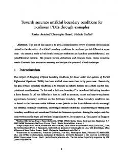
Key Words nonreflecting, absorbing, direct numerical simulation ■ Abstract We review artificial boundary conditions (BCs) for simulation of inflow, outflow, and far-field (radiation) problems, with an emphasis on techniques suitable for compressible turbulent shear flows. BCs based on linearization near the boundary are usually appropriate for inflow and radiation problems. A variety of accurate techniques have been developed for this case, but some robustness and implementation issues remain. At an outflow boundary, the linearized BCs are usually not accurate enough. Various ad hoc models have been proposed for the nonlinear case, including absorbing layers and fringe methods. We discuss these techniques and suggest directions for future modeling efforts.

1. INTRODUCTION Simulating realistic flows often requires that artificial computational boundaries be drawn between a flow region of interest and other flow regions that one hopes to neglect. In some cases the region of interest may extend to infinity; at other times artificial boundaries must be drawn through a flowing fluid. This article discusses the development of these artificial boundary conditions (ABCs) with an emphasis motivated primarily by turbulent shear flows and their sound generation. Even if radiation to the far field is not of interest, acoustic waves play a role in combustion instabilities, receptivity of shear layers, and many other phenomena of interest. Even in the absence of sound, it is always advantageous to minimize computational effort by allowing artificial boundaries to enclose the region of interest as snugly as possible, without damaging the solution. While the article focuses on the unsteady, compressible Euler and Navier-Stokes equations, the techniques are also largely applicable to Large Eddy Simulation (LES) and unsteady Reynolds Averaged Navier-Stokes (U-RANS). When the flow near the boundary can be decomposed into small amplitude fluctuations about a uniform state, then analytical solutions for the exterior problem can be used to derive ABCs. Invariance of the solution to the precise location of domain truncation is then equivalent to requiring that there are no incoming waves at the 0066-4189/04/0115-0315$14.00

315

12 Nov 2003

16:2

316

AR

AR203-FL36-13.tex

AR203-FL36-13.sgm

LaTeX2e(2002/01/18)

P1: IBD

COLONIUS

boundary. The resulting nonreflecting boundary conditions (NRBCs) have been studied for about thirty years. Conceptual issues have been largely solved, although a host of technically challenging extensions and implementation details remain. They are outlined in Section 2; fortunately, there are already several good reviews on this topic (Givoli 1991, Tsynkov 1998, Hagstrom 1999). These references also include important links to the literature in computational electromagnetics and other phenomena governed by linear hyperbolic equations. By contrast, when the flow near the boundary cannot be represented as small amplitude disturbances to a nearly uniform state there is little theory with which to develop NRBCs. Important examples include turbulent shear flows (free and wall-bounded), and internal flows in pipes, nozzles, diffusers, turbomachinery, etc. It is usually impractical to model more than a single component of a larger system, or a relatively short length of a spatially developing flow. Complex interactions between the components or regions and their environment are ignored, often producing unrealistic effects. A classic example is the convectively unstable mixing layer. When truncated, computationally or physically, the mixing layer may exhibit self-excited oscillations due to feedback from downstream (Buell & Huerre 1988). Whether and how one models this feedback, or eliminates it altogether, is a problem-dependent modeling choice. Slowly, this important problem has been recognized and there are now examples of experimental studies that seek to characterize BCs for input to numerical computations. In more complex cases, one can always proceed with approximations developed for the uniform flow, but then the accuracy of the results may not justify the burden of implementing accurate NRBCs. Thus, in practical computations, lower-order accurate BCs are typically used. For better accuracy, they are sometimes combined with sacrificial regions, where the governing equations are modified in a finite region adjacent to the artificial boundary. These regions are called by various names: absorbing layers, fringe regions, buffer zones, sponges, and so on. Some of them have been effective in specific flows, but in general they involve a number of free parameters that must be tuned for new situations. In this article, we explore this gap between the largely mathematical topic of NRBCs and the largely empirical practice in computational fluid dynamics of using relatively crude BCs and ad hoc buffer regions. In particular, we stress that mathematics alone cannot fill this gap–there is an open and substantial modeling problem that is no less challenging, and arguably no less important, than subgrid modeling for turbulence.

2. LINEARIZED BOUNDARY CONDITIONS Most ABCs for compressible flow are based on linearization about relatively uniform ambient conditions (the base flow), as depicted in Figure 1. There is a source region, S, which may be nonlinear and contain bodies, external forces, etc. Outside this region any disturbances produced in S will decay, by geometric attenuation and/or through viscous diffusion, so that far away the flow is of uniform

12 Nov 2003

16:2

AR

AR203-FL36-13.tex

AR203-FL36-13.sgm

LaTeX2e(2002/01/18)

P1: IBD

ARTIFICIAL BOUNDARY CONDITIONS

317

Figure 1 Computational domain for linearized BC (left). At right is a computational domain for a turbulent jet where the artificial boundary intersects the source region.

velocity and thermodynamic properties. At some distance disturbances levels will be small so that nonlinear effects may be neglected (the region labeled L). Of course, there may be a potential flow that is set up by the source region that decays only slowly to the uniform state, but it will eventually vary only slowly compared to any disturbance length scales. The goal is to simulate the entire region L extending to infinity, which requires either stretching the grid (infinitely) or truncating the domain at an artificial boundary (denoted ∂B in the sketch). We discuss the possibility of stretching in Section 5.3. Domain truncation at an artificial boundary goes by various names in the literature: absorbing, nonreflecting, radiation, characteristic, artificial, transparent, and so on. Although these names also sometimes imply different techniques, they share the same goal depicted in Figure 1. For an inviscid, nonheat-conducting calorically perfect gas, the linearized conservation laws for mass, momentum, and energy may be manipulated to obtain decoupled equations for (a) the vorticity fluctuations, in the form of a first-order advection equation, (b) the entropy fluctuations, in the form of a first-order advection equation, and (c) pressure fluctuations, in the form of the second-order (advected) wave equation (Lord Rayleigh 1877). Modes are only coupled to one another by BCs, or, in a successive approximation scheme, to mutual nonlinear interaction (Chu & Kovasznay 1958). NRBCs for the second-order wave equation can be readily derived following methods developed for the wave equation (discussed below) and, almost trivially, for the first-order advection equations, by specifying the values of entropy and vorticity fluctuations wherever the mean velocity points into the computational domain. However, most solution methods do not use vorticity as a primary variable. By contrast, the velocity perturbation usually the variable being solved for in a computation is a superposition of the acoustic and vortical modes. [If viscosity is included in the analysis, then the velocity can also be induced by entropic fluctuations (Chu & Kovasznay 1958).] One could proceed to split (Helmholtz decomposition) the velocity into solenoidal and irrotational components associated with the vorticity and acoustic disturbances, respectively. The compressible vortex method

12 Nov 2003

16:2

318

AR

AR203-FL36-13.tex

AR203-FL36-13.sgm

LaTeX2e(2002/01/18)

P1: IBD

COLONIUS

developed by Eldredge et al. (2002) actually solves the equations in that form. However, the splitting is nonlocal in space and requires solving auxiliary elliptic (Poisson) equations, which is relatively expensive compared to other techniques.

2.1. Decomposition at a Planar Boundary At (locally) planar boundaries, the linearized equations in primitive variables (say, density, velocity, and pressure) can be formally decoupled by taking FourierLaplace transforms. The notation is simplified by taking a two-dimensional flow with a single boundary aligned with the x-direction. [The three-dimensional case (e.g., Hagstrom & Goodrich 2002) is a straightforward extension.] The conservation laws may then be written as: qt + Aqx + (B + vo I ) q y = 0, where

  0 uo 0   A =  0 uo + 1 0  , 0 0 uo − 1

 0 1/2 −1/2   0 , B= 1 0 −1 0 0

(1)



(2)

and where the dependent variables are written in one-dimensional characteristic form, q = (v 0 , u 0 + p 0 , u 0 − p 0 )T . Here (u 0 , v 0 ) are velocity fluctuations, uo = (u o > 0, vo ) is the constant base flow, and p 0 and ρ 0 are pressure and density fluctuations, respectively. Variables are nondimensionalized with a characteristic length scale, ambient density, and sound speed so that ρ0 = 1, p0 = 1/γ , and a0 = 1. Note that ρ 0 is eliminated by working in terms of entropy fluctuations (s 0 = p 0 − ρ 0 ), which are in turn governed by a decoupled, first-order advection equation (for which ABCs follow trivially after the analysis of the remaining system). Proceeding with the transforms (with duals to y and t taken as k and s, respectively) yields ˆ qˆ x = −(s + ivo k)M(z)q,

(3)

where z = ik/(s + ivo k) and M(z) = A−1 (I + z B). Thepeigenvalues of M(z) are λ1 = 1/u o , λ2,3 = (u o ∓ µ)/(u 2o − 1), where µ(z) = 1 − z 2 (1 − u 2o ) and where the standard branch of the square root is used. When µ is real the solutions are propagating waves, where λ1 corresponds to the vorticity wave, and λ2 and λ3 to acoustic waves. The simplest case is when wave fronts are normal to the boundary (k = z = 0), for which the one-dimensional eigenvalues are recovered, namely 1/u o , 1/(u o + 1) and 1/(u o − 1). The next step is to label waves as incoming or outgoing (or equivalently rightgoing or left-going) at a given boundary. For simplicity, we take u 0 > 0; therefore the left boundary represents inflow and the right boundary represents outflow. Clearly, if u o >1 (supersonic), then all the eigenvalues are of one sign and represent incoming waves at the left, outgoing waves at the right. For the left boundary, if 0 < u o < 1, the first two modes (vorticity and one acoustic wave) are right-going and the third is left-going. The appropriate NRBC would specify that incoming

12 Nov 2003

16:2

AR

AR203-FL36-13.tex

AR203-FL36-13.sgm

LaTeX2e(2002/01/18)

P1: IBD


319

wave amplitudes are zero. Not all solutions to Equation 1 are propagating waves (e.g., when µ is imaginary), but for these solutions the terminology right-going and left-going refers to the algebraic labeling of modes from the theory of well posedness Higdon (1986). If the matrix M(z) is at least block diagonalizable (as it is for the Euler equations), then a matrix Q can be found such that: Ã ! Ã ! 3R 0 QR −1 Q= , (4) QMQ = 3 = QL 0 3L where R and L superscripts denote block positive- and negative-definite matrices (for z = 0) corresponding to right- and left-going solutions, respectively, and in the second formula Q is partitioned in the same manner.

2.2. Exact Boundary Conditions Boundary conditions for the equations follow directly from the mode labeling. Exact NRBCs are obtained by setting all incoming wave amplitudes to zero. Q R qˆ = 0

(inflow boundary)

Q L qˆ = 0

(outflow boundary).

(5)

[More generally, we may wish to specify a particular forcing on the right-hand-side of Equation 5 to excite entropic, vortical, and acoustic waves]. Note that if u o = 0, the boundary is called characteristic; this degenerate case requires a separate (but straightforward) treatment. In turbulent shear flows, u o = 0 is not common near the boundaries because there is a small entrainment flow. Detailed expressions for Q R and Q L can be found in Rowley & Colonius (2000) and Hagstrom & Goodrich (2002). Note that Equation 5 really represents a family of BCs, all exact, as block diagonalization of M(z) is not unique. If, for reasons discussed below, ˜ R and Q ˜ L ), then approximations are introduced in Q R and Q L (producing, say, Q reflection coefficients will be of interest. At the left boundary, these will represent the amplitude of right-going waves in terms of left-going waves (and vice versa at the right boundary). Let us form a matrix T(z) containing the eigenvectors of M(z). Then fˆ = T −1 qˆ are the decoupled wave amplitudes. Partitioning into leftand right-going modes gives L fˆ = % L ˆf R

R L fˆ = % R fˆ ,

(6)

L L R R where % L = ( Q˜ T L )−1 Q˜ T R and % R = ( Q˜ T R )−1 Q˜ T L . For the subsonic case, R % is a 1 by 2 matrix that represents the amplitude of left-going acoustic waves in terms of right-going vorticity and acoustic waves and % L is a 2 by 1 matrix of right-going acoustic and vorticity waves, both in terms of left-going acoustic waves. In the discussion below, it is helpful to label these separately:

% L = (ρa − →Ä ρa − →a + )T

% R = (ρÄ→a − ρa + →a − ) ,

(7)

12 Nov 2003

16:2

320

AR

AR203-FL36-13.tex

AR203-FL36-13.sgm

LaTeX2e(2002/01/18)

P1: IBD

COLONIUS

where the symbols Ä, a + , and a − represent the amplitudes of the right-going vorticity and right- and left-going acoustic waves, respectively. An important step in constructing BCs is to check that the BCs are well posed. The theory of well posedness (stability) of linear hyperbolic Partial Differential Equations (PDEs) is well established. The uniform Kreiss condition (see Gustafsson et al. 1995, Higdon 1986, Kreiss 1970) is sufficient for well posedness, but more strict than necessary. All that is required for well posedness is that the reflection matrices be bounded for all z ∈ C (Higdon 1986). Obviously, accuracy of the BCs would dictate that the reflection matrices also be small on the imaginary z axis (where solutions are waves). As was first noted by Giles (1988, 1990), the ˜ L ≈ Q L = T −1 L (i.e., 3 is diagonal) always leads to straightforward choice of Q ill-posedness for the inflow BC. This problem is not serious—all one need do is relax the conditions on Q such that 3 is block diagonal, i.e., that the rows of Q L be orthogonal to T R . This leads to a three-parameter family of inflow BCs discussed in Rowley & Colonius (2000) (but of which only a few have ever been tried). ˜ ≡ Q) is that they are nonlocal The more important issue with exact BCs (i.e., Q and involve a convolution integral p in y (transverse to a planar boundary) and time, due to the presence of µ(z) = 1 − z 2 (1 − u 2o ) in both Q R and Q L . Convolution integrals must be discretized, or further approximations must be made. An analogous situation arises in posing NRBCs for the simple wave equation. Although the equations were developed here for a planar boundary, similar results can be obtained in other coordinate systems. However, as pointed out by Hagstrom (1999), computationally efficient evaluation of the convolution integral depends crucially on scale invariance of the artificial boundary, which is obtained for planar, spherical, cylindrical, and conical domains. Some specific nonlocal techniques for the wave equation are those of Ting & Miksis (1986), who showed that nonlocal BCs can be formulated with the Kirchhoff integral formula (applicable to any smooth boundary shape). Sofronov (1993) and Grote & Keller (1995, 1996) developed implementations for spherical domains (in particular, temporally local conditions in terms of spherical harmonics). For time-harmonic problems, the socalled Dirichlet to Neumann (DtN) BC was developed by Keller & Givoli (1989), and extended to implicitly discretized time-dependent problems (Helmholtz equation) by Givoli (1992). In odd numbers of spatial dimensions, the presence of distinct aft wave fronts limits the extent of temporal nonlocality of the exact BC, which can be exploited in computations (Ting & Miksis 1986, Givoli & Cohen 1995). More recently, Ryaben’kii et al. (2001) developed techniques based on this principle directly for discrete finite-difference (FD) formulations. The extent to which similar nonlocal techniques have been investigated for the linearized Euler equations is limited. For steady flows, the disturbance potentials method (DPM) developed by Ryaben’kii and coworkers utilizes nonlocal boundary operators and offers several attractive implementation features. Tsynkov (1998) discussed these, and good results have been obtained for a number of flow configurations (e.g., Tsynkov et al. 2000). For unsteady flows, Gustafsson’s (1988) early work used approximations to develop a BC that was local in space, but involved

12 Nov 2003

16:2

AR

AR203-FL36-13.tex

AR203-FL36-13.sgm

LaTeX2e(2002/01/18)

P1: IBD


321

integration over time. Recently, Sofronov (1998) proposed a method of evaluating the convolution sums by approximating the convolution kernel by a sum of exponentials. The resulting convolution was then reduced to recurrence formulas applied locally in time. A similar technique Dedner et al. (2001) was implemented in the planar case for the linearized equations of magnetohydrodynamics.

2.3. Local Approximate Boundary Condition If polynomial or rational function approximations for µ(z) are inserted into Equation 5, local differential equations are obtained for a point on the boundary. The computational efficiency of implementing local conditions led early investigators (Lindman 1975; Engquist & Majda 1977, 1979; Bayliss & Turkel 1980) to develop hierarchies (of increasing order-of-accuracy) of local conditions for the wave equation. By now, equally efficient methods have in some cases been devised for the nonlocal operators, as discussed above, but there is still an advantage to localizing the BC: nonuniform base flow can be accommodated by adjusting the quantities p0 , ρ0 , and uo to the local base flow on a point at the boundary, as discussed in the next section. It is perhaps most natural to think of a Taylor series approximation of µ(z) about z = 0, which corresponds to waves striking the boundary at normal incidence– always the case in one spatial dimension. Indeed, the crudest approximation is that z = 0, which specializes Equation 5 to: (v 0 u 0 + p 0 )T = 0

(1D inflow)

u 0 − p0 = 0

(1D outflow).

(8)

In fact, these are just the linearized variables that are constant along characteristics. Their nonlinear counterparts (discussed in Section 4), are widely used in compressible flow computations. Lindman (1975) and Engquist & Majda (1977) considered the wave equation with Padé approximations to µ(z) about z = 0. Trefethen & Halpern (1986) proved a number of important theorems regarding rational approximations to µ(z) ≈ pm (z)/qn (z) (where m and n are the degrees of the numerator and denominator polynomials, respectively) that lead to well-posed BCs. These include all Padé, Chebyshev, and least-squared approximations, provided that m = n or m = n + 2. Thus, Taylor series approximations are not valid for order higher than two. Giles (1988, 1990) derived local BCs for the Euler equations by low-order Taylor series expansions for µ(z). His strongly well-posed BCs have zero reflection coefficients for ρa − →Ä and ρÄ→a − , and acoustic reflections with ρa − →a + = 0(z 4 ) and ρa + →a − = O(z 2 ). Rowley & Colonius (2000) showed that strongly well-posed BCs with arbitrarily high-order accuracy can be obtained under the same conditions on rational function approximations as discussed above for the wave equation. For (m, n) Padé approximants, one again has zero reflection coefficients for ρa − →Ä and ρÄ→a − , but now ρa − →a + = 0(z m+n+4 ) and ρa + →a − = O(z m+n+2 ). These are equivalent to Giles’s conditions when m = n = 0. Hagstrom & Goodrich (2002) developed similar BCs. When higher-order approximations are used for µ(z), the

12 Nov 2003

16:2

322

AR

AR203-FL36-13.tex

AR203-FL36-13.sgm

LaTeX2e(2002/01/18)

P1: IBD

COLONIUS

Figure 2 Reflection coefficients for different linearized NRBC with u o = 0.5. One dimensional (— — —); Linearized Thompson (1987) (– – – –); Modified Giles (1990) (— · —); (0, 0) Padé (also Giles) (¤); (2, 0) Padé (M); (2, 2) Padé ( e); (4, 4) Padé (O).

local BCs are high-order differential equations with mixed partial derivatives in y and t. For discretization, these can be reduced to a system of first-order PDEs, implemented by defining auxiliary variables (Rowley & Colonius 2000, Hagstrom & Goodrich 2002). Figure 2 shows reflection coefficients for various local BCs, for the case when u o = 0.5. They are plotted versus the angle (measured from the x-axis) of the acoustic wave that generates the reflection (or versus the angle of the generated upstream running acoustic wave in the case of the Ä → a − reflection). These angles are unique functions of z. The higher-order Padé approximations give uniformly better results. For example, the (4, 4) Padé gives less than 1% reflection of acoustic waves, making angles smaller than 100◦ to the right boundary and 45◦ to the left boundary. By contrast, similar error levels require less than 20◦ and 5◦ for the one-dimensional BC. A property of all well-posed local BCs is that the reflection coefficient is unity for waves whose group velocity is tangent to the boundary (µ = 0). In flows with periodic (or wall) boundaries transverse to the nonreflecting direction, this leads to relatively poor performance at long times because after a time only tangent waves remain. In aperiodic domains, a more serious problem arises involving implementation of the planar BCs discussed here near edges and corner points of rectangular domains. Ideally, one would derive a set of compatibility conditions that would blend the differing approximations on the intersecting boundaries. However, except for lowest-order conditions stable corner treatments have not been found, although Collino (1993) presented compatibility conditions for the wave equation. One treatment is to write the BCs in terms of derivatives normal to the boundary (using the full governing equations), thus applying the BCs as closures for the derivatives (e.g., Rowley & Colonius 2000). Then at the corner

12 Nov 2003

16:2

AR

AR203-FL36-13.tex

AR203-FL36-13.sgm

LaTeX2e(2002/01/18)

P1: IBD


323

point, one specifies the BC for both derivatives. This approach is similar to one discussed for (nonlinear) characteristic BC in Section 4. While no proof of stability exists, computational experiments imply that this approach is stable for the (0, 0), (2, 0), and (2, 2) conditions. The performance of these cases is discussed in Section 5.1, where they are compared to results using the Perfectly Matched Layer (PML). The corner problem would be obviated by using a smooth (e.g., cylindrical or spherical) boundary and by extending local or nonlocal techniques developed for the wave equation to the linearized Euler equations. However, a new problem arises in that the sign of the base flow velocity would necessarily reverse at a point on the boundary (hence changing the labeling of modes that is the basis of the analysis). Both corner and mixed inflow/outflow boundaries represent important future challenges. Another technique that can be used to localize the exact BC consists of taking an asymptotic expansion of the solution for large distances from the source region (Bayliss & Turkel 1982). For the wave equation, the first term recovers the classical Sommerfeld radiation condition, but applied at a finite distance rather than at infinity. For the linearized Euler equations, Bayliss & Turkel derived conditions suitable for the outflow and characteristic u o = 0 boundaries. Tam & Webb (1993) extended the analysis to inflow boundaries, but only for the first term in the expansion. The one-term expansion suffers inaccuracies whenever the source is not centered within the boundary because the asymptotic expansion converges only slowly in the general case. Hagstrom & Haariharan (2003) have extended the inflow hierarchy for the convected wave equation, and it is likely that full extension to the linearized Euler equations (i.e., inclusion of vortical and entropic modes) is possible.

2.4. Nonuniform Base Flows In principle, the local BC discussed in the last section can be applied to nonuniform base flows by adjusting ρ0 , p0 , and uo that appear in (the dimensional versions of ) the BC to their local values, provided that the variation of the base flow is long compared to the length scale of the disturbances. Although useful in many flows of practical interest, this high-frequency approximation is not accurate at inflow and outflow boundaries of turbulent shear flows, where the largest vortical structures are on the same scale as variation of the base (mean) flow and peak acoustic radiation is at longer wavelengths. Thus, it is unclear that there is anything to be gained by implementing the exact or higher-order approximate BC. In practice, the lowerorder conditions [one-dimensional, Giles (1990), and one-term asymptotic] have been used extensively in computations of mixing layers and jets (e.g., Colonius et al. 1993, Tam & Dong 1996a, Morris et al. 1997, Mitchell et al. 1999, Freund 2001, Bogey & Bailly 2002). Several of these studies combined the lower-order BC with an absorbing buffer region (Section 5) near the outflow boundary. The problem is that acoustic, vortical, and entropic modes lose their distinct identity in the presence of arbitrary mean flow gradients. A few nonuniform base

12 Nov 2003

16:2

324

AR

AR203-FL36-13.tex

AR203-FL36-13.sgm

LaTeX2e(2002/01/18)

P1: IBD

COLONIUS

flows are, or might yet be, analytically approachable. Dedner et al. (2001) derived exact NRBCs for a quiescent base state that was stratified in the direction normal to the boundary. Although unexplored, NRBCs for parallel (unidirectional, transversely sheared) flows may be tractable because it is possible to derive a thirdorder wave equation for the pressure–the same one that is used for linear parallel flow instability. [A recently proposed extension of the PML technique for parallel shear flows by Hagstrom & Nazarov (2002) is discussed in Section 5.1.] Goldstein (1984) reviewed this equation in detail; solutions correspond to the two acoustic waves and an arbitrary advecting gust solution that has nonzero vorticity. There is also a spatially growing instability wave whose pressure decays exponentially fast away from the shear for subsonically convecting waves. As before NRBCs would follow from decoupling left- and right-going solutions and dealing with the nonlocality associated with the acoustic waves and further hydrodynamic pressure fluctations associated with the vortical motion. Although extension to parallel shear flows and other nonuniform flows remains a worthy future challenge, it should at the same time be recognized that for turbulent flows, nonlinear effects discussed in Section 4 may be equally important, especially at the outflow boundary.

3. DISCRETIZATION EFFECTS When ABCs for the continuous (linearized) Euler equations are discretized, new issues and ambiguities arise. I discuss the problem in the context of FD discretization because they are most widely used, but analogous effects can occur in other discretizations. [Hu & Atkins (2003) recently analyzed discrete effects in NRBCs for the Discontinuous Galerkin Method.] Discrete effects are important because if ignored, they can lead to instabilities or degrade the accuracy. The two most obvious (and interrelated) problems are (a) that wide FD stencils cannot be accommodated at the boundary or near-boundary nodes, and (b) that BCs are provided on some (but not all) of the dependent variables. I refer to these as boundary closure problems to distinguish them from the physical problem of posing BCs for the continuous equations. The generic solution to (a) is to combine interior FD schemes with special one-sided and biased schemes for the boundary and near-boundary nodes, respectively. A commonly cited result is that the onesided and biased FD schemes at the boundary can be one order of accuracy lower than the interior scheme such that the the overall scheme has the same formal order of accuracy as the interior (Gustafsson 1975). Problem (b) is usually resolved by one of two methods: by extrapolating unspecified variables from the interior, or by requiring some (or a linear combination) of the full governing equations to be satisfied at the boundary. Obviously, for the latter any derivatives normal to the boundary appearing in those equations will also require one-sided FD schemes. Both procedures can assure accuracy of boundary closures, but stability of the resulting discretized equations requires additional considerations. The stability of the interior FD equations with periodic BC is readily analyzed with Fourier

12 Nov 2003

16:2

AR

AR203-FL36-13.tex

AR203-FL36-13.sgm

LaTeX2e(2002/01/18)

P1: IBD


325

methods (i.e., von Neumann stability analysis), but gives neither necessary nor sufficient conditions for the general case. For first- or second-order-accurate FD schemes, which require special treatment only of the boundary point, this has not posed a serious difficulty. Providing stable closures for high-order, and especially compact FD schemes, has been much more difficult. Most analyses have concentrated on the development of boundary closures that are stable in the context of the one-dimensional linear advection equation: u t + cu x = 0,

x ∈ [0, 1]

u(x, 0) = g(x)

u(0, t) = h(t),

(9)

where c > 0 and there is an inflow boundary at x = 0. As Carpenter et al. (1993) discussed, there are two important types of stability. The first (Lax stability) determines whether the solution remains bounded as the mesh size 1x → 0 at a fixed time, and the second ensures that the error does not grow without bound in time. The G-K-S theory (Gustafsson et al. 1972) shows how Lax stability can be analyzed in terms of normal modes on semi-infinite or finite domains. Requiring that the error does not grow without bound in time requires asymptotic stability, which for the semidiscrete case implies that there can be no eigenvalues of the spatial discretization operator in the right half of the complex plane (or on the imaginary axis in the degenerate case). Carpenter et al. (1994) stressed the desirability of having schemes that are both Lax and asymptotically stable. In the context of Equation 9, it is not difficult to derive boundary closures and check, a posteriori, for stability (e.g., Lele 1992, Hixon 2000). Generally, eigenvalues must be determined numerically, for a specified grid size, but it is straightforward to examine several cases and extrapolate to larger grids. Such analyses show that it becomes difficult to find stable closures unless accuracy is sacrificed at the boundary. Although it is desirable to maintain high accuracy near the boundaries, boundary closures applied to more complex equations are usually combined with other approximations to the continuous BCs such as those discussed in Sections 2 and 5. Given this, the order of accuracy near the boundaries is not as important as stability and related conservation properties. Carpenter et al. (1994), Abarbanel & Chertock (2000), and Abaranel et al. (2000) constructed stable closures (both Lax and asymptotic) for high-order compact FD methods by requiring that the discrete approximation admit a summationby-parts (SBP) formula. The stability requirement is reduced to a set of algebraic constraints on the coefficients of the boundary or near-boundary FD formulas. The method requires that the BC be posed using the simultaneous approximation term (SAT) method, which amounts to enforcing the BC nonlocally in space. This sort of penalty method is similar in spirit to the buffer region techniques that will be pursued in Section 5. Physically, the effect is to add to the equations a dissipative term that drives the solution to the specified BC in a region near the boundary. Abarbanel & Chertock (2000) generalized this approach and proved stability for multidimensional scalar equations and, under certain conditions, systems of one-dimensional equations. Abarbanel et al. (2000) applied their technique to more general equations a posteriori, including the multidimensional Maxwell equations with good

12 Nov 2003

16:2

326

AR

AR203-FL36-13.tex

AR203-FL36-13.sgm

LaTeX2e(2002/01/18)

P1: IBD

COLONIUS

results and no apparent instability. Carpenter et al. (1999) used the SAT/SBP schemes to impose conditions at interfaces between subdomains. Nordström & Carpenter (1999) described generalization to one-dimensional systems of nonlinear viscous and inviscid equations, and finally, application to generalized curvilinear coordinates for multidimensional, scalar, linear hyperbolic equations (Nordström & Carpenter 2001). Further generalization is no doubt possible, and would hopefully include consideration of more accurate BCs for multidimensional flows. A different approach to the boundary closure/stability problem follows from a consideration of the dispersive properties of FD approximations (Trefethen 1982). Vichnevetsky developed nonreflecting BCs that account for discrete, dispersive effects in a series of papers (see Vichnevetsky 1987). He analyzed Equation 9 with a second-order central FD scheme, u x ≈ (u j+1 −u j−1 )/(21x), on an infinite regular grid with spacing 1x. By taking a Fourier transform (in time) of the semi-discrete iωt j ˆ κ to the equations, he found normal-mode solutions by inserting u j (t) = u(ω)e resulting Ordinary Difference Equations. The shift operator, κ ∈ C, is the solution of the dispersion relation: κ 2 + 2iÄκ − 1 = 0, where Ä = ω1x/c. There are, for any given frequency, two solutions: p κ = −iÄ ± 1 − Ä2 ,

(10)

(11)

with constant unit amplitude whenever the frequency is below a cutoff frequency, ωC < c/1x. [Beyond the cutoff frequency, the solutions correspond to waves that are exponentially growing or decaying in x. These can only be excited by forcing the boundary at x = 0 with ω > ωC , which should be avoided.] Their wavenumber is given by arg κ, against which frequency is plotted for each root in Figure 3. The first solution has the correct group velocity, c, for sufficiently small wavenumber. These physical waves correspond, as 1x → 0, to the converged solution to Equation 9. The second solution is characterized by group velocities that are negative and corresponds to poorly resolved waves with only a few points per wavelength. These waves have no physical counterpart and are therefore termed spurious waves. An interesting conclusion is that the spurious waves can create unphysical feedback from downstream, even in a supersonic flow. In the subsonic case, they provide an additional route to feedback beyond (physical) acoustic waves that could be excited by approximations in the continuous outflow BC. Buell & Huerre (1988) and Colonius et al. (1993) have examined how such spurious feedback can lead to self-forcing of (nominally convectively unstable) shear layers. Any centered difference scheme in Equation 9 is dispersive and admits physical and spurious solutions. Larger stencils produce additional spurious modes that are exponentially decaying with distance from the boundary (into the domain). If upwind biased FD schemes are used, the spurious waves are, by virtue of their short wavelength, rapidly damped and usually not a significant feature of the solution. However, DNS and LES more often use low-dissipation and higher-order

12 Nov 2003

16:2

AR

AR203-FL36-13.tex

AR203-FL36-13.sgm

LaTeX2e(2002/01/18)

P1: IBD


327

Figure 3 The normal mode solutions (physical and spurious) to the semidiscrete version of Equation 9 with central second-order FD.

FD schemes (e.g., Mittal & Moin 1997). Although it is desirable to have a wellresolved solution such that spurious waves are minimized, they are nevertheless always present to some degree in nonlinear calculations, particularly in LES. Even though the dispersion analysis allows a host of important issues regarding numerical accuracy to be analyzed (e.g., Trefethen 1982), the issues most relevant here are boundary closures and stability. The continuous BCs of Equation 9 are trivially nonreflecting. However, in the discrete case the normal mode solutions are coupled nonlocally in time, and any local BC or boundary closure will couple the normal modes and there will be reflections–physical to spurious at the outflow boundary and vice versa at the inflow boundary. Following the ideas presented in Section 2, it is clear that boundary closures should be constructed to eliminate or at least minimize these reflections. Elimination would require a closure that is nonlocal in time, but local conditions can be obtained by introducing approximations. Vichnevetsky (1987) derived several local conditions for the second-order FD scheme by taking a Taylor series expansion of the normal mode solutions. Colonius (1997) generalized the treatment and derived conditions compatible with a fourth-order compact FD scheme. Generalization to wider stencils is conceptually straightforward, although the algebra becomes increasingly tedious. These boundary closures are termed discretely nonreflecting to distinguish them from the physically NRBC for continuous equations of Section 2. Importantly, reflection coefficients also determine the stability of the boundary closure. By analogy with the multidimensional case, stability dictates that reflection coefficients be bounded for all ω ∈ C (Trefethen 1983). Boundary closures can also be developed to reduce the reflection of spurious waves at a solid wall (Tam & Dong 1996b, Collis & Lele 1997), where the discrete equations support two types of spurious waves: the short wavelength propagating wave discussed above and a spatially damped wave that is trapped near the wall.

12 Nov 2003

16:2

328

AR

AR203-FL36-13.tex

AR203-FL36-13.sgm

LaTeX2e(2002/01/18)

P1: IBD

COLONIUS

The discretely NRBC developed for the one-dimensional advection equation can be extended to the multidimensional NRBC for the linearized Euler equations (Rowley & Colonius 2000). In the discrete (isentropic) case, there are nine reflection coefficients at any boundary (compared to four for the continuous case), because each physical wave (vorticity and the two acoustic waves) has a spurious counterpart that has opposite group velocity at the boundary. When local approximations to the continuous NRBC are used (such as the Padé approximants), then the equations are only approximately decoupled at the boundaries, and there are two sets of approximations: localization of the continuous exact BC and localization of the discretely exact BC for the one-dimensional advection equation. The errors of one kind can be worsened by making the other kind more accurate. Rowley & Colonius (2000) examined several test cases and chose optimal combinations of Padé approximations and boundary closures. Neither the SBP/SAT or discretely NRBC approaches have yet been used in more general computations, such as those involving nonuniform mean flows, domains with corners, nonlinearity, viscous effects, etc. There is nothing inherent in either approach that would prevent them from being used in an approximate way in more general situations–the most serious question is whether the additional accuracy and stability that they afford is carried over in the presence of (perhaps less accurate) approximations needed in more general cases. Hagstrom (2000) developed an alternative approach to deriving stable closures for FD schemes. He attributes instability associated with boundary closures with the Runge phenomena (large oscillations in interpolating polynomials near the boundaries of evenly spaced grids). He demonstrates that clustering of grid points near boundaries can eliminate instabilities associated with high-order one-sided difference closures. For example, Chebyshev clustering yielded stable schemes but gave rise to undesirable stability constraints. Nodes associated with a recently developed hybrid Gauss-Trapezoidal quadrature scheme (Alpert 1999), which relax to an evenly spaced grid in the interior, give both stability and computational efficiency.

4. NONLINEAR CHARACTERISTIC BC For the case of one-dimensional flow, BCs follow immediately from the classical method of characteristics solution (Hedstrom 1979). That is, it is possible to locally identify and decouple left-going and right-going waves, even in the nonlinear case. Three characteristic curves (in x − t) can be identified whose slopes are λ1 = u, λ2 = u + a, and λ3 = u − a. BCs are required for any characteristic crossing into the computational domain (based on the sign of λ). The integrated values of the dependent variables along the characteristic curves are known as Riemann invariants, and these BCs are usually referred to by that name, or by the term characteristic BCs. When a uniform flow is linearized, these BCs reduce to the one-dimensional approximation given in Equation 8.

12 Nov 2003

16:2

AR

AR203-FL36-13.tex

AR203-FL36-13.sgm

LaTeX2e(2002/01/18)

P1: IBD


329

The BCs discussed above are exact only for one-dimensional problems, but may be used as an approximation in multidimensional flow. Thompson (1987, 1990) proposed a similar BC in the multidimensional case. In his notation, the conservative form of the equations are written qt + P(u)S(u)L + g(q) y = 0,

(12)

where q and g(q) are the standard conserved variables and their fluxes transverse to the boundary, and u = (ρ, u, v, p)T are the primitive variables. P is the Jacobian ∂qi ), matrix that transforms between conservative and primitive variables ( pi j = ∂u j and S is a matrix whose columns are the right eigenvectors of A and L is a vector whose components are L1 = λ1 vx ,

£ ¤ L2 = λ1 s = λ1 px − a 2 ρx , £ ¤ L3 = λ2 u x + (ρa)−1 px , £ ¤ L4 = λ3 u x − (ρa)−1 px .

(13)

These are just the slopes of the characteristic curves multiplied by the x−derivatives of the Riemann invariants. The analysis proceeds identically to the one-dimensional case by specifying the values of L at the boundary when the one-dimensional characteristics are directed into the computational domain (and by using one-sided differences in Equation 13 when they are dircted out). Note that upon linearization, Thompson’s approach is not equivalent to Equation 8 because of the transverse derivatives that are included in Equation 12. Reflection coefficients for linearized Thompson BC are plotted for u o = ao /2 in Figure 2. For ρa + →a − (e.g., at subsonic outflow), these BCs are better than the one-dimensional conditions. For plane acoustic waves transverse to the boundary (which are different from the tangent waves unless u o = 0), the reflection coefficient at the outflow boundary is identically zero. This can be seen by inspection of Equation 13 because all x−derivatives vanish in this case. However, for outgoing vorticity waves the acoustic reflection is larger, and the acoustic reflections at the inflow are larger than for the corresponding one-dimensional conditions. Except when u o = 0, the linearized Thompson BCs are not strongly well posed, as apparent by the presence of infinite reflection coefficients along the inflow boundary. This point corresponds to plane acoustic waves propagating in the transverse direction; because s is purely imaginary for these waves the ill-posedness is weak. In the absence of other sources of dissipation, the computation will be marginally stable. Remarkably, this ill-posedness may actually be advantageous when the BCs are applied near corners and edges of a fully aperiodic domain, which is a serious problem for the BCs of Section 2.3. In this case, any plane wave in the transverse direction is perfectly absorbed by the transverse boundary. At the corner, the conditions are compatible—one simply imposes BCs simultaneously on L and the equivalent transformation of the y-fluxes. In tests and in practical

12 Nov 2003

16:2

330

AR

AR203-FL36-13.tex

AR203-FL36-13.sgm

LaTeX2e(2002/01/18)

P1: IBD

COLONIUS

computations, this appears to be robust, though the errors near the corner are large (e.g., Thompson 1990, Poinsot & Lele 1992). Returning to the nonlinear case, although the BCs discussed share similarities with the linearized BCs of Section 2, there are fundamental differences. The incoming characteristics must carry information about the entire flow—not just disturbances to a base state—into the computational domain. Even labeling of L as incoming or outgoing is a dynamic process that could change signs on a given boundary or in time. In rare cases, a complete solution of the Euler equations in the exterior could be used to compute L. Usually, L must be specified based on minimal information about the exterior problem. For the inflow, one might wish to impose a target velocity profile, as well as perhaps temperature or another thermodynamic variable. The traditional approach is to simply impose Dirichlet BCs on the correct number of variables—four in the case of inviscid subsonic inflow (in three dimensions). Such BCs have been studied extensively and proofs of well posedness exist for a number of different specifications, often for both inviscid and viscous cases. Poinsot & Lele (1992) described a method that combines Dirichelt BCs for velocity and temperature and Thompson-style analysis for the remaining L needed to close the continuity equation. The problem is that all the Dirichlet BCs are badly reflective for the upstream propagating acoustic wave, forcing fluctuations in certain acoustic variables to zero. Upon linearization, imposing the one-dimensional characteristics will be equivalent to the one-dimensional NRBC and therefore at least transparent to plane waves propagating upstream, but imposing velocities and density perturbations to zero will be perfectly reflecting even for plane waves. However, a much less reflective inflow can be constructed if more is specified about the incoming flow. Sometimes the inflow will be laminar with small disturbances, and linearization is appropriate, i.e., L = Lo + L0 . In the inviscid case, steady, unidirectional, transversely sheared flows are an exact solution, provided pressure is constant. Linearizing about this state, Lo = 0 and all incoming L0 should be specified. For the viscous case, often a solution of the boundary-layer equations is appropriate, and in this case Lo depends on the (slow) variation of boundary-layer thickness with the streamwise coordinate. In principle, any BCs discussed in Section 2 could then be used to specify conditions for L0 , but with the caveats discussed there. At a subsonic outflow, one BC is required in the inviscid case. In three dimensions, the other four variables can be found from Thompson’s approach, as in the inflow case, or equivalently Poinsot & Lele’s locally one-dimensional, inviscid (LODI) approach. The problem is to specify the sole incoming characteristic, L4 . If linearization about a uniform state is appropriate (it seldom is at the outflow), then NRBCs for L04 (discussed in Section 2.3) should be used. For linearized Thompson conditions, this would become L04 = 0, with reflectivity of nonplanar waves as shown in Figure 2. However, in the majority of situations, fluctuations about the mean flow are not small, and the mean flow is not known anyway. [Morris

12 Nov 2003

16:2

AR

AR203-FL36-13.tex

AR203-FL36-13.sgm

LaTeX2e(2002/01/18)

P1: IBD


331

et al. (1997) proposed that a steady RANS solution be used for the mean flow, but nonlinearity still prevents very accurate NRBCs from being achieved.] Errors due to nonlinearity at the outflow boundary can be assessed in certain simple model problems. For example, Colonius et al. (1993) considered the propagation of a zero-circulation vortex through the outflow boundary in an otherwise uniform flow. The solution (close to exact for small viscosity) is that the vortex propagates with constant speed, unaltered by the uniform flow. Colonius (1993) and Colonius & Ran (2002) considered two lineraized BCs for this problem: the Giles (1990) outflow condition presented in Section 2.3, where in the linear case outgoing vorticity produces no incoming acoustic wave, and the modified Giles condition, which produces incoming acoustic waves proportional to the amplitude of the vortex. The results, shown in Figure 4, demonstrate that when the induced velocity from the vortex is a significant fraction of the uniform velocity, nonlinear reflections are as significant as linear reflections from the less-accurate BC. Adding shear at the boundary would likely make matters worse. In this example, it is even possible for the sign of λ1 to change as a function of time (changing outflow to inflow) when the strength of the vortex is large enough. This condition causes the linearized treatment to fail. However, even in less pathological cases, nonlinearity produces large reflections. Here, the extent to which imposition of ABC is really a modeling exercise is apparent—analysis alone cannot provide the missing information needed to specify the incoming wave. Because they offer greater flexibility in modeling, some of the buffer techniques described in Section 5 are presently the most accurate

Figure 4 Performance of linearized outflow BC for propagation of a nonlinear vortex (characterized by its maximum induced velocity, Vmax ) in a uniform flow, u o . The 0 maximum normal velocity in the acoustic reflection, vmax is plotted. The Giles condition would, in linear calculation, produce no reflection. For reference, the supergrid model (see Section 5) is also plotted. Giles (1990) (•); Modified Giles ( ¥ ); Colonius & Ran (2002) supergrid (N).

12 Nov 2003

16:2

332

AR

AR203-FL36-13.tex

AR203-FL36-13.sgm

LaTeX2e(2002/01/18)

P1: IBD

COLONIUS

techniques for outflow boundaries. However, I mention here some characteristicbased techniques because they remain widely used. For nonlinear calculations, Thompson (1990) suggested the use of L4 = 0, but this is problematic because there is nothing to prevent the time-averaged pressure from drifting, especially if characteristic BCs are also imposed at the inflow (Rudy & Strikwerda 1980, Poinsot & Lele 1992). On physical grounds, the upstream propagating characteristic would provide whatever acoustic reflections were needed to fix the downstream pressure, at least under steady conditions. Of course, using a simple Dirichlet condition p = p∞ would rectify this [as indeed is still standard practice in many Computational Fluid Dynamics (CFD) codes], but this corresponds to a badly reflective boundary —perfectly reflective for plane waves. Rudy & Strikwerda (1980) proposed the use of a modified version of the one-dimensional characteristic condition pt − ρau t + α ( p − p∞ ) = 0

(14)

that modifies the reflectivity of the boundary so that, at steady state, the pressure there is imposed. α is an adjustable parameter that was optimized to achieve steady state most rapidly in a one-dimensional, linearized problem. It was later used by Poinsot & Lele (1992) in the characteristic formulation, and by Colonius et al. (1993) in implementing Giles conditions in sheared flows. Unfortunately, there has been no systematic study on how to prescribe α in general. The required value is likely dependent on a number of factors, including discrete stability issues discussed in Section 3. Because the one-dimensional characteristic ABCs of Thompson (1987) and Poinsot & Lele (1992) have proven robust in practice, they have been widely used in compressible flow simulations, and some useful extensions have been made. Thompson (1990) uses the same framework discussed above for inflow/outflow boundaries to enforce conditions for walls (inviscid and no-slip), constant pressure, and a force-free BC. The latter sets to zero all forces acting on the fluid normal to the boundary, and the fluid element is advected at the fluid velocity (similar in spirit to the often-used convective BC in incompressible flow). Poinsot & Lele (1992) offer similar generalizations of their LODI approach for these cases. Okong’o & Bellan (2002) extended the analysis for perfect gases to mixtures of real gases, and Kim & Lee (2000) describe techniques for implementing characteristic ABCs in generalized coordinates. For viscous flows, the required number of inflow and outflow BCs differs from the inviscid case (Strikwerda 1977, Oliger & Sundstrom 1978); additional constraints (beyond the inviscid ones) typically take the form of requiring certain gradients of the dependent variables (or combinations of them) to be zero at the boundaries. For the most part, formulations to date have focused on (a) obtaining a well-posed problem in the continuous case and a stable problem in the discrete case, and (b) avoiding the creation of viscous boundary layers at inflow and outflow boundaries by requiring that the inviscid BCs are obtained (smoothly) in the limit as viscosity vanishes (e.g., Dutt 1988).

12 Nov 2003

16:2

AR

AR203-FL36-13.tex

AR203-FL36-13.sgm

LaTeX2e(2002/01/18)

P1: IBD


333

Well posedness is a necessary goal, but unfortunately nonreflectivity of the viscous ABC has been limited to one-dimensional analysis, even in the linearized case. Nordström (1995) showed that when the flow near the boundary can be linearized about a uniform state, then one-dimensional NRBCs (which recover the inviscid conditions in the limit of Re → ∞) can be found that are strongly well posed for the continuous problem and strongly stable in discrete approximations to it. The BCs so derived have the interesting feature that they are maximally dissipative. This means that, in the absence of forcing at the boundary, the energy (norm) will be driven down more rapidly than any other (one-dimensional) BC of the general form considered there. Hasthaven & Gottlieb (1996) took a similar approach, discussing their implementation in a spectral collocation framework. Other work on viscous BCs demonstrates the complex interaction between continuous BCs and closures for FD schemes near the boundary. For example, many practitioners simply use inviscid BCs (usually characteristic-based) with no additional constraints beyond using one-sided differences to close the viscous derivatives. This is probably only justified at a high Reynolds number. Some studies (both theoretical and empirical) have examined the effects of extrapolating all flow variables (or fluxes) at an outflow boundary (Papanastasiou et al. 1992, Nordström 1995, Renardy 1997, Nordström 1999), corresponding to no BC for the continuous case. Of course, the needed closure of the discretization at the boundary (i.e., the extrapolation) does correspond to some BCs, even if it is difficult in general to establish the continuous counterpart.

5. ABSORBING LAYERS As Section 4 discusses, there are significant problems with treating the outflow boundary in turbulent flow where nonlinear effects cause large errors in linearized BCs. In this section, I discuss techniques primarily with this problem in mind— so called absorbing layers where the flow physics are modified in a finite region upstream of the boundary. In many cases the modifications may also be used at inflow and free-field boundaries. Several absorbing layers have been suggested to (a) enhance the efficacy of an ABC or, (b) to obviate the need for any ABC. Many of the essential ideas discussed were introduced by Israeli & Orszag (1981) in the context of linear wave equations. At that time, the techniques they developed were motivated by difficulties in specification of local, NRBCs, even in linearized problems. For linear systems, all of the motivating issues have now been resolved in other ways (see Section 2), but the ideas have inspired a number of techniques that remain widely used in both linear and nonlinear computations. Absorbing layer treatments typically provide for damping of disturbances prior to interaction with an ABC. Some obvious ways to do this are to introduce artificial dissipation (by upwinding), to increase the value of physical viscosity (or add hyperviscosity), and perhaps most simply, to add a linear friction coefficient to the

12 Nov 2003

16:2

334

AR

AR203-FL36-13.tex

AR203-FL36-13.sgm

LaTeX2e(2002/01/18)

P1: IBD

COLONIUS

governing equations qt + N (q) = −σ (x) (q − qo ) ,

(15)

where q is the vector of dependent variables, N(q) is a possibly nonlinear operator, σ (x) is a spatially varying friction coefficient, and qo is some nominal state (zero if the equations are linear) about which disturbances are defined. In most cases σ will blend smoothly between zero in the physical domain and a positive value in the layer. Provided σ is made large enough, then disturbances there are exponentially damped during their residence in the layer. Whatever disturbances are reflected by the boundary are returned but similarly damped as they propagate back through the layer before reaching the domain as reflection error. The basic problem with this approach is that the internal boundary of the absorbing layer (or the region over which σ (x) gradually varies), is itself reflective (Israeli & Orszag 1981); without further modification, the only way to obtain a satisfactory result is to gradually increase the damping from zero over a relatively long distance. This results in thick, computationally inefficient layers.

5.1. Perfectly Matched Layer A way to make the buffer layer nonreflecting is to ensure that the eigenfunctions of the modes of the interior equations are unmodified (except that their phase speed becomes complex such that they are damped), a concept that can only strictly apply to the linearized system. The PML accomplishes this and provides damping of all disturbances within the layer. At the outer edge of the layer, a low-order accurate NRBC (usually one-dimensional characteristic) is posed. PML was first formulated for electromagnetic radiation problems (Berenger 1994) and extended to the linearized Euler equations by Hu (1996). The construction of PML follows closely the modal analysis of Section 2. Early problems with the PML approach included observations of long-time stabilities (Tam et al. 1998, Abarbanel & Gottlieb 1997), but more recent work has resolved these difficulties, and strongly well-posed layers can now be obtained for inviscid disturbances to a uniform mean flow (Abarbanel et al. 1999, Hu 2001, Hagstrom 2003). Unlike the hierarchy of local BCs discussed in Section 2.3, in general there are parameters that must be tuned to optimize the performance of PML. These include the layer thickness (or equivalently number of grid points sacrificed in the layer), and a profile that controls the amount of absorption over the layer, σ (x). Unless the inner edge is treated as an internal boundary (e.g., by characteristic matching, Hagstrom 2003), then the absorption profile should be smooth to the same order as the discretization scheme to avoid spurious numerical reflections. For example, Abarbanel et al. (1999) used σ (x) = C(|x − L|/δ)n , where L is the domain width in x, δ is the layer width, n = 4 is the continuity of the layer (the method used is fourth-order-accurate), and C is a constant strength. In tests involving propagation of two-dimensional acoustic and vorticity pulses in a uniform flow with M = 0.5 (aligned with x) and with C = 1, Abarbanel et al.

12 Nov 2003

16:2

AR

AR203-FL36-13.tex

AR203-FL36-13.sgm

LaTeX2e(2002/01/18)

P1: IBD


335

Figure 5 The error over time due to several different boundary conditions for an acoustic pulse in uniform flow at M = 0.5. The Padé BCs refer to the linearized BCs discussed in Section 2.3. PML refers to the implementation of Abarbanel et al. (1999). Supergrid refers to the absorbing layer in Colonius & Ran (2002). In both cases, N refers to the number of grid points across the layer. For implementation and computational details, see Colonius & Ran (2002).

(1999) demonstrated better accuracy than one-dimensional characteristic BCs with layers as thin as 6 grid points; dramatically better performance (but with greater cost) is obtained with 20 to 30 point layers. Figure 5 shows similar results, where the local (0, 0) and (2, 2) Padé BC (see Section 2.3 and Rowley & Colonius 2000) and the supergrid model (discussed later) are also tested. For the Padé conditions, the ad hoc corner treatment discussed in Section 2.3 was used. The acoustic pulse is tested separately from any vortical disturbance: the local Padé BCs are exactly nonreflecting to linearized vortical disturbances as shown in Figure 4. Error is calculated by computing a reference solution on a much larger domain so that, at the longest times considered, there is inadequate time for any reflection from the boundary. This also allows errors from the BC to be isolated from any other discretization errors. Figure 5 shows that thick PML layers are required to obtain errors comparably small as the (0, 0) Padé BC. The (2, 2) Padé BC gives the best results for short times, but comparable error to the (0, 0) Padé approximation at longer times where the error is due to waves that are tangent to the boundaries (for which all of the local BCs produce unitary reflection coefficients). The higherorder local Padé conditions cannot be compared for this test because of the lack of any stable corner treatment. Hagstrom & Nazarov (2002) extended the PML analysis to nonuniform flows, and in particular parallel shear flows. They showed that although the reflectionless interface between the interior domain and the layer can be maintained, there is no longer any straightforward way to ensure that all waves are damped in the layer. The difficulty stems from physical instabilities associated with the mean velocity profile, although it is shown that by optimization of the free parameters (there are now two, in addition to the layer thickness) satisfactory results were obtained. Further investigation of the method appears warranted, and comparisons with lower-order-accurate BCs that have previously been used in sheared flows (see Section 2.4) should be made.

12 Nov 2003

16:2

336

AR

AR203-FL36-13.tex

AR203-FL36-13.sgm

LaTeX2e(2002/01/18)

P1: IBD

COLONIUS

5.2. Other Absorbing Layers Returning to nonlinear problems, one can anticipate that application of the linearized PML to nonlinear equations will produce the same type of quadratic error (resulting in reflectivity of the interface) as application of linearized, local, approximate NRBCs. For this reason, one might question whether the additional effort of designing nonreflectivity of the layer is justified. Indeed, Freund (1997) showed that some relatively simple modifications of Equation 15 provide reasonable results in the nonlinear case, but with thicker layers than could be achieved in the linearized case. An improvement follows from the observation (Israeli & Orszag 1981) that as the quality of the ABC closing the layer improves, the layer performance improves (to the extent that if the ABC is exact then no absorbing layer is required!). One case for which exact ABC are available (at least for the inviscid case and ignoring discrete effects) is supersonic flow, where at the inflow all modes are incoming, and at the outflow all modes are outgoing. Following Ta’asan & Nark (1995), an artificial convection term may be added to the equations to cause the flow to be supersonic in a layer near the inflow and outflow boundaries. In the outflow case, any waves that are not reflected by the internal boundary of the layer will not produce reflections at the outer boundary. Waves that are reflected are partly damped by the linear friction coefficient in Equation 15 before returning to the domain. Provided the damping and convection are applied smoothly, reflections can be made small. At the inflow boundary, the friction coefficient need not be as large because waves traveling upstream are decelerated to zero speed at the sonic point, and thus their residence time in the buffer is long. An additional benefit is that vortical forcing at the inflow is less damped (with the same value of σ ) because the residence time for incoming disturbances is shorter. A similar approach is that of Karni (1996), where in addition to damping of waves in the layer, the convection speeds are modified by “slowing-down operators.” The concept is to allow for long residence times in the layer so that damping is effective. Karni’s approach is also similar to PML in that he attempts to create layers that are nonreflecting by applying the operators only to the outgoing waves. However, the nonreflectivity in this case is only approximate: the decomposition (of the linearized problem) into modes is one-dimensional, but applied at a specified angle to the boundary that is computed locally based on information from the interior solution. As in PML, the effectiveness of these ad hoc absorbing layers is strongly dependent on the width of the layer. However, they involve an even greater number of parameters and profiles than PML that must be determined empirically.

5.3. Grid Stretching Why not avoid posing an ABC by simply applying a coordinate transformation that would map an infinite domain to a finite one (which could be closed by specifying any fluctuations to vanish)? For PDE with smooth (i.e., nonradiating/advecting) solutions, such a technique is prevalent and accurate, provided some care is taken in

12 Nov 2003

16:2

AR

AR203-FL36-13.tex

AR203-FL36-13.sgm

LaTeX2e(2002/01/18)

P1: IBD


337

choosing an appropriate mapping. However, for radiating/advecting flows, waves with fixed or slowly varying wavelength propagate into the region of mesh stretching, where they become progressively more poorly resolved until they are no longer supported by the discretization. If no further modification is made, then they will be aliased (returned to the domain) in a process that differs depending on the discretization. As discussed in Section 3, FD approximations are dispersive and the most poorly resolved waves attain a negative group velocity. If the grid stretching is infinite, then all disturbances will return, and infinity is thus perfectly reflecting! However, provided that the poorly resolved disturbances are dissipated, either through dealiasing, artificial viscosity, or an explicit damping or filtering operator, then the dispersion associated with grid stretching can actually be an advantage because the residence time in the region of grid stretching can be made indefinitely long by providing more gradual stretching. In other words, the stretching acts in a manner identical to the slowing-down operator of Karni (1996). This is hardly surprising if one considers the effect of grid stretching, say, in a one-dimensional system of (inviscid) conservation laws qt + ξx f (q)ξ = 0,

(16)

where x is the physical coordinate extending to infinity and ξ is the finite computational coordinate. The Jacobian metric ξx will go to zero as x → ∞ and to a constant value (say, unity) in the near-field. If ξ is reinterpreted as the physical coordinate, then the effect is to reduce the convection speed of all disturbances to zero over the region where ξx varies. Rai & Moin (1991) proposed combined grid stretching and filtering as an absorbing layer for incompressible flows and the technique was applied to compressible aeroacoustic problems by Colonius et al. (1993). In both cases, the grid stretching was not infinite—the grid was stretched to a large distance and then terminated with an ABC. In the latter work, explicit filtering of the equations was applied, but with variable coefficients so that filtering was gradually switched on only in the absorbing layer. It was shown that reflections from (nonlinear) vortical structures at the outflow could be reduced by several orders of magnitude compared to the linearized Giles (1990) outflow condition. However, the absorbing layer was quite wide compared to PML. As with the other ad hoc absorbing layers, grid stretching and filtering involve several parameters and profiles that can only be determined through trial and error.

5.4. Fringe Methods, Windowing, and Supergrid Model In the fringe method developed by Spalart (1988) for spatially evolving boundary layers and widely applied thereafter, the need for any inflow and outflow ABC is obviated by using periodic BCs and an absorbing layer to modify the flow near the boundary before it is recycled back as inflow. A linear friction coefficient analogous to that in Equation 15 is added to the right-hand-side of the momentum

12 Nov 2003

16:2

338

AR

AR203-FL36-13.tex

AR203-FL36-13.sgm

LaTeX2e(2002/01/18)

P1: IBD

COLONIUS

equations. The difficulty is in specifying the appropriate qo . It is suggested that the streamwise velocity be driven to a solution of the Navier-Stokes equations (for example, a two-dimensional laminar boundary-layer solution), and made periodic by choosing ¶ µ ¡ ¢ x −L +1 , (17) qo = Q(x, y) − Q(x − L , y) − Q(x, y) S 1 where q now denotes only the streamwise velocity, Q(x, y) is the (approximate) laminar solution, and S(x) is a smoothed step function that varies between zero at the start of the buffer (at x = L − 1) and unity at the edge of the periodic box (at x = L). In using a Fourier spectral method, it is important to ensure that blending functions preserve both periodicity and continuous differentiability, to machine roundoff. Combinations of Gaussian or hyperbolic tangent functions are typically used. The transverse component of velocity should be specified so that the target velocity is divergence free (in the incompressible case). Nordström et al. (1999) recently analyzed the fringe method in detail. By carefully choosing linear, constant coefficient model equations, they argue (and confirm a posteriori with numerical experiments of the full problem) that the periodic fringe method converges (at least in incompressible flow) to the inflow/outflow problem. Specifically, they show that disturbances are appropriately damped prior to recycling at the inflow, and that the upstream influence of the fringe is small. A different approach to using periodic BCs with an absorbing layer is the spatial windowing of the equations proposed in Guo et al. (1994) and revisited recently by Schlatter et al. (2003). Here the governing equations are windowed: w(x)qt + w(x) f (q)x = 0

or q˜ t + (w(x) f (q))x = w0 (x) f (q),

(18)

where the one-dimensional case is written here for simplicity. Here w(x) is the window function, which is zero at the edges of the domain, rises to unity over the fringe, and is unity in the interior. q˜ = w(x)q are windowed variables. Provided that the window function meets certain differentiability and periodicity constraints (Guo et al. 1994), similar to those on S(x), then a Fourier spectral expansion for q˜ is appropriate and spectral accuracy is retained. In general, q cannot be exactly recovered from q˜ because w(x) = 0 at the boundary. In the special case when the desired flow near the boundaries consists of a uniform base flow plus perturbations, a regularized dewindowing operation was ˜ for which Equation 18 can be written as suggested: q ≈ q, ˜ x = 0, q˜ t + w(x) f (q)

(19)

which is exactly analogous to an infinite grid stretching. This also clarifies that disturbances will need to be dissipated as they interact with the fringe so that they are not ultimately aliased back into the interior. As the BC is now periodic, dealiasing is an option, although Colonius & Ran (2002) found that providing an

12 Nov 2003

16:2

AR

AR203-FL36-13.tex

AR203-FL36-13.sgm

LaTeX2e(2002/01/18)

P1: IBD


339

additional absorption of disturbances in the fringe is much more effective than dealiasing alone. For example, Guo et al. (1994) suggest adding a linear friction coefficient term (Equation 15) in the fringe. When it is desired to have some specified inflow velocity profile, then the dewindowing operation needs to be ˜ where qo modified; Schlatter et al. (2003) suggest using q ≈ (1 − w(x))qo + q, would be as specified for the fringe method, Equation 17. In fact, there is a strong analogy between modeling the effect of windowing with the traditional turbulence modeling problem (Colonius & Ran 2002). In turbulence modeling, the concern is with disturbances that become too fine to be represented on the mesh in physical space as the result of nonlinear processes. It is well known that dealiasing (i.e., by using the Galerkin method or by explicit dealiasing of the nonlinear terms) allows this energy transferred to small scales to be removed from the computation, but in a process that is not usually a good model for the true energy cascade. For example, in LES the governing equations are filtered, and a subgrid model is supplied, in essence, to recover the unfiltered variables (needed in the nonlinear terms) from the filtered ones. Filtering in physical space corresponds to windowing in Fourier-space, and vice versa. By windowing, scales that are larger than the extent of the domain are filtered. Thus, by analogy with LES, one should also supply a supergrid model to correct for the unphysical effects of domain truncation. One way to do this would be to develop a more sophisticated dewindowing procedure (e.g., Schlatter et al. 2003). A different approach adopted by Colonius & Ran (2002) is to use q ≈ q˜ and then filter Equation 19 in physical space (a step that is necessary for LES). This is tantamount to dewindowing because by analogy with grid stretching and slowingdown operators, large scales are continuously shortened as they propagate into the fringe. Once filtered, one is presented with the standard LES modeling for the nonlinear products in f(q), as well as additional products of the window function and the fluxes. For the latter, Gaussian filtering and the tensor diffusivity model (Leonard 1974, Leonard & Winckelmans 1999) were chosen. Some additional modifications were needed to ensure that the model is globally diffusive. Results from model problems show good transparency of the boundary using the supergrid model. Figures 4 and 5 compare the performance with other ABCs for propagation of a nonlinear vortex in uniform flow and radiation of an acoustic pulse in free-space, respectively. For the acoustic pulse, the performance is, for an equivalent number of points in the layer (and hence comparable cost) a little better than PML. For the nonlinear vortex, a 10-point layer gives reflections that are 1000 times weaker than the vortex, regardless of the vortex strength, even when the vortex is sufficiently strong to induce inflow at the outflow boundary. Colonius & Ran (2002) presented additional tests and comparisons. One can certainly argue that there is no reason, at this stage, to prefer the windowing/supergrid models to other ad hoc absorbing layers discussed above. The performance is good, but roughly equivalent to what could be obtained by optimizing the parameters and profiles in other treatments. On the other hand, the supergrid model has fewer tunable parameters than other models (Colonius &

12 Nov 2003

16:2

340

AR

AR203-FL36-13.tex

AR203-FL36-13.sgm

LaTeX2e(2002/01/18)

P1: IBD

COLONIUS

Ran 2002). One can reduce the problem to two scalar parameters. The first is the number of points across the layer, the second is maximum slope of the windowing function, w(x), across the fringe. Properly scaled, there is only a small range of values that can be chosen for the slope, and the results are not particularly sensitive to the choice. Aside from requiring fewer tunable parameters, the analogy with turbulence modeling may provide a needed framework in which other (better?) models can be used. Another possible advantage is that the use of periodic BCs may allow energy estimates to be more readily obtained (e.g., Nordström et al. 1999).

6. SUMMARY Techniques for posing artificial (inflow/outflow and radiation) BCs for compressible flows have been studied for many years. For linear problems, or for problems where linearization near the boundary is a good approximation, mathematical analysis of the problem exterior to the domain provide a means to derive ABCs. By and large, theoretical issues have been solved, and a variety of techniques, both local and nonlocal, have been developed that can provide accuracy and stability. However, there are a few stubborn problems that require further investigation: the presence of large gradients in the base flow, compatibility conditions at corners (two-dimensional) and edges (three-dimensional) of Cartesian domains, and locations on boundaries where the sign of velocity changes or where sonic conditions occur. In all cases, there is also a subtle but important interplay between ABCs for the continuous problem and closures used near boundaries in discrete approximations. Discretized equations have more degrees of freedom, and there can be reflections of additional, spurious modes at the boundaries. There is, of course, a strong linkage to the problem of well posedness of the continuous problem, on one hand, and stability of the discrete approximation on the other. In situations where there are significant nonlinear effects near the boundary, primarily the turbulent outflow problem, there is little theory to guide the development of ABCs. In the past, relatively crude ABCs (i.e., one-dimensional characteristic BCs) were typically used, but in recent years improvements to accuracy have been obtained by using ad hoc, but effective, absorbing layers adjacent to the boundary. A variety of specific techniques were discussed, and all of them require several tunable parameters and blending functions that have only been optimized by trial and error. This is not surprising if one recognizes that there is a very close analogy between subgrid scale turbulence modeling and the imposition of ABCs. One deals with scales that are too small to be represented on the discrete mesh, the other with scales that are too large. Some recent models try to exploit this connection by developing windowing techniques that are the largescale analog of the filtering of small scales. However, there is a strong need for new and creative approaches to tackle this important and largely unexplored modeling problem.

12 Nov 2003

16:2

AR

AR203-FL36-13.tex

AR203-FL36-13.sgm

LaTeX2e(2002/01/18)

P1: IBD


341

ACKNOWLEDGMENTS I would like to thank Dr. Jeff Eldredge and Prof. Tom Hagstrom for their helpful comments on a draft of this paper. Much of it was written while I was on sabbatical at Cambridge University, and I am grateful to many colleagues there, particularly Prof. Ann Dowling, for their collaboration and hospitality during my visit. The Annual Review of Fluid Mechanics is online at http://fluid.annualreviews.org

LITERATURE CITED Abarbanel S, Gottlieb D. 1997. A mathematical analysis of the PML method. J. Comput. Phys. 134:357–63 Abarbanel S, Gottlieb D, Hesthaven JS. 1999. Well-posed perfectly matched layers for advective acoustics. J. Comput. Phys. 154(2): 266–83 Abarbanel SS, Chertock AE. 2000. Strict stability of high-order compact implicit finitedifference schemes: The role of boundary conditions for hyperbolic PDEs, I. J. Comput. Phys. 160(1):42–66 Abarbanel SS, Chertock AE, Yefet A. 2000. Strict stability of high-order compact implicit finite-difference schemes: The role of boundary conditions for hyperbolic PDEs, II. J. Comput. Phys. 160(1):67–87 Alpert B. 1999. Hybrid Gauss-trapezoidal rules. SIAM J. Sci. Comp. 20:1551–84 Bayliss A, Turkel E. 1980. Radiation boundary conditions for wave-like equations. Comm. Pure Appl. Math. 33:707–25 Bayliss A, Turkel E. 1982. Far field boundary conditions for compressible flows. J. Comput. Phys. 48:182–99 Berenger JP. 1994. A perfectly matched layer for the absorption of electromagnetic waves. J. Comput. Phys. 114:185–200 Bogey C, Bailly C. 2002. Three-dimensional non-reflective boundary conditions for acoustic simulations: far field formulation and validation test cases. Acustica 88:463– 71 Buell JC, Huerre P. 1988. Inflow/outflow boundary conditions and global dynamics

of spatial mixing layers. In Proc. 2nd Summer Prog., pp. 19–27. Stanford, CA: Stanford Univ. Cent. Turbul. Res. Carpenter MH, Gottlieb D, Abarbanel S. 1993. The stability of numerical boundary treatments for compact high-order finitedifference schemes. J. Comput. Phys. 108(2): 272–95 Carpenter MH, Gottlieb D, Abarbanel S. 1994. Time-stable boundary-conditions for finite-difference schemes solving hyperbolic systems–methodology and application to high-order compact schemes. J. Comput. Phys. 111(2):220–36 Carpenter MH, Nordström J, Gottlieb D. 1999. A stable and conservative interface treatment of arbitrary spatial accuracy. J. Comput. Phys. 148:341–65 Chu BT, Kovásznay LSG. 1958. Non-linear interactions in a viscous heat-conducting compressible gas. J. Fluid Mech. 3:494–514 Collino F. 1993. High order absorbing boundary conditions for wave propagation models, straight line boundary and corner cases. Proc. 2nd Int. Conf. Math. Numer. Asp. Wave Propag. Phenom., pp. 161–71. SIAM Collis SC, Lele SK. 1997. A computational investigation of receptivity in high-speed flow near a swept leading edge. Tech. Rep. TF-71, Stanford, CA: Stanford Univ. Dept. Mech. Eng. Colonius T. 1997. Numerically nonreflecting boundary and interface conditions for compressible flow and aeroacoustic computations. AIAA J. 35(7):1126–33

12 Nov 2003

16:2

342

AR

AR203-FL36-13.tex

AR203-FL36-13.sgm

LaTeX2e(2002/01/18)

P1: IBD

COLONIUS

Colonius T, Lele SK, Moin P. 1993. Boundary conditions for direct computation of aerodynamic sound generation. AIAA J. 31(9):1574–82 Colonius T, Lele SK, Moin P. 1997. Sound generation in a mixing layer. J. Fluid Mech. 330:375–409 Colonius T, Ran H. 2002. A super-grid-scale model for simulating compressible flow on unbounded domains. J. Comput. Phys. 182 (1):191–212 Dedner A, Kröner D, Sofronov IL, Wesenberg M. 2001. Transparent boundary conditions for MHD simulations in stratified atmospheres. J. Comput. Phys. 171:448–478 Dutt P. 1988. Stable boundary conditions and difference schemes for Navier-Stokes equations. SIAM J. Numer. Anal. 25(2):245–67 Eldredge JD, Colonius T, Leonard A. 2002. A vortex particle method for two-dimensional compressible flow. J. Comput. Phys. 179(2): 371–99 Engquist B, Majda A. 1977. Absorbing boundary conditions for the numerical simulation of waves. Math. Comput. 31(139):629–51 Engquist B, Majda A. 1979. Radiation boundary conditions for acoustic and elastic wave calculations. Comm. Pure Appl. Math. 32:313–57 Freund JB. 1997. Proposed inflow/outflow boundary condition for direct computation of aerodynamic sound. AIAA J. 35(4):740– 42 Freund JB. 2001. Noise sources in a lowreynolds-number turbulent jet at Mach 0.9. J. Fluid Mech. 438:277–305 Giles MB. 1988. Non-reflecting boundary conditions for the Euler equations. Tech. Rep. TR 88-1, Cambridge, MA: MIT Giles MB. 1990. Nonreflecting boundaryconditions for Euler equation calculations. AIAA J. 28(12):2050–58 Givoli D. 1991. Non-reflecting boundary conditions. J. Comput. Phys. 94(1):1–29 Givoli D. 1992. A spatially exact non-reflecting boundary condition for time dependent problems. Comput. Methods Appl. Mech. Eng. 95:97–113

Givoli D, Cohen D. 1995. Non-reflecting boundary conditions based on Kirchhofftype formulae. J. Comput. Phys. 117:102–13 Goldstein ME. 1984. Aeroacoustics of turbulent shear flows. Annu. Rev. Fluid Mech. 16: 263–85 Grote MJ, Keller JB. 1995. Exact nonreflecting boundary conditions for the time dependent wave equation. SIAM J. Appl. Math. 55(2):207–307 Grote MJ, Keller JB. 1996. Nonreflecting boundary conditions for time dependent scattering. J. Comput. Phys. 127:52–81 Guo Y, Adams NA, Kleiser L. 1994. Direct numerical simulation of transition in a spatially growing compressible boundary layer using a new fourier method. In Direct and LargeEddy Simulation, ed. PR Voke, L Kleiser, JP Chollet, 1:249–59. Dordrecht: Kluwer Academic Gustafsson B. 1975. Convergence rate for difference approximations to mixed initial boundary-value problems. Math. Comput. 29(130):396–406 Gustafsson B. 1988. Far-field boundary conditions for time-dependent hyperbolic systems. SIAM J. Sci. Stat. Comput. 9(5):812–28 Gustafsson B, Kreiss HO, Oliger J. 1995. Time Dependent Problems and Difference Methods. Pure and Applied Mathematics. New York: Wiley and Sons Gustafsson B, Kreiss HO, Sundström A. 1972. Stability theory of difference approximations for mixed initial boundary-value problems. 2. Math. Comput. 26(119):649 Hagstrom T. 1999. Radiation boundary conditions for the numerical simulation of waves. Acta Numerica 8:47–106 Hagstrom T. 2000. Experiments with stable, high-order difference approximations to hyperbolic initial-boundary value problems. Proc. Fifth Int. Conf. Math. Numerical Asp. Wave Propag. Phenom. SIAM, ed. A Bermudez, D Gomez, C Hazard, P Joly, J Roberts, Santiago de Compostela, Spain. July 10–14 Hagstrom T. 2003. New results on absorbing layers and radiation boundary conditions.

12 Nov 2003

16:2

AR

AR203-FL36-13.tex

AR203-FL36-13.sgm

LaTeX2e(2002/01/18)

P1: IBD

ARTIFICIAL BOUNDARY CONDITIONS In Topics in Computational Wave Propagation: Direct and Inverse Problems, ed. M Ainsworth, D Duncan, P Davies, P Martin. pp. 1–39. Heidelberg, Germany: Springer Hagstrom T, Goodrich J. 2002. Accurate radiation boundary conditions for the linearized Euler equations in Cartesian domains. SIAM J. Sci. Comput. 24(3):770–95 Hagstrom T, Haariharan SI. 2003. High-order radiation boundary conditions for the convective wave equation in exterior domains. SIAM J. Sci. Comput. In press Hagstrom T, Nazarov I. 2002. Absorbing layers and radiation boundary conditions for jet flow simulations. AIAA Pap. 2002-2606 Hedstrom GW. 1979. Nonreflecting boundary conditions for nonlinear hyperbolic systems. J. Comput. Phys. 30:222–37 Hesthaven JS, Gottlieb D. 1996. A stable penalty method for the compressible NavierStokes equations. 1. Open boundary conditions. SIAM J. Sci. Comput. 17(3):579–612 Higdon RL. 1986. Initial-boundary value problems for linear hyperbolic systems. SIAM Rev. 28(2):177–217 Hixon R. 2000. Prefactored small-stencil compact schemes. J. Comput. Phys. 165:522–41 Hu F, Atkins H. 2003. A discrete analysis of non-reflecting boundary conditions for discontinuous Galerkin method. AIAA Pap. 2003-3301 Hu FQ. 1996. On absorbing boundary conditions for linearized euler equations by a perfectly matched layer. J. Comput. Phys. 129(1):201–19 Hu FQ. 2001. A stable, perfectly matched layer for linearized Euler equations in unsplit physical variables. J. Comput. Phys. 173:455–80 Israeli M, Orszag SA. 1981. Approximation of radiation boundary conditions. J. Comput. Phys. 41:115–35 Karni S. 1996. Far-field filtering operators for supression of reflections from artificial boundaries. SIAM J. Numer. Anal. 33(3): 1014–47 Keller JB, Givoli D. 1989. Exact non-reflecting boundary conditions. J. Comput. Phys. 82: 172–92

343

Kim JW, Lee DJ. 2000. Generalized characteristic boundary conditions for computational aeroacoustics. AIAA J. 38(11):2040–49 Kreiss HO. 1970. Initial boundary value problems for hyperbolic systems. Comm. Pure Appl. Math. 23:277–98 Lele SK. 1992. Compact finite-difference schemes with spectral-like resolution. J. Comput. Phys. 103(1):16–42 Leonard A. 1974. Energy cascade in largeeddy simulations of turbulent fluid flows. Adv. Geophys. 18:237–48 Leonard A, Winckelmans GS. 1999. A tensordiffusivity subgrid model for large-eddy simulation. In Direct and Large-Eddy Simulation III, pp. 147–62. ed. PR Voke, ND Sandham, L Kleiser. Dordrecht: Kluwer Lindman E. 1975. Free space boundary conditions for the time dependent wave equation. J. Comput. Phys. 18:66–78 Lord Rayleigh. 1877. Theory of Sound. New York: Dover Mittal R, Moin P. 1997. Suitability of upwindbiased finite-difference schemes for LargeEddy simulation of turbulent flows. AIAA J. 35(8):1415–17 Mitchell BE, Lele SK, Moin P. 1999. Direct computation of the sound generated by vortex pairing in an axisymmetric jet. J. Fluid Mech. 383:113–42 Morris PJ, Long LN, Bangalore A, Wang QZ. 1997. A parallel three-dimensional computational aeroacoustics method using nonlinear disturbance equations. J. Comput. Phys. 133:56–75 Nordström J. 1995a. Accurate solutions of the Navier-stokes equations despite unknown outflow boundary data. J. Comput. Phys. 120:184–205 Nordström J. 1995b. The use of characteristic boundary-conditions for the Navier-Stokes equations. Comput. Fluids 24(5):609–23 Nordström J. 1999. On flux-extrapolation at supersonic outflow boundaries. Appl. Numer. Math. 30(4):447–57 Nordström J, Carpenter MH. 1999. Boundary and interface conditions for high-order finitedifference methods applied to the Euler and

12 Nov 2003

16:2

344

AR

AR203-FL36-13.tex

AR203-FL36-13.sgm

LaTeX2e(2002/01/18)

P1: IBD

COLONIUS

Navier-Stokes equations. J. Comput. Phys. 148:621–45 Nordström J, Carpenter MH. 2001. High-order finite-difference methods, multidimensional linear problems, and curvilinear coordinates. J. Comput. Phys. 173:149–74 Nordström J, Nordin N, Henningson D. 1999. The fringe region technique and the fourier method used in the direct numerical simulation of spatially evolving viscous flows. SIAM J. Sci. Comput. 20(4):1365–93 Okong’o NA, Bellan J. 2002. Consistent boundary conditions for multicomponent real gas mixtures based on characteristic waves. J. Comput. Phys. 176:330–44 Oliger J, Sundström A. 1978. Theoretical and practical aspects of some initial boundaryvalue problems in fluid-dynamics. SIAM J. Appl. Math. 35(3):419–46 Papanastasiou TC, Malamataris N, Ellwood K. 1992. A new outflow boundary condition. Int. J. Numer. Methods Fluids 14:587–608 Poinsot TJ, Lele SK. 1992. Boundary conditions for direct simulations of compressible viscous flows. J. Comput. Phys. 101:104– 29 Rai M, Moin P. 1991. Direct simulations of turbulent flow using finite-difference schemes. J. Comput. Phys. 96:15–53 Renardy M. 1997. Imposing “no” boundary condition at outflow: Why does it work? Int. J. Numer. Methods Fluids 24:413–17 Rowley CW, Colonius T. 2000. Discretely nonreflecting bounary conditions for linear hyperbolic systems. J. Comput. Phys. 157:500– 38 Rudy DH, Strikwerda JC. 1980. A nonreflecting outflow boundary condition for subsonic Naveier-Stokes calculations. J. Comput. Phys. 36:55–70 Ryaben’kii VS, Tsynkov SV, Turchaninov VI. 2001. Global discrete artificial boundary conditions for time-dependent wave propagation. J. Comput. Phys. 174:712–58 Schlatter P, Adams NA, Kleiser L. 2003. Periodic boundary treatment for non-periodic flow geometries. J. Comput. Phys. Submitted

Sofronov I. 1993. Conditions for complete transparency on the sphere for the threedimensional wave equation. Russian Acad. Sci. Dokl. Math. 46:397–401 Sofronov IL. 1998. Non-reflecting inflow and outflow in a wind tunnel for transonic timeaccurate simulation. J. Math. Anal. Appl. 221:92–115 Spalart PR. 1988. Direct numerical study of leading edge contamination. In Fluid Dynamics of Three-Dimensional Turbulent Shear Flows and Transition, vol. AGARDCP-438, pp. 5.1–5.13. Neuilly-Sur-Seine, France: Agard Strikwerda JC. 1977. Initial boundary value problems for incompletely parabolic systems. Comm. Pure Appl. Math. 30:797–822 Ta’asan S, Nark DM. 1995. An absorbing buffer zone technique for acoustic wave propagation. AIAA Pap. 95-0146 Tam CKW, Auriault L, Cambuli F. 1998. Perfectly matched layer as an absorbing boundary condition for the linearized Euler equations in open and ducted domains. J. Comput. Phys. 144:213–34 Tam CKW, Dong Z. 1996a. Radiation and outflow boundary conditions for direct computation of acoustic and flow disturbances in a nonuniform mean flow. J. Comput. Acoust. 4(2):175–201 Tam CKW, Dong Z. 1996b. Wall boundary conditions for high-order finite-difference schemes in computational aeroacoustics. Theoret. Comput. Fluid Dyn. 6(5–6):303– 22 Tam CKW, Webb JC. 1993. Dispersionrelation-preserving finite difference schemes for computational acoustics. J. Comput. Phys. 107:262–81 Thompson KW. 1987. Time-dependent boundary conditions for hyperbolic systems. J. Comput. Phys. 68:1–24 Thompson KW. 1990. Time dependent boundary conditions for hyperbolic systems II. J. Comput. Phys. 89(2):439–61 Ting L, Miksis M. 1986. Exact boundary conditions for scattering problems. J. Acous. Soc. Amer. 80:1825–27

12 Nov 2003

16:2

AR

AR203-FL36-13.tex

AR203-FL36-13.sgm

LaTeX2e(2002/01/18)

P1: IBD

ARTIFICIAL BOUNDARY CONDITIONS Trefethen LN. 1982. Group velocity in finite difference schemes. SIAM. 24(2):113–36 Trefethen LN. 1983. Group velocity interpretation of the stability theory of Gustafsson, Kreiss, and Sundström. J. Comput. Phys. 49: 199–217 Trefethen LN, Halpern L. 1986. Wellposedness of one-way wave equations and absorbing boundary conditions. Math. Comput. 47(176):421–35 Tsynkov S, Abarbanel S, Nordström J,

345

Ryaben’kii V, Vatsa V. 2000. Global artificial boundary conditions for computation of external flows with jets. AIAA J. 38(11):2014– 22 Tsynkov SV. 1998. Numerical solution of problems on unbounded domains. A review. Appl. Numer. Math 27(4):465–532 Vichnevetsky R. 1987. Wave propagation analysis of difference schemes for hyperbolic equations: A review. Int. J. Num. Methods Fluids 7:409–52

MODELING ARTIFICIAL BOUNDARY CONDITIONS ... - Tim Colonius

MODELING ARTIFICIAL BOUNDARY CONDITIONS ... - Tim Colonius

Suggest Documents

Computational aeroacoustics: progress on nonlinear ... - Tim Colonius

MODELING ARTIFICIAL BOUNDARY ... - Annual Reviews

Point Vortex Dynamical Model For ... - Tim Colonius

Influence of boundary conditions on modeling ...

Modeling magnetized star-planet interactions: boundary conditions ...

Mesoscopic modeling of heterogeneous boundary conditions for

Compressible Large-Eddy Simulation of Separation ... - Tim Colonius

Boundary Conditions

Parabolized Stability Equation Models for Turbulent ... - Tim Colonius

Alternate Designs of Ultrasonic Absorptive Coatings for ... - Tim Colonius

Unsteady Lift Suppression with a Robust Closed Loop ... - Tim Colonius

Parabolized stability equation models of large-scale jet ... - Tim Colonius

Feedback control of vortex shedding from an inclined ... - Tim Colonius

Sound generation in a mixing layer - Tim Colonius

Parabolized stability equation models in turbulent ... - Tim Colonius

Parabolized stability equation models of large-scale jet ... - Tim Colonius

CAV2009 â Paper No. 172 - Tim Colonius - Caltech

Towards accurate artificial boundary conditions for nonlinear PDEs ...

Towards accurate artificial boundary conditions for nonlinear PDEs

fluid-structure interaction boundary conditions by artificial compressibility

Improved Eulerian Boundary Conditions

condensation boundary conditions for

DB Boundary Conditions

Boundary Conditions

MODELING ARTIFICIAL BOUNDARY CONDITIONS ... - Tim Colonius