the result data structure. Moreover, our compressed stream array data structure allows us to store variable length labels such as Dewey order without storage overhead. ... such representation of an XML document an XML tree. We can see an ...
Compression of the Stream Array Data Structure ⋆ Radim Baˇca and Martin Pawlas Department of Computer Science, Technical University of Ostrava Czech Republic {radim.baca,martin.pawlas}@vsb.cz Abstract. In recent years, many approaches to XML twig pattern query (TPQ) processing have been developed. Some algorithms are supported by a stream abstract data type. Stream is an abstract data type usually implemented using inverted list or special purpose data structure. In this article, we focus on an efficient implementation of a stream ADT. We utilize features of a stream ADT in order to implement compressed stream array and compare it with regular stream array. Key words: Stream ADT, XML
1 Introduction In recent years, many approaches to XML twig pattern query (TPQ) processing have been developed. Indexing techniques for a XML document structure have been studied extensively and works such as [11, 10, 8, 1, 3, 9, 4, 5] have outlined basic principles of streaming scheme approaches. Node of an XML tree is labeled by a labeling scheme [11, 10] and stored in a stream array. Streaming methods usually use the XML node tag as a key for one stream. Labels retrieved for each query node tag are then merged by some type of XML join algorithm such as structural join [1] or holistic join [3]. We can use also relational databases in order to store and query labeled XML tree, however relational query processor join operation is not designed for this purpose. Due to this fact, XML joins outperform significantly relational query processors [11]. XML joins are based on a stream abstract data type which usually implemented using inverted list or special purpose data structure. In this article, we focus on an efficient implementation of a stream ADT. We utilize features of a stream ADT in order to implement compressed stream array and compare it with regular stream array. We utilize fast fibonacci encoding and decoding algorithms in order to achieve maximal efficiency of the result data structure. Moreover, our compressed stream array data structure allows us to store variable length labels such as Dewey order without storage overhead. In Section 2, we describe XML model. Section 3 introduce the stream abstract data type and outline persistent stream array and its compression. In Section 4, we describe different compression techniques applied on a block of a stream array. Section 5 describes some experimental results. ⋆
Work is partially supported by Grants of GACR No. 201/09/0990.
K. Richta, J. Pokorn´ y, V. Sn´ aˇsel (Eds.): Dateso 2009, pp. 23–31, ISBN 978-80-01-04323-3.
24
Radim Baˇca, Martin Pawlas
2 XML model An XML document can be modeled as a rooted, ordered, labeled tree, where every node of the tree corresponds to an element or an attribute of the document and edges connect elements, or elements and attributes, having a parent-child relationship. We call such representation of an XML document an XML tree. We can see an example of the XML tree in Figure 1. We use the term ’node’ to define a node of an XML tree which represents an element or an attribute. The labeling scheme associates every node in the XML tree with a label. These labels allow to determine structural relationship between nodes. Figures 1(a) and 1(b) show the XML tree labeled by containment labeling scheme [11] and dewey order [10], respectively. The containment labeling scheme creates labels according to the document order. We can use simple counter, which is incremented every time we visit a start or end tag of an element. The first and the second number of a node label represent a value of the counter when the start tag and the end tag are visited, respectively. In the case of dewey order every number in the label corresponds to one ancestor node.
�����
�������
���������
����
� � � �
�����
�����
��������
� �
��� � �
����� � �
� ��
����
����� � �
������� "�#� #�� ����� � ��
�� ���� �
�����
� ��
������ �����
������� !��� ��
(a)
���
�����
�����
����
�������
�����
� �
�������
�������
� ��
����
���������
��� �� � ����� � ���� ��
���������
�����
� ��
���� � ��� �
� � � �� �������
(b)
Fig. 1. (a) Containment labeling scheme (b) Dewey order labeling scheme
3 Stream ADT Holistic approaches use an abstract data type (ADT) called a stream. A stream is an ordered set of node labels with the same schema node label. There are many options for creating schema node labels (also known as streaming schemes). A cursor pointing to the first node label is assigned to each stream. We distinguish the following operations of a T stream: head(T) – returns the node label to the cursor’s position, eof(T) – returns true iff the cursor is at the end of T , advance(T) – moves the cursor to the next
Compression of the Stream Array Data Structure
25
node label. Implementation of the stream ADT usually contains additional operations: openStream(T) – open the stream T for reading, closeStream(T) - close the stream. The Stream ADT is often implemented by an inverted list. In this article we describe simple data structure called stream array, which implement stream ADT. We test different compression techniques in order to decrease number of disk accesses. It also allows us to store variable length vectors efficiently. 3.1
Persistent stream array
Persistent stream array is a data structure, which uses common architecture, where data are stored in blocks on secondary storage and main memory cache keeps blocks read from the secondary storage. In Figure 2 we can see an overview of such architecture. Cache uses the least recently used (LRU) schema for a selection of cache blocks [7].
�� ����� ������������ ���������� ������
����
��
������
����
�
������
����
��
��������� ������
�
��
�
�
�
��
��
�
�
� �
��
��
��
��������
���� �
�
Fig. 2. Overview of a persistent architecture
Each block consists of an array of tuples (node labels) and from a pointer to the next block in a stream. Pointers enable dynamic character of the data structure. We can easily insert or remove tuples from the blocks without time-consuming shift of all items in a data structure. Blocks do not have to be fully utilized, therefore we also keep the number of tuples stored in each block. Insert and delete operations We briefly describe the insert and delete operations of the stream array in order to see how the data structure is created. In Algorithm 1 we can observe how a label is inserted. B.next is a pointer to the next block in the stream. We try to keep higher utilization of blocks by using similar split technique used by B+ tree [6], where we create three 66% full blocks of two full block if possible. Delete operation is very similar to insert. We process merge of blocks in a case that their utilization is bellow a threshold. However, this operation is out of scope of this article. 3.2
Compressed stream array
There are two reasons for a stream array compression. The first advantage is that we can decrease the size of the data file and therefore decrease number of disk accesses. Of
26
Radim Baˇca, Martin Pawlas
Algorithm 1: Insert lT label into the stream array 1 2 3 4 5 6 7 8 9 10 11 12
Find the block B where the lT label belongs; if B is full then if block B.next is full ∨ B.next does not exist then Create three blocks from B and B.next (if B.next exist); Find the right block and insert lT ; else Shift some items from B to the B.next; Insert lT into B; end else Insert lT into B; end
course, there is an extra time spend on a compression and decompression of data. The compression and decompression time should be lower or equal to time saved having less disk accesses. As a result compression algorithm should be fast and should have good compression ratio. We describe different compression algorithms in Section 4. The second advantage is that we can store variable length tuples. Tuples in a regular stream block are stored in a array with fixed items’ size. The items’ size has to be equal to the longest label stored in the stream array and we waste quite a lot of space in this way. Compressed stream block do not use array of items in the block but the byte array where the tuples are encoded. The stream array has a specific feature which enables efficient compression. We never access items in one block randomly during the stream read. Random access to a tuple in the block may occur only during the stream open operation, but the stream open is not processed very often. Therefore, we can keep the block items encoded in the byte array and remember only the actual cursor position in the byte array. The cursor is created during the stream open and it also contains one tuple, where we store encoded label of the current cursor position. Each label is encoded only once during the advance(T) operation. The head(T) operation only returns the encoded tuple assigned to cursor. Using this schema we keep data compressed even in the main memory and have to have only one decompressed tuple assigned to each opened stream.
4 Block Compression In following chapters we will describe compression algorithms implemented during our tests and also we will show examples of these algorithms. 4.1
Variable length tuple
This compression is only based on fact that we can store variable length tuple. It is done by saving dimension length with each tuple.
Compression of the Stream Array Data Structure
27
Example 41 Let us have these two tuples: h1, 2i and h1, 2, 3, 7i. When using this compression they will occupy 6×4 B + 2 B for dimension length for these two tuples. If we use regular stream array without supporting variable tuple length we will have to align first tuple, so it will look like h1, 2, 0, 0i and these two tuples will occupy 8×4 B. 4.2
Fibonacci coding
This kind of compression is based on Fibonacci coding of number. Because each dimension of tuple contain only non negative number we can use Fibonacci coding. Example 42 Let us have a tuple h1, 2, 3, 7i. After encoding the tuple will be stored as a sequence of bits 11011001101011, which occupy 2 B instead of original 24 B (each dimension is 4 B length). The problem for this compression technique might be when tuple contains large numbers and then compression of the tuple will take more time, because the number is encoded bit-by-bit. Due to this fact we used the the fast Fibonacci decompression algorithm, which is described in more details in [2]. This decompression algorithm is faster because it is working with whole bytes. 4.3
Compression based on reference item
Tuples in a stream array are sorted and we can use this feature to compress a tuple with knowledge of his ancestor. Common prefix compression Common prefix compression is based on idea of Run Length Encoding (RLE). Usually ancestor of actual compressing tuple is very similar and therefore we do not have to store every dimension. Example 43 Let us have these tuples: h1, 2, 3, 7, 9, 7i, h1, 2, 3, 7, 5, 6, 7i, h1, 2, 3, 7, 7, 0, 0, 7i. First tuple in the block cannot be compressed, because there is no ancestor. Second tuple have to store only 3 dimensions and third one have to store last 4 dimensions. The result after compression looks like: 0 − h1, 2, 3, 7, 9, 7i, 4 − h5, 6, 7i, 4 − h7, 0, 0, 7i, where the first number says how many dimensions are common. In this example we saved 28 B (original size is 23×4 B, compressed size is (13+3)×4 B). Fibonacci coding with reference item The Fibonacci code is designed for a small numbers. However, numbers in the case of containment labeling scheme grows rapidly. In this case, the Fibonacci code becomes inefficient and compression does not work appropriately. In order to keep the numbers small we subtract each tuple with its previous tuple. Example 44 Let us have these two tuples: h1000, 200, 300, 7i and h1005, 220, 100, 7i. From this example we see that we can subtract first 2 dimensions. After subtraction we will have h1000, 200, 300, 7i and h5, 20, 100, 7i, which are encoded faster and also occupy less space.
28
Radim Baˇca, Martin Pawlas
5 Experimental results In our experiments2 , we used XMARK 1 data collection and we generated labels for two different labeling schemes: containment labeling scheme with fixed size of labels and dewey order labeling scheme with variable dimension length. We tested scalability of the compression schemes on different collection sizes. We provide test for XMARK collections containing approximately 200k, 400k, 600k, 800k and 1000k labels. Each collection contains 512 streams. The stream array and all compression algorithms were implemented in C++. We created one persistent stream array for each collection of labels. We provide set of tests, where we simulate real work with the stream array and measure the influence of the compression. For each test we randomly selected 100 streams and read them until the end. Test is processed with a cold cache. During tests we measured file size, query time and Disk Access Cost (DAC). Query time include time interval needed for opening of each randomly selected stream and his reading until the end. DAC is equal to the number of disk accesses during the query processing. 5.1
Fixed dimension length
In Figure 3(a) we can see that file size is same for the block without compression and for the block which support storing variable tuple dimensionality. There is small difference, but it is only because of supporting variable length of dimension. As we can see in Figure 3(a) the regular Fibonacci compression can save us about 25 %. Due to the fact, that the labels values are very close, we can achieve significantly better results in the case of Fibonacci compression using reference tuple. This kind of compression can save about 50 % compared to the regular stream array. Common prefix compression saved us only about 10 %. Even thought that the compression ratio is good, the query time for compressed stream array is a little bit worse than for regular stream array as you can see in Figure 3(b). Disk access cost that we save using the compression is not sufficient in this case and it is less than the time spend on decompression. 5.2
Variable dimension length
If collection data contains tuples with variable dimension length we can save from 55 % (only by using block which support variable dimension length) up to 85 % (for Fibonacci compression with reference item) of file size when comparing to regular stream array. The query time of the compressed stream array is always smaller for every implemented compression technique than query time of regular stream array as you can see in Figure 4(b). The Fibonacci compression has the best result for this data collection, with or without reference tuple. The results are comparable because the labels’ numbers do not grow so quickly in the case of dewey order labeling scheme. 2
1
The experiments were executed on an Intelr Celeron r D 356 - 3.33 Ghz, 512 kB L2 cache; 3 GB 533 MHz DDR2 SDRAM; Windows Vista. http://monetdb.cwi.nl/xml/
5000
60 40 30 10 X400k
X600k
X800k
X1000k
(a)
X200k
X400k
X600k
X800k
X1000k
(b)
Fixed length tuple Variable length tuple Fibonacci coding Fibonacci coding with reference item Common prefix compression
0
1000
2000
3000
4000
Fixed length tuple Variable length tuple Fibonacci coding Fibonacci coding with reference item Common prefix compression
0
0
X200k
DAC [kB]
29
20
20000
Query time [ms]
50
Fixed length tuple Variable length tuple Fibonacci coding Fibonacci coding with reference item Common prefix compression
10000
File size [kB]
30000
40000
Compression of the Stream Array Data Structure
X200k
X400k
X600k
X800k
X1000k
(c)
Fig. 3. Results (a) Compress ratio (b) Query time (c) DAC for fixed dimension length tuples
6 Conclusion In this article we evaluate the persistent stream array compression. The persistent stream array is designed to implement the stream ADT which support an XML indexing approaches. We tested two most common types of labeling schemes of XML trees: containment labeling scheme and dewey order labeling scheme. We performed series of experiments with different compression techniques. The compression of Containment labeling scheme is feasible only if we want to decrease the size of data file. The data decompression time is always higher than the time saved on a DAC, therefore, the query processing using a compressed stream array is less efficient than the regular stream array. On the other hand, compressed stream array storing the dewey order labels perform significantly better than the regular stream array. The best query time is achieved with the compression technique utilizing the fast fibonacci coding.
References 1. S. Al-Khalifa, H. V. Jagadish, and N. Koudas. Structural Joins: A Primitive for Efficient XML Query Pattern Matching. In Proceedings of ICDE 2002. IEEE CS, 2002.
Radim Baˇca, Martin Pawlas
40
Fixed length tuple Variable length tuple Fibonacci coding Fibonacci coding with reference item Common prefix compression
0
0
10
20000
20
30
Query time [ms]
50
60
Fixed length tuple Variable length tuple Fibonacci coding Fibonacci coding with reference item Common prefix compression
60000
File size [kB]
100000
70
30
X200k
X400k
X600k
X800k
X1000k
X600k
X800k
X1000k
(b)
Fixed length tuple Variable length tuple Fibonacci coding Fibonacci coding with reference item Common prefix compression
0
2000
DAC [kB]
X400k
6000
10000
14000
(a)
X200k
X200k
X400k
X600k
X800k
X1000k
(c)
Fig. 4. Results (a) Compress ratio (b) Query time (c) DAC for variable dimension length tuples
2. R. Baca, V. Snasel, J. Platos, M. Kratky, and E. El-Qawasmeh. The Fast Fibonacci Decompression Algorithm. Arxiv preprint arXiv:0712.0811, 2007. 3. N. Bruno, D. Srivastava, and N. Koudas. Holistic Twig Joins: Optimal XML Pattern Matching. In Proceedings of ACM SIGMOD 2002, pages 310–321. ACM Press, 2002. 4. S. Chen, H.-G. Li, J. Tatemura, W.-P. Hsiung, D. Agrawal, and K. S. Candan. Twig2Stack: Bottom-up Processing of Generalized-tree-pattern Queries Over XML documents. In Proceedings of VLDB 2006, pages 283–294, 2006. 5. Z. Chen, G. Korn, F. Koudas, N. Shanmugasundaram, and J. Srivastava. Index Structures for Matching XML Twigs Using Relational Query Processors. In Proceedings of ICDE 2005, pages 1273–1273. IEEE CS, 2005. 6. D. Comer. Ubiquitous b-tree. In ACM Computing Surveys, pages 121–137. ACM Press, June, 1979. 7. H. Garcia-Molina, J. Ullman, and J. Widom. Database systems: the complete book. Prentice Hall, 2002. 8. T. Grust, M. van Keulen, and J. Teubner. Staircase Join: Teach a Relational DBMS to Watch Its (Axis) Steps. In Proceedings of VLDB 2003, pages 524–535, 2003. 9. H. Jiang, H. Lu, W. Wang, and B. Ooi. XR-Tree: Indexing XML Data for Efficient. In Proceedings of ICDE, 2003, India. IEEE, 2003.
Compression of the Stream Array Data Structure
31
10. I. Tatarinov and at al. Storing and Querying Ordered XML Using a Relational Database System. In Proceedings of ACM SIGMOD 2002, pages 204–215, New York, USA, 2002. 11. C. Zhang, J. Naughton, D. DeWitt, Q. Luo, and G. Lohman. On Supporting Containment Queries in Relational Database Management Systems. In Proceedings of ACM SIGMOD 2001, pages 425–436, 2001.