Majumdar and Ward [17] observed that if R value is large, then. G and B values are also large due to strong correlation among three color channels, which led ...
1
Compressive Sensing of Color Images Using Nonlocal Higher Order Dictionary Khanh Quoc Dinh, Thuong Nguyen Canh, and Byeungwoo Jeon
Abstract— This paper addresses an ill-posed problem of recovering a color image from its compressively sensed measurement data. Differently from the typical 1D vector-based approach of the state-of-the-art methods, we exploit the nonlocal similarities inherently existing in images by treating each patch of a color image as a 3D tensor consisting of not only horizontal and vertical but also spectral dimensions. A group of nonlocal similar patches form a 4D tensor for which a nonlocal higher order dictionary is learned via higher order singular value decomposition. The multiple sub-dictionaries contained in the higher order dictionary decorrelate the group in each corresponding dimension, thus help the detail of color images to be reconstructed better. Furthermore, we promote sparsity of the final solution using a sparsity regularization based on a weight tensor. It can distinguish those coefficients of the sparse representation generated by the higher order dictionary which are expected to have large magnitude from the others in the optimization. Accordingly, in the iterative solution, it acts like a weighting process which is designed by approximating the minimum mean squared error filter for more faithful recovery. Experimental results confirm improvement by the proposed method over the state-of-the-art ones. Index Terms—higher order singular value decomposition, higher order dictionary, nonlocal property, weighted sparsity regularization, minimum mean square error
I. INTRODUCTION
C
ompressive sensing (CS) [1]–[3] is an emerging technique that samples a signal in a rate much lower than the conventional Nyquist/Shannon sampling rate [4][5] for sparse signals. The possible reduction of sampling rate is attractive for imaging applications such as radar imaging [6], spectral imaging [7], lensless camera [8], flat camera [9], single-pixel imaging [10], and so on, to name a few. Faithful recovery of CS heavily depends on its recovery method from the CS measurements. While many CS recovery methods [11]–[15] have focused on gray images, only few have worked on color images [16]–[18], despite of the fact that color images make more practical sense from user experience viewpoint. Since CS basically assumes signal sparsity in some sparsifying transform domains, its performance can be improved by carefully selecting a sparsifying basis (e.g., either a fixed transformation or a dictionary) and properly regularizing sparsity of the sparse representation corresponding to the selected sparsifying basis. The authors are with the School of Electronic and Electrical Engineering, Sungkyunkwan University, Korea.
The sparsifying basis decorrelates the signal of interest and generates its sparse representation. For image signals, a pixel in a color channel is similar typically to its spatially adjacent pixels (spatial correlation), pixels in its other color channels (spectral correlation), and pixels in other similar patches that are even not nearby (nonlocal correlation). One possibility to decorrelate those four dimensional similarities within an image signal is to process those similar pixels as a high dimensional tensor using the recent advancement in the higher order singular value decomposition (HOSVD) [19]. HOSVD can be considered as a generalization of singular value decomposition of a matrix [20] which decomposes correlation along all dimensions of a tensor. This possibility of HOSVD has emerged for some applications such as handwritten digit recognition [19], image recognition [21], image fusion [22], image inpainting [23], and color image/video denoising [24], [25]. Inspired by the excellent decorrelation property of HOSVD, this paper employs it as a tool to adaptively learn a higher order dictionary for each group of (nonlocal) similar patches, in which a patch is processed as a 3D tensor (and then a group of patches is processed as a 4D tensor). The higher order dictionary contains multiple smaller matrices (called subdictionaries), so that not only spatial and nonlocal correlation but also spectral correlation can be taken into account. The sparsity regularization promotes the sparsity of the signal to be recovered with respect to the selected sparsifying basis. In this paper, we assume that we can roughly estimate magnitudes of sparse coefficients, for example, from an intermediately recovered image in iterative recovery. Accordingly, we propose to recover those coefficients whose magnitudes are expected to be large as large values, while recovering the coefficients expected to be small in magnitude as small values. It promotes the sparsity of the recovered sparse representation. This concept is implemented with a weight tensor in a sparsity regularization, called weighted sparsity regularization, where large weight values are assigned to those coefficients expected to have large magnitude and vice versa. We formulate the higher order dictionary learning and spare representation recovery as an optimization problem which can be solved iteratively by the split Bregman method [26]. In this iterative solution, the weighted sparsity regularization is interpreted as a weighting process and, idealistically, the weight tensor should be designed in such a way that the weighting process works as the minimum mean squared error (MMSE)
2
Original Mandrill image
ℓ1 [1] (DCT, ℓ1-norm) (19.02 dB, 0.647)
SPL [12] (wavelet, ℓ0-norm) (21.77 dB, 0.732)
TVAL3 [11] (gradient, ℓ1-norm) (21.64 dB, 0.698)
FPD [29] (trained dictionary, ℓ1-norm) (21.48 dB, 0.747)
NLR [14] (nonlocal dictionary, lognorm) (21.70 dB, 0.737)
GSR [15] (nonlocal dictionary, ℓ0norm) (20.19 dB, 0.739)
SL20 [17] (DCT, ℓ20-norm) (19.94 dB, 0.742)
SGIHT [18] (DCT, ℓ20-norm (21.69 dB, 0.723)
Proposed HODWq=∞ (higher order dictionary, weight-norm) (24.43 dB, 0.867)
Figure 1. Comparison of recovered color images by different recovery methods employing different sparsity bases and sparsity regularizations. Numbers in brackets are PSNR and FSIMc [46], respectively. Sensing matrix is a structural sensing matrix [45] at subrate 0.1.
filter [27] to bring the optimal solution. However, since the true sparse representation is not available at recovery, in practice, we design the weight tensor to approximate the MMSE filter with several variations of soft thresholding, weighted soft thresholding, and hard thresholding. Contributions of this paper is summarized as followings: 1) to the best of the authors’ knowledge, this is the first paper which uses the HOSVD to develop a higher order dictionary for CS problem of color images that 2) adapts to each group of nonlocal similar patches by considering each patch as a high dimensional tensor; 3) and accompanies the weighted sparsity regularization using a weight tensor to faithfully recover the sparse representation generated by the higher order dictionary, in which 4) the weight tensor is designed in several different ways to approximate the MMSE filter. The rest of this paper is organized as following. Section II discusses prior works, whereas Sections III and IV present formations of CS of color images with the higher order dictionary accompanied by the weighted sparsity regularization, and its iterative solution via split Bregman method, respectively. Section V discusses design of the weight tensor and its variations. Section VI gives experimental results and discussions, while Section VII concludes the paper. II. PRIOR WORK A. Sparsifying basis and sparsity regularization CS of images typically assumes that the given image is sparse in fixed sparsifying bases such as 2D-DCT or wavelet [12], [28]. It is also noted that the image gradient can also make the image sparsified, and it is employed in the total variation
approach [11] which has been shown to well present the edge and detail information. Xu et al. [29] designed a sparsifying basis for natural images, where the sparsifying basis is considered as a dictionary trained from an image dataset to better describe the natural images than the fixed transform bases. However, it should be noted that not only the fixed transform bases or gradient, but also the trained dictionary lack in adaptability to variety of image properties due to the limit of the dataset. On the other hand, the state-of-the-art recovery methods such as low-rank minimization [14] or group-based sparsity [15] try to exploit the nonlocal property of images to learn a specific dictionary adapted for each group of similar patches. Although the works [14], [15] achieved better performance than the fixed sparsifying bases as 2D-DCT, wavelet, gradient, and trained dictionary as shown in Fig. 1 and gave a glimpse of hint on adaptive dictionary learning by exploiting nonlocal properties of images, they focused on gray images by considering each patch as a 1D vector, thus cannot produce the best performance for color images having additional similarity in spectral dimension. We overcome this problem by treating each patch as a 3D tensor so that the learned dictionary can address all the correlation within a group of similar patches including color similarity. On the other hand, exploitation of prior knowledge on the signal of interest can improve CS recovery. Reweighted ℓ1minimization [30] which assumes certain knowledge on magnitude of the sparse representation sets the weight values in the ℓ1 regularization to be inversely proportional to the coefficients' magnitude - it counteracts its influence on the ℓ1norm so that the sparsity of the recovered signal is promoted. This scheme is proven in [30] to be equivalent to regularization
3 with a sparsity regularization using the log-norm. Weighted nonlocal low-rank method [14] also employed the sparsity regularization of log-norm with a sparse representation containing set of singular values of each group of similar patches. Different from the reweighted ℓ1-minimization [30] that requires complete recovery to estimate the weight values, the work [14] updates the weight values at every iteration using the recovered data at previous iteration. It can drastically save computation while causing almost no loss in recovery performance. By the way, typical CS recovery methodologies have data fidelity constraint and sparsity regularization, and their optimization process can be considered as alternate iterations of a data update process (to address the data fidelity constraint) and a filtering process (to do regularization on the sparsity) that estimates the signal of interest from output of the update process. Therefore, CS recovery can be improved through removing perturbation in the recovered image at the current iteration by filtering with Wiener filter in smooth Landweber projection [12], Wiener filter in ℓ20 minimization [31], or some other sophisticated filters (e.g., BM3D filter [32]) in approximate message passing (AMP) [33]. This paper shares the same concept of promoting sparsity of the sparse representation so that large-magnitude coefficients can be recovered as large ones and vice versa as in [30] by a weighted sparsity regularization accompanied by a weight tensor for the case of higher order dictionary. Furthermore, while [14] and [30] designed the weights that counteract the coefficients magnitude to pursue sparsity by log-norm regularization, the weighted sparsity regularization is more general and offers more freedom in designing the weight tensor. We analyze its recovery error at each iteration and then design the weight tensor in several variations to approximate the minimum mean squared error (MMSE) filter. B. Color correlation exploitation Due to the ever-increasing importance of vivid color information in modern media systems, more attention is given to CS recovery of color images for which color correlation has been typically taken into account by simultaneous recovery of three color channels using their CS measurements. Nagesh et al. [16] recovered color images based on a joint sparsity model that simultaneously processed so called, common and innovation components of red (R), green (G), and blue (B) channels. Majumdar and Ward [17] observed that if R value is large, then G and B values are also large due to strong correlation among three color channels, which led them to use ℓ2,0 to exploit this property. This ℓ2,0 framework is improved by an embedded Wiener filter in [31] or combined with the iterative hard thresholding in [18]. However, since these works used fixed sparsifying bases (i.e., 2D-DCT) which cannot adapt to nonlocal property of images, they cannot show satisfactory performance, as seen in Fig. 1. Compared to them, we utilize the nonlocal property of images to learn an adaptive higher order dictionary by considering a group of nonlocal similar patches as a 4D tensor of three color channels so that the higher order dictionary can decompose all correlation within the tensor including the color correlation.
III. HIGHER ORDER DICTIONARY AND SPARSITY REGULARIZATION
A. Problem formulation Denote X hw3 an original color image having spatial resolution of h w and three color channels of R, G, and B. CS takes a measurement vector y of X in a sensing process as: y x . (1) Here x xRT
T
xBT is a vectorized concatenation of three
xGT
R, G, B color channel vectors xR , xG , xB of the image X.
y yRT
yGT
T
yBT is the corresponding measurement vector
of x, in which yC C xC , C = R,G,B, and C is a sensing matrix for the color channel C. Accordingly, is modeled as diag R , G , B . The ratio of number of measurements in y to the number of pixels in x is called the subrate (or measurement rate) which represents sampling rate reduction by CS compared to the conventional Nyquist/Shannon rate. CS recovery is to faithfully recover the image vector x from the ill-posed problem (1). Given a sparsifying basis D that sparsifies x into a sparse representation , x D , CS recovers the sparse representation using an optimization method with a data constraint on the measurement y and a regularization on the sparsity of , # , as: 1 2 y x 2 # s.t. x D . (2) 2 Conventionally, the sparsity regularization # can be ℓ0-, ℓ1-, xˆ arg min x
or log-norm. (2) shows that performance of the CS recovery depends on how sparse the sparse representation can be made by the sparsifying basis D; and how faithfully can be recovered. Therefore, CS has to solve two basic problems simultaneously: one is finding a good sparsifying basis D that can decorrelate the signal of interest to produce a sparser ; and the other is finding a proper sparse regularization
#
that
can bring a more faithful recovery of via an optimization method of choice. This paper addresses these issues by using the HOSVD [19] to adaptively learn a dictionary (i.e., sparsifying basis) for the image x and using a weighted sparsity regularization to recover the corresponding sparse representation . B. Nonlocal higher-order dictionary State-of-the-art image restoration schemes [14], [15], [34], [35] improve restoration performance using similarity among a group of similar patches within an image, which is based on spatial similarity among values of pixels in a patch, and nonlocal similarity among values of pixels in different patches spatially not necessarily adjacent each other. However, another similarity exists for color images, that is, the similarity among color channels (e.g., R, G and B values), namely spectral similarity [36], [37]. We show this similarity in terms of cross correlation among any two color channels as in Fig. 2, where the cross correlation is calculated as, for example of R and G
4
Cross correlation
1
D
0.95
0.9
RG Lena BarbaraPeppers Mandrill Goldhill Boats House
2 g
T
with mR , mG denoting xR mR 2 xG mG 2 respectively average values of R and G channels. The correlation between any two color channels is high, which is usually higher than 0.8. Therefore, to exploit all of these similarities including spectral similarity for CS of color images, we propose to use the HOSVD [21], [24], [25], [38] to decompose these similarities so that we can learn a higher order dictionary adaptively for each group of color patches for special case of compressive sensing of color images. We then set up an algorithm to recover a color image from CS measurements using a proper regularization on the sparsity of the sparse representation corresponding to the learned dictionary to improve quality of the recovered color image. For the image x, we extend the notations used in literature [21], [24], [25], [38] to denote Rg x , g 1,.., N g , the operator that extracts the g-th group of L similar patches of size p p 3 , , from the image x;
to a larger K.
higher order dictionary as D D g , g 1,.., N g with its
xR mR xG mG T
p p3 L
D
g
1
tensor X g using HOSVD in case of K = 3, but it can be generalized
Brick
Figure 2. Cross correlation among color channels for various test images.
Xg
Dg
Figure 3. Visualization of a dictionary g , k = 1,…,K generated from
RB
channel, RG
X g
GB
0.85
0.8
T
3 g
and RgT X g
is the
corresponding inverse operation that aggregates the group X g back to its corresponding positions in the vector x and pads zeros elsewhere. N g is the number of groups in the image x. We then apply the HOSVD to each X g to find the higher order singular vectors, denoted by D g , which is then considered as a dictionary for X g . Because X g has a dimension of K = 4, D g composes of K = 4 matrices,
considered as sub-dictionaries, that is, D g Dg , k 1,.., K . k
Each sub-dictionaries Dg decomposes the similarity of the
The whole image x can be retrieved as x D as following: x D
Ng
illustrate this concept in Fig. 3, however, for the case K = 3. According to the dictionary D g , the sparse representation is
Ng
R 1
RgT g kK1 Dgk . g 1
g 0
T g
,
p p 3 L
(3)
where . is the element-wise division and 1p p3L is a tensor with all values of 1’s. The operation of x D in (3) retrieves N g groups of patches X g g kK1 Dgk from the corresponding sparse representation g and aggregates all groups of X g to the vector x. Because the image x is not available at the recovery, instead of learning the dictionary D from x, we learn it from x ref denoting its reference (which can be erroneous) version of x. Availability of x ref will be discussed latter. C. Weighted sparsity regularization
To recover the sparse representation g , g 1,.., N g , we need regularization on its property (i.e., sparsity). We assume that side information on the magnitudes of coefficients of the sparse representation is available at recovery. For example, this information can be estimated from a sparse representation ref (regarding the dictionary D) generated from the reference x ref , as xref ref D. Accordingly to side information, we can recover those coefficients expected to be large in magnitude as large ones in magnitude and vice versa, by defining a weighted sparsity regularization that uses a high dimensional weight tensor, W g p p3 L as:
k
group X g in the corresponding (k-th) dimension. We
corresponding spare representation as g , g 1,.., N g .
g
W
W g g
2 F
... W g |i1 ,...,iK g |i1 ,...,iK i1
iK
where W g has non-negative weight values;
, 2
s
F
(4) is an
is an operator that
extension of the Frobenious norm [39] to calculate square root of summation of all squared elements of a tensor s; the operator denotes the Hadamard product (i.e., element-wise multiplication); and i1 ,..., iK are indices of elements of tensors
reconstructs the group X g from its higher order singular
W g and g . Subsequently, sparsity regularization of the
(higher order) singular values g k g
X g g kK1 D
, where kK1
p p3 L
such that
values g and higher order singular vectors D g D g , k
k 1,.., K . Therefore, for the whole image x, we can form a
whole image is summation of all groups:
Ng
W
g g 1
. W
(5)
5 In this definition, we assign a large weight value W g |i1 ,...,iK to the coefficient g |i1 ,...,iK which is expected to have small magnitude so that it is minimized better by the minimization in (2) to be recovered as a small one in magnitude. On the other hand, a small weight value W g |i1 ,...,iK is given to the coefficient
g |i ,...,i 1
K
whose magnitude is expected to be large for a
possibly large-magnitude recovered value. IV. ITERATIVE SOLUTION VIA SPLIT BREGMAN METHOD The optimization problem in (2) is rewritten in terms of the higher order dictionary and the weighted sparsity regularization as: 1 2 xˆ arg min y x 2 W s.t. x D . (6) 2 x By using the split-Bregman method [26], which introduces an auxiliary variable b, (6) can be iteratively solved as following: 2 1 2 t 1 t t x arg min y x 2 x D b , (7) 2 2 2 x
t 1 arg min
W
2
x
t 1
D b , 2
t
(8)
2
bt 1 bt xt 1 t 1 D .
(9)
A. x subproblem in (7) By setting derivative of the cost function of (7) to zero, the solution of x is: xt 1 T I
1
y T
t
D b t
.
(10)
The large size of the sensing matrix makes direct calculation of the solution of (10) hard. However, it can be solved efficiently by approximating the inverse matrix
I
1
Figure 4. Comparison of N
and
1 t 1 t x D b 3hw
g 1 t 1 r g 2 g 3 N g p L g 1
2
(in vertical axis) 2
2
(in horizontal axis) for different 2
iteration t = 1, 10, 20, 30, 40, 50 (respectively from top-right to leftbottom markers) at subrate 0.1, where is taken from the groundtruth x for several test images.
arbitrarily small , the following inequality holds in probability: 2 1 Lim P x t 1 D b t e2 1 , (14) 3 hw 2 3 hw 2 where the total number of elements of error e xt 1 D bt is 3hw . By further assuming that elements of the g-th group E g , g 1,.., N g , extracted from e are independent of each other, elements of its sparse representation (i.e., singular values, rgt 1 g , g 1,.., N g ) also have zero mean and variance e2 . It is because the
with the Neumann series [39], or by solving the
dictionary D g has its sub-dictionaries of unitary matrices (as
subproblem in (7) using the gradient decent method [40]. This paper uses the gradient decent method, with initial xt 1 0 , to solve xt 1 iteratively (until convergence) as: (11) xt 1 xt 1 d , with the step size and the gradient direction d of:
they are singular vectors of g-th group of x ref ). Also by the law of large number, we can conclude: Ng 2 1 Lim P rgt 1 g e2 1 , (15) 2 2 2 3 N g p L 2 3N g p L g 1
T
x
d
T
t 1
y x
t 1
t
Db
t
.
(12)
B. α subproblem in (8) 1) Subproblem decomposition The subproblem in (8) contains xt 1 D bt , thus it 2
2
is not easy to find its derivative. Therefore, we recast the subproblem, by extending the Theorem 1 in [15], as a case of the higher order dictionary for an easy solution. We denote r t 1 , the sparser representation of the (already available) residual xt 1 bt regarding the dictionary D as: (13) xt 1 bt r t 1 D . t 1 We assume the elements of the residual e x D bt are independent of each other and have zero mean and variance e2 . Therefore, by the law of large number [41], for any
where the total number of elements of rg g , g 1,.., N g , t 1
is 3N g p 2 L . From (14) and (15) we have the approximation with high probability when the size of the image is sufficiently large: Ng 2 2 1 1 xt 1 D bt rgt 1 g . (16) 2 2 2 3hw 3N g p L g 1 Figure 4 confirms the approximation in (16) for the desired case of taken from the original image vector x, for different test images at different iterations. Accordingly, the subproblem (8) can be approximated by the following decomposition: Ng
NG
t 1 arg min g
g 1
W
' rgt 1 g g 1
2 2
,
(17)
where all constants are gathered within ' as:
' hw 2 LN g p 2 .
(18)
6 Accordingly to the additive property of the norm
W
in (5),
the problem in (17) can be efficiently decomposed into independently solvable N g problems: 2
gt 1 min ' rgt 1 g g g
2
W
.
(19)
2) Optimization for a group of patches By definition in (4), sparsity regularization g derivative to an i1 ,..., iK element as:
g
W
g |i1 ,...,iK
... W g |i1 ,...,iK g |i1 ,...,iK i1
iK
has its W
Barbara
Peppers
Mandrill
2
g |i1 ,...,iK
2 W g |i1 ,...,iK
Lena
(20)
2
g |i1 ,..., iK
.
By computing derivative to all elements i1 ,..., iK in the same manner in (20) and rearranging its results to the shape of g , we have the derivative of g
g
W
g
as,
Figure 5. Histogram of error rg 0g , g 1,.., N g by the proposed t 1
W
2W g W g g .
Similarly, derivative of rgt 1 g
rgt 1 g g
2 F
(21)
respect to g is:
2 F
2 g rgt 1 .
(22)
Accordingly, by setting the derivative of cost function in (19) regarding g to zero, it has a solution of:
'2 g rgt 1 2W g W g g 0
(23)
W g W g ' g rgt 1 .
(23) shows that an i1 ,..., iK coefficient of g in (19) is t 1
calculated by the following equation: rgt |i1,...,i gt |1i1,...,iK 2 1 K . W g |i1 ,...,iK '
(24)
The coefficients of t 1 are weighted by weights calculated using the corresponding coefficients of r t 1 . V. DESIGN OF WEIGHT TENSOR FOR SPARSITY REGULARIZATION
A. Design of weight tensor Interpretation of the weighting process. Because the concept of recovery in (6) is to find a solution under the data constraint and the sparsity regularization, we consider the solution of (6) as iterations of two basic processes of update and filtering. The update process is modeled by the x subproblem in (7), in which the current recovered image is updated using information from the measurements as in (10). The filtering process as modeled in the α subproblem in (8) is to promote the recovered sparse representation to have the image property defined in the sparsity regularization, or in other words, to filter the sparse
HODW at different iteration t, subrate r = 0.1. Numbers in bracket are mean and variance values of the error, respectively.
representation to its true one by the weighting process in (24). Therefore, the weight tensor W can be designed from the filtering perspective, by which the weighting process in (24) can bring a better approximation to the true sparse representation. Sparse representation error. Suppose the true group X g has the true sparse representation 0g regarding the dictionary
D g , that is, X g 0g kK1 Dgk . rgt 1 is then considered as t 1 an erroneous observation of 0g with error of rg 0g at
the t-th iteration. To filter the sparse representation rgt 1 , g 0,..., N g , toward the true 0g , we assume its error of
r has zero mean and standard deviation t 1 g
0 g
t 1
. This
assumption is verified in Fig. 5 which confirms that the sparse representation error has very small mean value (i.e., close to zero) irrespective of images at different iterations. Oracle design of weight tensor. From the filtering perspective, the weight values in the weighting process in (24) should be designed by minimum mean squared error (MMSE) filter perspective as: 2 t 1 arg min E 0 ,
(25)
where E s is the expected value taken over all elements i1 ,..., iK of all group g 1,.., N g of s. Similar to Wiener filter
[27], however, applied to higher order sparse representation, the t 1 optimal solution for an element of g |i1,...,iK by (25) regarding the standard deviation of error t 1 is:
7 TABLE I THE PROPOSED HODW FOR COMPRESSIVE SENSING OF COLOR IMAGES. 0 Input: measurement y, Φ, ΦT, xˆout , * , p, L, Ng for tt = 1: Outloop % Learn higher order dictionary and weight tensor tt Extract N g groups from x ref xˆout
Update dictionary D and sparse representation ref by calculating HOSVD for N g groups Find weight tensor W by eq.(28) from ref for t = 1:1:Inloop % Update process Update xˆ t by eq.(10) % Filtering process Filter to find t by eq.(24) Update b t by eq.(9) tt t x늿 out x
B. Erroneous x ref for learning of D and design of W
tt Output: Clean image xˆout
0 g |i1 ,..., iK
gt |1i,...,i 1
K
0 g |i1 ,..., iK
2
2
t 1
2
rgt |i11,...,iK .
(26)
Accordingly, (24) and (26) infer the weight value of each coefficient of 0g as: 2 t 1 0 g |i1 ,...,iK 2 0g |i1 ,...,iK
W g |i1 ,...,iK
2
' if 0g |i1 ,..., iK 0
(27)
else.
We select such that hw 2LN g p 2 , hence, ' 1 and a weight value W g |i1 ,...,iK exists for any value of 0g |i1 ,...,iK . This weight design in (27) assigns a small weight W g |i1 ,...,iK to large
0g |i ,...,i , so that it is weighted by a value very close to 1 to 1
K
be recovered as a large magnitude one as in (26). Reversely, small 0g |i1 ,...,iK will be assigned a very large W g |i1 ,...,iK (even can go to infinity), and then will be weighted by a very small (close to zero) weight as in (26) to become small. Practical design of the weight tensor. The problem is that the true value of 0g |i1 ,...,iK is not available at the recovery. However, with assumption of the availability of the erroneous version x ref , we approximate the optimal weight in (27) as: q ref *q g | i ,..., i 1 K 1 if refg|i1 ,...,iK 0 q (28) ref g |i1 ,...,iK W 2g |i1 ,...,iK ' 0 else.
and q is a non-negative parameter to control the regularization. Therefore, this is equivalent to a weight tensor designed as: q refg |i1 ,...,iK q ' if refg |i1 ,...,iK *q q W g |i1 ,...,iK ref q (29) g |i1 ,...,iK * else. It should be noted that the weight tensor W does not need to be explicitly calculated as in (29), but its implicit form in (28) is enough to do the filtering in (24).
where ref is a sparse representation of x ref regarding the dictionary D, s max s, 0 , * is a positive tuning parameter representing noise level in the sparse representation,
Similar to the reweighted ℓ1 minimization [30], x ref can be an output of a complete recovery, as shown in Table I. However, it is very expensive to pursue a complete recovery in order to learn the dictionary D and the weight tensor W. Therefore, to significantly save the computation of the proposed method, we update the weighted tensor (and then the filtering process) at every iteration, because the improved recovered image at each iteration is expected to lead more accurate learning of the dictionary D and the weight tensor W. Furthermore, from the perspective of filtering the spare representation, we can design the filtering process (i.e., weighting process) directly from the signal to be filtered, that is, r t 1 in (24). Therefore, at each iteration, this paper sets xref xt 1 bt and ref r t 1 . In this design, we consider three cases of q (i.e., q = 1, 2, and ∞), and its interpretation is given as following. With q = 1, by simple derivation, the weight tensor in (28) gives the equivalent filtering of the sparse representation as:
g |i ,...,i sign rgt |i1,...,i 1
K
1
K
r
t 1 g |i1 ,...,iK
*
.
(30)
This filtering has a similar form to soft thresholding of the sparse representation as low rank minimization [42], [43], where the filtering is performed by sifting all coefficients toward 0. With q = 2, another equivalent filtering of the sparse representation is given by the weight tensor in (28): 2 2 r t 1 g |i1 ,...,iK * t 1 (31) g |i1 ,...,iK r g |i1 ,...,iK . 2 t 1 r g |i1 ,...,iK
This is basically similar to performing the Wiener filter with the assumption of independent noise of zero-mean and variance *2 . The filtering can be further interpreted as: 2 g |i1 ,...,iK sgn rgt |i11,...,iK rgt |i11,...,iK t 1* . (32) r g |i1 ,...,iK This has a similar form to the weighted nuclear norm [44], reweighted ℓ1 in [30], and weighted low rank [14], all of which perform filtering by sifting all coefficients toward zero by different amount which is inversely proportional to its magnitude. Finally, with q = ∞, the weight tensor in (28) gives the equivalent filtering of sparse representation as: t 1 r t 1 g |i1 ,...,iK if r g |i1 ,...,iK * g |i1 ,...,iK (33) otherwise. 0
8
Lena
Goldhill
Barbara
Boats
Peppers
Cameraman
Mandrill
Subrate 0.1
Subrate 0.2
Subrate 0.3
Subrate 0.4
Brick
Figure 6. Eight test color images of size 256×256
This is similar to the hard thresholding in regularization with ℓ0 norm as in [15], [24]. Therefore, the proposed framework can work in different ways of designing the weight tensor to approximate the MMSE filter. Because of the approximation in (16), the solution of the sub-subproblem in (19) is just an approximation to solution of subproblem in (8). Furthermore, the dictionary D and the weight tensor W are updated at each iteration. Accordingly, the convergence of the proposed method is hard to prove, but we will experimentally show the evolution of the recovery error over iterations in following Section.
VI. EXPERIMENTAL RESULTS We test the proposed HODW using 8 color images in Fig. 6 with employing a structural sensing matrix [45] based on WashHadamard matrix for efficient and effective sensing. Four subrates 0.1, 0.2, 0.3, and 0.4 are tested. The parameters of the proposed HODW are set as follows: 0.0025 , patch size p p c 8 8 3 , number of patches for each group L 60, which are searched from a 41 41 search window centered at the current patch. To reduce computation, the current patch is shifted by a distance of 4 pixels both horizontally and vertically to its neighbors. The number of iterations is fixed as T 60 . The proposed HODW is tested with three cases of q = 1, 2, ∞, called HODWq=1, HODWq=2, and HODWq=∞, respectively. Furthermore, we discussed in Section III that we should optimally design the weight tensor W as in (27). Although the true sparse representation is not available at the recovery, we suppose that the optimal weight tensor in (27) is given to the proposed HODW by an oracle, called HODWOracle, just to see how much we can further improve the proposed HODW by estimating the weight tensor W very precisely. As a quality assessment index, not only conventional PSNR but also FSIMc [46] (which is shown better than PSNR in imitating human assessment on quality of color images) are reported. We compare the proposed HODW to existing works accompanying various sets of sparsifying bases and sparsity regularizations such as ℓ1-minimization (DCT, ℓ1 norm) [1], SPL (DWT, ℓ0 norm) [12], TVAL3 (gradient, ℓ1 norm) [11], FPD (trained dictionary, ℓ1 norm) [29], GSR (nonlocal dictionary, ℓ0 norm) [15], and NLR (nonlocal dictionary, log norm) [14]. Since they are developed for recovery of gray images, we applied them independently to each channel. We also compared the proposed HODW to other recovery schemes
Figure 7. Average performance in PSNR [dB] of 8 test images for various * of the proposed HODW with q = 1, 2, and ∞ with warm start by TVAL3 [11] and subrate = 0.1, 0.2, 0.3, and 0.4.
of color images, that is, GSL20 [17] and SGIHT [18]. Noting that the proposed HODW utilizes the nonlocal property of images, its computation can be saved by a warm start (in this paper, it is initiated with the result by TVAL3 [11]). The performance of the proposed HODW without the initial states is investigated later in the performance evaluation section. A. Performance 1) Objective quality assessment The objective performance of the proposed HODW and other prior works are compared in PSNR and FSIMc [46] as in Table II and also summarized in Table III. Comparison of three cases of q. Performance of the proposed HODW heavily depends on the tuning parameter * , because it controls the strength of the filtering process through weighting in (24) and (29). Hence, we investigate the setting of * under three cases of q = 1, 2, and ∞ in Fig. 7 which shows average performance of the proposed HODW over 8 test images with ranging from 100 to 104 . Because more recovery error is expected in sparser representation of recovery images in case of low subrate r = 0.1, * should be set larger for that case for stronger filtering of the sparse representation. On the other hand, the proposed HODW uses small * for the case of high subrate r = 0.4 to do weak filtering. Therefore, as in Fig. 7, the peak performance is found at: * 100.8 ,100.6 ,100.4 ,100.4 for q = 1,
* 10 ,10 ,10 ,10 1.2
0.8
0.6
for q = 2, and for q = ∞ for subrates r = 0.1, 0.2,
0.6
* 101.6 ,101.2 ,101.0 ,101.0
0.3, and 0.4, respectively. Furthermore, by considering the best setting of * in our experiment for three case of q = 1, 2, ∞, Fig. 7 shows that regardless of setting of subrate, HODW with q = 1 (i.e., soft-
9 TABLE II. PERFORMANCE OF VARIOUS CS RECOVERY METHODS IN PSNR AND FSIMC [46] FOR COLOR IMAGES. THE AVERAGE AND THE BEST PERFORMANCE ARE IN ITALIC AND BOLD, RESPECTIVELY (THE BEST PERFORMANCE DOES NOT COUNT FOR HODWORACLE BECAUSE IT IS NOT ACHIEVABLE IN PRACTICE). Quality index Subrate Image ℓ1 [1] SPL [12] TVAL3 [11] FPD [29] NLR [14] GSR [15] SL20 [17] SGIHT [18] HODWq=1 HODWq=2 HODWq=∞ HODWOracle Image ℓ1 [1] SPL [12] TVAL3 [11] FPD [29] NLR [14] GSR [15] SL20 [17] SGIHT [18] HODWq=1 HODWq=2 HODWq=∞ HODWOracle Image ℓ1 [1] SPL [12] TVAL3 [11] FPD [29] NLR [14] GSR [15] SL20 [17] SGIHT [18] HODWq=1 HODWq=2 HODWq=∞ HODWOracle Image ℓ1 [1] SPL [12] TVAL3 [11] FPD [29] NLR [14] GSR [15] SL20 [17] SGIHT [18] HODWq=1 HODWq=2 HODWq=∞ HODWOracle
0.1
PSNR [dB] 0.2 0.3 0.4
19.76 25.31 25.77 25.47 28.56 27.99 22.68 24.91 30.60 31.14 31.15 36.78
21.19 27.60 28.35 28.77 30.90 31.40 27.13 27.43 33.22 33.81 33.84 40.78
24.52 29.21 30.23 30.79 32.60 33.63 29.53 29.36 34.86 35.48 35.46 44.84
26.06 30.72 31.95 32.29 34.07 35.26 31.39 31.02 36.30 36.98 37.03 49.63
19.05 21.23 21.09 21.58 25.51 28.72 21.36 21.19 31.14 32.60 32.71 39.55
20.89 22.24 22.78 24.50 29.44 33.37 25.60 22.14 34.98 35.94 36.05 44.04
22.45 23.20 24.80 27.37 31.04 35.72 28.67 23.14 37.03 37.95 38.03 48.51
23.83 24.48 27.20 30.07 32.90 37.52 31.46 25.11 38.77 39.67 39.77 53.54
18.07 25.18 26.63 25.65 31.87 31.73 21.09 24.68 31.87 33.04 33.18 41.09
21.31 28.60 30.78 30.89 36.14 36.07 26.14 27.97 35.79 37.12 37.23 45.72
23.58 31.05 33.68 34.08 38.28 38.51 29.39 30.52 38.28 39.57 39.66 49.74
25.31 33.13 36.18 36.21 40.07 40.32 32.00 32.78 40.19 41.40 41.47 54.19
19.02 21.78 21.65 21.49 21.70 20.20 19.94 21.69 24.21 24.51 24.44 31.89
20.84 23.10 23.03 23.28 24.06 22.99 22.23 23.23 26.88 27.68 27.57 37.65
22.13 24.17 24.43 24.73 25.88 25.46 23.69 24.45 28.98 30.14 30.28 42.55
23.20 25.22 25.80 26.00 27.33 27.83 25.22 25.65 31.04 32.61 32.65 47.40
Avg. 0.1 Lena 22.88 0.719 28.21 0.835 29.08 0.822 29.33 0.841 31.53 0.900 32.07 0.904 27.68 0.796 28.18 0.822 33.74 0.934 34.35 0.943 34.37 0.942 43.01 0.985 Barbara 21.56 0.681 22.78 0.753 23.97 0.743 25.88 0.769 29.72 0.892 33.83 0.944 26.77 0.779 22.90 0.749 35.48 0.958 36.54 0.969 36.64 0.969 46.41 0.994 Peppers 22.07 0.727 29.49 0.861 31.82 0.886 31.71 0.862 36.59 0.952 36.66 0.955 27.16 0.756 28.99 0.848 36.53 0.955 37.78 0.962 37.89 0.963 47.68 0.993 Mandrill 21.30 0.648 23.56 0.732 23.73 0.699 23.88 0.747 24.74 0.738 24.12 0.740 22.77 0.743 23.75 0.723 27.78 0.828 28.73 0.864 28.73 0.867 39.87 0.967
FSIMc 0.3 0.4
Avg.
0.1
0.781 0.891 0.893 0.918 0.945 0.952 0.893 0.888 0.965 0.971 0.971 0.995
0.843 0.922 0.931 0.949 0.964 0.970 0.932 0.924 0.977 0.981 0.981 0.998
0.883 0.945 0.954 0.966 0.975 0.979 0.954 0.947 0.984 0.987 0.987 0.999
0.807 0.898 0.900 0.919 0.946 0.951 0.894 0.895 0.965 0.971 0.970 0.994
20.78 25.27 25.84 25.24 26.93 26.03 23.03 25.18 29.56 29.89 29.82 35.63
23.29 26.98 27.88 27.75 28.91 29.01 26.42 27.16 31.91 32.47 32.39 40.34
24.99 28.31 29.34 29.37 30.56 31.24 28.22 28.62 33.75 34.44 34.32 45.02
26.40 29.52 30.72 30.71 32.05 32.91 29.84 29.98 35.28 36.15 36.14 50.25
0.753 0.798 0.824 0.868 0.952 0.977 0.885 0.798 0.982 0.985 0.986 0.998
0.813 0.836 0.885 0.924 0.968 0.986 0.933 0.838 0.989 0.991 0.991 0.999
0.856 0.873 0.930 0.956 0.979 0.991 0.962 0.888 0.993 0.994 0.995 1.000
0.776 0.815 0.846 0.879 0.948 0.975 0.890 0.818 0.981 0.985 0.985 0.998
18.69 24.66 25.55 24.91 30.49 30.69 22.34 24.41 33.74 34.83 34.73 42.02
21.31 27.51 28.93 29.83 35.17 35.36 27.87 27.49 37.38 38.46 38.48 46.46
23.74 29.65 31.64 33.28 37.34 37.90 31.62 29.70 39.60 40.47 40.49 51.15
25.41 31.40 33.93 35.75 38.65 39.69 34.50 31.62 41.24 42.14 42.19 56.38
0.786 0.914 0.942 0.942 0.978 0.978 0.857 0.907 0.978 0.983 0.983 0.998
0.833 0.944 0.965 0.969 0.986 0.987 0.912 0.939 0.987 0.990 0.990 0.999
0.866 0.961 0.979 0.980 0.992 0.991 0.944 0.959 0.992 0.994 0.994 1.000
0.803 0.920 0.943 0.938 0.977 0.978 0.867 0.913 0.978 0.982 0.983 0.998
18.54 23.61 24.38 23.75 26.78 26.37 21.35 23.50 29.26 30.03 30.12 38.44
20.17 26.01 27.30 27.53 30.63 30.89 25.93 26.13 32.89 34.13 34.28 44.33
23.40 27.71 29.42 30.28 33.27 34.11 28.82 28.07 35.40 36.90 37.08 48.87
25.04 29.28 31.33 32.58 35.58 36.60 31.23 29.81 37.62 39.26 39.43 53.27
0.733 0.803 0.796 0.832 0.847 0.856 0.823 0.807 0.905 0.928 0.929 0.992
0.799 0.851 0.857 0.886 0.896 0.906 0.870 0.858 0.942 0.959 0.961 0.998
0.843 0.885 0.896 0.915 0.923 0.939 0.905 0.893 0.965 0.976 0.977 0.999
0.756 0.818 0.812 0.845 0.851 0.860 0.835 0.820 0.910 0.932 0.934 0.989
20.25 26.56 29.19 28.78 33.34 33.03 24.28 25.79 34.69 35.08 34.92 40.35
22.95 29.53 32.32 32.48 35.56 36.26 30.19 28.60 36.86 37.38 37.37 44.82
25.58 31.59 34.33 34.38 37.32 38.04 32.86 30.80 38.41 38.94 38.97 49.39
27.56 33.17 35.80 35.86 39.05 39.53 34.87 32.65 39.79 40.40 40.42 53.94
0.2
thresholding) is less effective than q = 2 (i.e., weighted softthresholding) and q = ∞ (i.e., hard-thresholding). This is because the weight tensor W with a larger q (that is, 2 or ∞) promotes sparsity of the recovered sparse representation more than q = 1, as interpreted from (29). Therefore HODWq=∞ is 0.94 dB better than HODWq=1 and slightly (0.03 dB) better than HODWq=2. Oracle performance of HODW. To illustrate the discussion on design of weight tensor W from filtering viewpoint with the minimum mean squared error approach, we further investigate the HODWOracle. It significantly improves the quality of the
PSNR [dB] 0.2 0.3 0.4
Avg. 0.1 Goldhill 23.86 0.740 27.52 0.824 28.44 0.815 28.26 0.830 29.61 0.858 29.80 0.855 26.88 0.806 27.74 0.821 32.62 0.905 33.24 0.917 33.17 0.915 42.81 0.977 Boats 22.29 0.695 28.30 0.831 30.01 0.848 30.94 0.839 35.41 0.940 35.91 0.946 29.08 0.789 28.30 0.822 37.99 0.966 38.98 0.973 38.97 0.972 49.01 0.995 House 21.79 0.711 26.65 0.814 28.11 0.811 28.53 0.819 31.56 0.885 31.99 0.894 26.83 0.790 26.88 0.812 33.79 0.928 35.08 0.941 35.22 0.943 46.23 0.991 Brick 24.08 0.733 30.21 0.848 32.91 0.886 32.87 0.895 36.32 0.937 36.71 0.939 30.55 0.805 29.46 0.825 37.44 0.960 37.95 0.964 37.92 0.963 47.12 0.991
FSIMc 0.3 0.4
Avg.
0.808 0.875 0.884 0.901 0.906 0.914 0.880 0.881 0.945 0.955 0.955 0.994
0.855 0.907 0.919 0.933 0.937 0.944 0.915 0.914 0.967 0.974 0.973 0.998
0.892 0.929 0.943 0.952 0.956 0.962 0.939 0.937 0.977 0.982 0.982 0.999
0.824 0.884 0.890 0.904 0.914 0.919 0.885 0.888 0.949 0.957 0.956 0.992
0.772 0.894 0.920 0.938 0.978 0.979 0.904 0.896 0.986 0.989 0.989 0.998
0.842 0.929 0.954 0.970 0.987 0.988 0.950 0.932 0.992 0.993 0.993 1.000
0.878 0.951 0.972 0.984 0.991 0.992 0.974 0.955 0.995 0.996 0.996 1.000
0.797 0.901 0.924 0.933 0.974 0.976 0.904 0.901 0.985 0.988 0.988 0.998
0.760 0.874 0.891 0.907 0.948 0.953 0.885 0.880 0.966 0.975 0.976 0.998
0.843 0.908 0.931 0.945 0.972 0.975 0.929 0.916 0.981 0.987 0.988 0.999
0.883 0.933 0.956 0.966 0.984 0.986 0.956 0.941 0.989 0.993 0.993 1.000
0.799 0.882 0.897 0.909 0.947 0.952 0.890 0.887 0.966 0.974 0.975 0.997
0.804 0.902 0.933 0.950 0.974 0.974 0.921 0.887 0.978 0.983 0.983 0.997
0.859 0.931 0.957 0.969 0.986 0.985 0.956 0.920 0.987 0.990 0.990 0.999
0.897 0.951 0.970 0.979 0.991 0.990 0.974 0.946 0.992 0.993 0.993 1.000
0.823 0.908 0.937 0.948 0.972 0.972 0.914 0.895 0.979 0.983 0.982 0.997
0.2
recovered images, for example of Lena in Table II, it is 5.63 dB and 12.60 dB better than the HODW q=∞ at subrate 0.1 and 0.4, respectively. The gains of 5.81 dB and 14.11 dB are found for Goldhill at the same conditions. Average performance of 8 test images in Table III confirms that the improvements by HODWOracle increases as subrate increases. The improvement is 6.83 dB at subrate 0.1 and is up to 13.69 dB at subrate 0.4. Though the HODWOracle is not practical, it does show that there is still plenty of room to improve for the proposed HODW by a better design of the weight tensor W.
10 TABLE III. DELTA PSNR [DB] OF THE PROPOSED HODWQ=∞ FROM OTHER RECOVERIES, A POSITIVE NUMBER INDICATES BETTER PERFORMANCE OF THE PROPOSED HODWQ=∞. Subrate ℓ1 [1] SPL [12] TVAL3 [11] FPD [29] NLR [14] GSR [15] SL20 [17] SGIHT [18] HODWq=1 HODWq=2 HODWq=∞ HODWOracle
0.1 12.11 7.18 6.37 6.77 3.23 3.29 9.37 7.46 0.75 -0.01 -6.83
0.2 13.16 8.21 6.98 6.52 3.30 2.73 8.21 8.38 0.91 0.03 -8.37
0.3 12.99 8.68 7.05 6.25 3.50 2.46 7.68 8.70 1.00 0.05 -10.72
0.4 13.29 9.02 7.02 6.20 3.67 2.43 7.32 8.81 1.11 0.06 -13.69
Average 12.89 8.27 6.86 6.44 3.43 2.73 8.15 8.34 0.94 0.03 -9.90
Comparison to other state-of-the-art methods. By exploiting the nonlocal property of color images, the proposed HODW is significantly better than the previous work employing the fixed sparsifying bases of DCT (in ℓ1 [1]), DWT (in SPL [12]), gradient (in TVAL3 [11]), and even trained dictionary (in FPD [29]) regardless of their sparsity regularizations. For an example of subrate 0.1 for Lena in Table II, their performances in PSNR (and FSIMc) are 19.76 dB (0.719), 25.31 dB (0.835), 25.77 dB (0.822), and 25.47 dB (0.841), respectively, whereas HODWq=∞ has performance of 31.15 dB (0.942). The same comparison is also applied for other images in other subrates. By averaging all test cases, HODWq=∞ is shown to achieve performance improvement by more than 6 dB to the methods of ℓ1 [1], SPL [12], and TVAL3 [11] as shown in Table III. By exploiting the nonlocal property of images, NLR [14] and GSR [15] can produce better performance than the recoveries with fixed sparsifying bases. However, without taking the color correlation in account, as depicted in Fig. 2, their performance is inferior to the proposed HODW that utilizes the color correlation. For the image of Brick which has less color correlation as shown in Fig. 2, the gain by HODWq=∞ is only 1.89 dB compared to GSR [15] at subrate 0.1 as interpreted from Table II. However, for Boats having high color correlation, HODWq=∞ can give improvement up to 4.04 dB compared to GSR [15] at subrate 0.1. On average in Table III, HODWq=∞ is by 2.73 dB and 3.43 dB better than GSR [15] and NLR [14], respectively. Finally, the proposed HODW is also significantly better than the other recovery methods for color images, SL20 [17] and SGIHT [18]. This is because, instead of using ℓ20 as in SL20 [17] and SGIHT [18], HODW utilizes HOSVD to exploit the color correlation, and then, at the same time the nonlocal property of color images as well. The performances at subrate 0.1 for Lena of SL20 [17], SGIHT [18], and HODWq=∞ are respectively 22.68 dB (0.796), 24.92 dB (0.822), and 31.15 dB (0.942). On average, in Table III, SL20 [17] and SGIHT’s [18] performance are by 8.15 dB and 8.34 dB inferior to HODWq=∞. 2) Subjective quality assessment Subjective quality is consistent to objective quality of PSNR or FSIMc [46] in Table II, where the proposed HODW brings significant improvement to the state-of-the-art methods. We evaluate the subjective quality of the recovered images for Lena, Mandrill, and Goldhill by different recovery methods with respect to various sparsifying bases and various sparsity
regularizations as shown in Fig. 1, 8, and 9. By using the fixed sparsifying bases of DCT or wavelet transform or trained dictionary ℓ1 [1], SPL [12], TVAL3 [11], FPD [29], most of texture information cannot be recovered, for example of texture in cheek of mandrill in Fig. 8 or the window in box in Fig. 9. With the fixed sparsifying bases, SL20 [17] and SGIHT [18] which are even dedicated to color images still cannot recover those texture information well, for example, the window in box in Fig. 9 is blurred. On the other hand, with nonlocal exploitation, this texture information is recovered better by NLR [14] and GSR [15]. However, the works of NLR [14] and GSR [15], without color exploitation, have problem of color mismatch among three color channels, and this produces weird color appearance, for example, nearby the mouth of mandrill in Fig. 8 or the mouth and the left eye of Lena in Fig. 1. This problem is solved by recovery of three color channels together by the proposed HODW, by which the weird color disappears. Furthermore, color exploitation also helps preserving texture information better, as seen in the hat of Lena, mandrill’s hair, and the window recovered by proposed HODW in Fig.’s 1, 8, and 9. B. Performance evolution The convergence of the proposed method is not easy to prove due to some approximations in (16) and (27) and updates by each iteration for the dictionary D and weight tensor W. Hence, in this paper, we experimentally show the performance evolution in PSNR of the proposed HODW for both cases, with and without warm start in Fig. 10 for several test images. Fig. 10 shows that the proposed HODW evolves to stable states of PSNR for both cases of with and without warm start, however, it evolves faster with warm start (around 50 iterations) than without warm start (around 200 iterations). C. Computational complexity Compared to those frameworks based on a fixed sparsifying bases of DCT in ℓ1-DCT [1], DWT in SPL-DWT [12], and gradient in TVAL3 [11], those frameworks based on the nonlocal property of GSR [15] and NLR [14] have to perform computationally heavy tasks of searching for similar patches and singular value decomposition. Therefore, they consume more computational time than recoveries with fixed sparsifying bases. GSR [15], NLR [14], and the proposed HODW consume 7433s, 1369s, and 5704s, respectively as shown in Table IV. However, with cost of more computation, the frameworks based on the nonlocal property of images bring dramatic improvement to CS applications of images. VII. CONCLUSION AND FUTURE WORK This paper proposed a learning scheme of an adaptive higherorder dictionary that uses higher order singular value decomposition to exploit correlation within color images in compressive sensing framework. Its corresponding sparse representation is recovered with a weighted sparsity regularization accompanied with a weight tensor to promote the sparsity of the recovered sparse representation, so that the large sparse representation’s elements (in magnitude) are expected to be recovered as large values and vice versa. By this concept, we design the weight tensor from the viewpoint of minimum mean squared error filtering (i.e., Wiener filter) with several
11
Original
ℓ1 [1] (19.76 dB, 0.718)
SPL [12] (25.31 dB, 0.835)
TVAL3 [11] (25.77 dB, 0.821)
FPD [29] (25.46 dB, 0.840)
NLR [14]
GSR [15]
GSL20 [17]
SGIHT [18]
(28.56 dB, 0.900)
(27.98 dB, 0.903)
(22.67 dB, 0.796)
(24.90 dB, 0.822)
Proposed HODWq = ∞ (31.14 dB, 0.942)
Figure 8. Comparison of recovered color image Lena by different recovery methods employing different sparsity bases and sparsity regularizations. Numbers in brackets are PSNR and FSIMc [46], respectively. It uses a structural sensing matrix [45] at subrate 0.1.
Original
ℓ1 [1] (20.78 dB, 0.739)
SPL [12] (25.27 dB, 0.824)
TVAL3 [11] (25.83 dB, 0.814)
FPD [29] (25.23 dB, 0.830)
NLR [14] (26.93 dB, 0.857)
GSR [15] (26.02 dB, 0.855)
GSL20 [17] (23.02 dB, 0.805)
SGIHT [18] (25.18 dB, 0.820)
Proposed HODWq=∞ (29.82 dB, 0.914)
Figure 9. Comparison of recovered color image Goldhill by different recovery methods employing different sparsity bases and sparsity regularizations. Numbers in brackets are PSNR and FSIMc [46], respectively. It uses a structural sensing matrix [45] at subrate 0.1.
variations of the designs of the weight tensor. Our experimental results confirmed its performance improvement over other state-of-the-art recovery methods. Furthermore, the proposed method supplied by optimal weighted tensor as an oracle case shows possibility of dramatic improvement, which sheds lights on further development of better design of the weight tensor to approximate the oracle case. Besides, the proposed method is solved for general case of the sensing matrix , which is easily extended to other image
restoration problems, for example, deblurring of color images, where is the corresponding blurring kernels. Finally, this paper showed the case of compressive sensing, in which the dictionary and the weight tensor are learned from the recovery of previous iteration. However, it can be extended to other works in which the reference picture is available such as the case of flash/no flash denoising.
12
40
45
35
40 35 Oracle w/ ws Oracle w/o ws q = w/ ws q = w/o ws q = 2 w/ ws q = 2 w/o ws q = 1 w/ ws q = 1 w/o ws
25 20 15 10 100
200 Iteration number
300
PSNR (dB)
PSNR (dB)
30
5 0
TABLE IV AVERAGE RECOVERY TIME (IN SECONDS) FOR ALL TEST IMAGES.
30
Oracle w/ ws Oracle w/o ws q = w/ ws q = w/o ws q = 2 w/ ws q = 2 w/o ws q = 1 w/ ws q = 1 w/o ws
25 20 15 10 5 0
400
100
Lena
200 Iteration number
300
400
Barbara
40
30
30
Oracle w/ ws Oracle w/o ws q = w/ ws q = w/o ws q = 2 w/ ws q = 2 w/o ws q = 1 w/ ws q = 1 w/o ws
25 20 15 10 100
200 Iteration number
300
400
PSNR (dB)
PSNR (dB)
35
25 Oracle w/ ws Oracle w/o ws q = w/ ws q = w/o ws q = 2 w/ ws q = 2 w/o ws q = 1 w/ ws q = 1 w/o ws
20 15 10 5 0
100
Peppers
200 Iteration number
300
400
Mandrill
Figure 10. Performance evolution in PSNR of the proposed HODW with and without warm start of TVAL3 [11] (denote “w/ ws” and “w/o ws”, respectively) at subrate 0.1.
ACKNOWLEDGEMENT This work was supported by MSIP through the National Research Foundation of Korea (Grant 2011-001-7578) and GITRC support program (IITP-2016-R6812-16-0001) supervised by the IITP. REFERENCE E. J. Candes and T. Tao, “Near-Optimal Signal Recovery From Random Projections: Universal Encoding Strategies?,” IEEE Trans. Inf. Theory, vol. 52, no. 12, pp. 5406–5425, Dec. 2006. [2] D. L. Donoho, M. Elad, and V. N. Temlyakov, “Stable recovery of sparse overcomplete representations in the presence of noise,” IEEE Trans. Inf. Theory, vol. 52, no. 1, pp. 6–18, Jan. 2006. [3] E. J. Candès, J. K. Romberg, and T. Tao, “Stable signal recovery from incomplete and inaccurate measurements,” Commun. Pure Appl. Math., vol. 59, no. 8, pp. 1207–1223, Aug. 2006. [4] C. E. Shannon, “Communication In The Presence Of Noise,” Proc. IEEE, vol. 86, no. 2, pp. 447–457, Feb. 1998. [5] H. Nyquist, “Certain Topics in Telegraph Transmission Theory,” Trans. Am. Inst. Electr. Eng., vol. 47, no. 2, pp. 617–644, Apr. 1928. [6] R. Baraniuk and P. Steeghs, “Compressive Radar Imaging,” in 2007 IEEE Radar Conference, 2007, pp. 128–133. [7] G. R. Arce, D. J. Brady, L. Carin, H. Arguello, and D. S. Kittle, “Compressive Coded Aperture Spectral Imaging: An Introduction,” IEEE Signal Process. Mag., vol. 31, no. 1, pp. 105–115, Jan. 2014. [8] G. Huang, H. Jiang, K. Matthews, and P. Wilford, “Lensless imaging by compressive sensing,” in 2013 IEEE International Conference on Image Processing, 2013, pp. 2101–2105. [9] M. S. Asif, A. Ayremlou, A. Veeraraghavan, R. Baraniuk, and A. Sankaranarayanan, “FlatCam: Replacing Lenses with Masks and Computation,” in 2015 IEEE International Conference on Computer Vision Workshop (ICCVW), 2015, pp. 663–666. [10] M. F. Duarte et al., “Single-Pixel Imaging via Compressive Sampling,” IEEE Signal Process. Mag., vol. 25, no. 2, pp. 83–91, Mar. 2008. [11] C. Li, W. Yin, H. Jiang, and Y. Zhang, “An efficient augmented Lagrangian method with applications to total variation minimization,” Comput. Optim. Appl., vol. 56, no. 3, pp. 507–530, Dec. 2013. [1]
0.1 88 17 10 501 1316 7375 42 40 5704
0.2 83 8 8 508 1352 7384 43 21 5704
0.3 111 5 8 512 1388 7461 44 15 5700
0.4 101 4 7 514 1421 7513 43 10 5706
Avg. 96 8 8 509 1369 7433 43 22 5704
35
45
5 0
Subrate ℓ1 [1] SPL [12] TVAL3 [11] FPD [29] NLR [14] GSR [15] SL20 [17] SGIHT [18] HODWq=∞
[12] S. Mun and J. E. Fowler, “Block compressed sensing of images using directional transforms,” in 2009 16th IEEE International Conference on Image Processing (ICIP), 2009, pp. 3021–3024. [13] C. Chen, E. W. Tramel, and J. E. Fowler, “Compressed-sensing recovery of images and video using multihypothesis predictions,” in 2011 Conference Record of the Forty Fifth Asilomar Conference on Signals, Systems and Computers (ASILOMAR), 2011, pp. 1193–1198. [14] W. Dong, G. Shi, X. Li, Y. Ma, and F. Huang, “Compressive Sensing via Nonlocal Low-Rank Regularization,” IEEE Trans. Image Process., vol. 23, no. 8, pp. 3618–3632, Aug. 2014. [15] J. Zhang, D. Zhao, and W. Gao, “Group-Based Sparse Representation for Image Restoration,” IEEE Trans. Image Process., vol. 23, no. 8, pp. 3336–3351, Aug. 2014. [16] P. Nagesh and B. Li, “Compressive imaging of color images,” in 2009 IEEE International Conference on Acoustics, Speech and Signal Processing, 2009, pp. 1261–1264. [17] A. Majumdar and R. K. Ward, “Compressed sensing of color images,” Signal Process., vol. 90, no. 12, pp. 3122–3127, Dec. 2010. [18] V. A. Nguyen, K. Q. Dinh, C. Van Trinh, Y. Park, and B. Jeon, “Smoothed Group-Sparsity Iterative Hard Thresholding Recovery for Compressive Sensing of Color Image,” J. Inst. Electron. Inf. Eng., vol. 51, no. 4, pp. 173–180, Apr. 2014. [19] G. Bergqvist and E. Larsson, “The Higher-Order Singular Value Decomposition: Theory and an Application [Lecture Notes,” IEEE Signal Process. Mag., vol. 27, no. 3, pp. 151–154, May 2010. [20] I. T. Jolliffe, Principal Component Analysis, 2nd edition. New York: Springer, 2002. [21] M. A. O. Vasilescu and D. Terzopoulos, “Multilinear (Tensor) Image Synthesis, Analysis, and Recognition [Exploratory DSP],” IEEE Signal Process. Mag., vol. 24, no. 6, pp. 118–123, Nov. 2007. [22] J. Liang, Y. He, D. Liu, and X. Zeng, “Image Fusion Using Higher Order Singular Value Decomposition,” IEEE Trans. Image Process., vol. 21, no. 5, pp. 2898–2909, May 2012. [23] M. Ghorai and B. Chanda, “An Image Inpainting Algorithm Using Higher Order Singular Value Decomposition,” in 2014 22nd International Conference on Pattern Recognition (ICPR), 2014, pp. 2867–2872. [24] A. Rajwade, A. Rangarajan, and A. Banerjee, “Image Denoising Using the Higher Order Singular Value Decomposition,” IEEE Trans. Pattern Anal. Mach. Intell., vol. 35, no. 4, pp. 849–862, Apr. 2013. [25] A. Rajwade, A. Rangarajan, and A. Banerjee, “Using the Higher Order Singular Value Decomposition for Video Denoising,” in Energy Minimization Methods in Computer Vision and Pattern Recognition, Y. Boykov, F. Kahl, V. Lempitsky, and F. R. Schmidt, Eds. Springer Berlin Heidelberg, 2011, pp. 344–354. [26] T. Goldstein and S. Osher, “The Split Bregman Method for L1Regularized Problems,” SIAM J. Imaging Sci., vol. 2, no. 2, pp. 323– 343, Jan. 2009. [27] R. C. Gonzalez and R. E. Woods, Digital image processing, 2nd ed. Upper Saddle River, N.J: Prentice Hall, 2002. [28] K. Dinh and B. Jeon, “Iterative Weighted Recovery for Block-based Compressive Sensing of Image/Video at Low Subrates,” IEEE Trans. Circuits Syst. Video Technol., vol. PP, no. 99, pp. 1–1, 2016. [29] Y. Xu and W. Yin, “A fast patch-dictionary method for whole-image recovery,” UCLA CAM report, 2013. [30] E. J. Candès, M. B. Wakin, and S. P. Boyd, “Enhancing Sparsity by Reweighted ℓ 1 Minimization,” J. Fourier Anal. Appl., vol. 14, no. 5–6, pp. 877–905, Dec. 2008.
13 [31] K. Q. Dinh, C. V. Trinh, V. A. Nguyen, Y. Park, and B. Jeon, “Measurement Coding for Compressive Sensing of Color Images,” IEIE Trans. Smart Process. Comput., vol. 3, no. 1, pp. 10–18, Feb. 2014. [32] K. Dabov, A. Foi, V. Katkovnik, and K. Egiazarian, “Image Denoising by Sparse 3-D Transform-Domain Collaborative Filtering,” IEEE Trans. Image Process., vol. 16, no. 8, pp. 2080–2095, Aug. 2007. [33] C. A. Metzler, A. Maleki, and R. G. Baraniuk, “From Denoising to Compressed Sensing,” IEEE Trans. Inf. Theory, pp. 1–1, 2016. [34] Weisheng Dong, Lei Zhang, Guangming Shi, and Xin Li, “Nonlocally Centralized Sparse Representation for Image Restoration,” IEEE Trans. Image Process., vol. 22, no. 4, pp. 1620–1630, Apr. 2013. [35] H. Talebi and P. Milanfar, “Global Image Denoising,” IEEE Trans. Image Process., vol. 23, no. 2, pp. 755–768, Feb. 2014. [36] K. Q. Dinh, T. N. Canh, and B. Jeon, “Color Image Denoising via Cross-Channel Texture Transferring,” IEEE Signal Process. Lett., vol. 23, no. 8, pp. 1071–1075, Aug. 2016. [37] X. Zhang, C. Gisquet, E. François, F. Zou, and O. C. Au, “Chroma Intra Prediction Based on Inter-Channel Correlation for HEVC,” IEEE Trans. Image Process., vol. 23, no. 1, pp. 274–286, Jan. 2014. [38] N. Vannieuwenhoven, R. Vandebril, and K. Meerbergen, “A New Truncation Strategy for the Higher-Order Singular Value Decomposition,” SIAM J. Sci. Comput., vol. 34, no. 2, pp. A1027– A1052, Jan. 2012. [39] C. D. Meyer, Matrix analysis and applied linear algebra. Philadelphia: Society for Industrial and Applied Mathematics, 2000. [40] M. V. Afonso, J. M. Bioucas-Dias, and M. A. T. Figueiredo, “Fast Image Recovery Using Variable Splitting and Constrained Optimization,” IEEE Trans. Image Process., vol. 19, no. 9, pp. 2345– 2356, Sep. 2010. [41] G. Grimmett and D. Stirzaker, Probability and random processes, 3rd ed. Oxford ; New York: Oxford University Press, 2001. [42] S. Ma, D. Goldfarb, and L. Chen, “Fixed point and Bregman iterative methods for matrix rank minimization,” Math. Program., vol. 128, no. 1–2, pp. 321–353, Sep. 2009. [43] E. J. Candes and Y. Plan, “Matrix Completion With Noise,” Proc. IEEE, vol. 98, no. 6, pp. 925–936, Jun. 2010. [44] S. Gu, L. Zhang, W. Zuo, and X. Feng, “Weighted Nuclear Norm Minimization with Application to Image Denoising,” in 2014 IEEE Conference on Computer Vision and Pattern Recognition, 2014, pp. 2862–2869. [45] T. T. Do, L. Gan, N. H. Nguyen, and T. D. Tran, “Fast and Efficient Compressive Sensing Using Structurally Random Matrices,” IEEE Trans. Signal Process., vol. 60, no. 1, pp. 139–154, Jan. 2012. [46] Lin Zhang, Lei Zhang, Xuanqin Mou, and D. Zhang, “FSIM: A Feature Similarity Index for Image Quality Assessment,” IEEE Trans. Image Process., vol. 20, no. 8, pp. 2378–2386, Aug. 2011. [47] Z. Wang, A. C. Bovik, H. R. Sheikh, and E. P. Simoncelli, “Image quality assessment: from error visibility to structural similarity,” IEEE Trans. Image Process., vol. 13, no. 4, pp. 600–612, Apr. 2004.