Compressive Single-pixel Fourier Transform Imaging using Structured

Compressive Single-pixel Fourier Transform Imaging using Structured Illumination A. Moshtaghpour1 , J. M. Bioucas-Dias2 , and L. Jacques1∗

arXiv:1810.13200v1 [cs.CV] 31 Oct 2018

2

1 ISPGroup, ICTEAM/ELEN, UCLouvain, Louvain-la-Neuve, Belgium. Instituto de Telecomunica¸c˜ oes, Instituto Superior T´ ecnico, Universidade de Lisboa, Portugal.

Abstract— Single Pixel (SP) imaging is now a reality in many applications, e.g., biomedical ultrathin endoscope and fluorescent spectroscopy. In this context, many schemes exist to improve the light throughput of these device, e.g., using structured illumination driven by compressive sensing theory. In this work, we consider the combination of SP imaging with Fourier Transform Interferometry (SP-FTI) to reach high-resolution HyperSpectral (HS) imaging, as desirable, e.g., in fluorescent spectroscopy. While this association is not new, we here focus on optimizing the spatial illumination, structured as Hadamard patterns, during the optical path progression. We follow a variable density sampling strategy for space-time coding of the light illumination, and show theoretically and numerically that this scheme allows us to reduce the number of measurements and light-exposure of the observed object compared to conventional compressive SP-FTI. Keywords: Hyperspectral, Fourier transform interferometry, Single pixel imaging, Compressive sensing.

1

Introduction

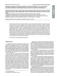
Nowadays, Single Pixel (SP) imaging has become an emerging paradigm for capturing high quality images using a single photo detector [1–4], in a low cost and high light throughput process with low memory requirement. These advantages have made SP imaging an excellent candidate for recording HyperSpectral (HS) volumes [5, 6], in particular, when it is combined with Fourier Transform Interferometry (FTI) [7, 8]. As schemed in Fig. 1 (dashed box on the right), FTI works on the principle of a Michelson interferometer. A coherent wide-band beam entering the FTI device is first divided into two beams by a Beam-Splitter (BS). Those beams are then reflected back either by a fixed mirror or by a moving mirror, controlling the Optical Path Difference (OPD) of the two beams, and interfere after being recombined by the BS. The resulting beam is later recorded by an external imaging sensor. Physical optics shows that the outgoing beam from the FTI, as a function of OPD ξ ∈ R, is the Fourier transform of the entering beam, as a function of wavenumber ν ∈ R. As an advantage, the spectral resolution of the HS volume can be increased by enlarging the range of recorded OPD values. However, in biomedical applications, this increase of resolution is limited by the tolerance of the biological elements against the light exposure. On the other hand, the theory of Compressed Sensing (CS) [9–11] has shown successful results [12–15] in reducing the amount of light exposure during the FTI acquisition, while the spectral resolution is preserved. We have proposed two compressive sensing-FTI methods in [16], i.e., Coded Illumination-FTI (CI-FTI) and Structured Illumination-FTI (SI-FTI), that can efficiently reduce the light exposure on the observed object. CI-FTI operates by temporal coding of the global light source, while in SI-FTI, spatial modulation of the illumination (e.g., by a spatial light modulator), allows for different OPD coding per spatial locations. Unlike the above-mentioned works, we here propose an FTI-based HS acquisition, that is constrained to use SP imaging. In the corresponding device, referred to as Single Pixel Fourier Transform Interferometry (SP-FTI), the light distribution is coded (or structured) in both OPD (or time) and spatial domains before being integrated into a single beam (unlike SI-FTI), using, e.g., collimating optics (see Sec. 3). While SPFTI has been implemented in food monitoring application [7], its theoretical analysis is not covered in the ∗ AM

is funded by the FRIA/FNRS. LJ is funded by the F.R.S.-FNRS.

1

Figure 1: Operating principles of SP-FTI. A continuous HS volume X c (e.g., observed from a confocal microscope) is spatially and temporally modulated from space-time coding of the light source.

literature. In this paper, adopting the stable and robust sampling strategies of Krahmer and Ward [17] for compressive imaging, we optimize SP-FTI sensing by following a Variable Density Sampling (VDS) of both the OPD domain and the Hadamard transformation of the spatial domain. This differs from a former work [8] where we considered multilevel sampling. In particular, our sampling strategy relies on the estimation of tight bounds on the local coherence between the 3D sensing and sparsity bases. The sensing basis is obtained from the Kronecker product of the Fourier (imposed by the FTI system) and Paley Hadamard (an aspect of our sensing design) bases and the sparsity basis is achieved by the Kronecker product of the 1D Haar wavelet and the 2D isotropic Haar wavelet bases. Our analysis in Appendix is versatile and could be extended to other SP imaging techniques. The rest of the paper is structured as follows. We first summarize the recovery guarantee associated with VDS theory in Sec. 2. After describing the principles of SP-FTI, our stable and robust compressive SP-FTI is proposed in Sec. 4. Numerical simulations are provided in Sec. 5. Notations: domain dimensions are represented by capital letters, e.g., K, M, N . Vectors, matrices, and data cubes are denoted by bold symbols. For any matrix (or vector) V ∈ CM ×N , V > and V ∗ represent the transposed and the conjugate transpose of V , respectively, and P V ⊗ W denotes the Kronecker product of two matrices V and W . The `p -norm of u reads kukp := ( i |ui |p )1/p , for p ≥ 1, with kuk := kuk2 . The identity matrix of dimension N is represented as I N . Finally, we use the asymptotic relations f . g (or f & g) if f ≤ c g (resp. g ≤ c f ) for two functions f and g and some value c > 0 independent of their parameters.

2

Compressed Sensing with random partial Orthonormal Bases

One interest of CS theory is to recover a signal x ∈ CN from a vector of noisy measurements [18] y = P Ω Φ∗ x + n,

(1)

where Ω = {ωj }M j=1 ⊂ JN K is a multiset of (non-unique) indices selected from a sampling strategy p, i.e., these indices are independently and identically distributed (i.i.d.) according to the probability mass function (pmf) p on JN K such that p(l) = P[ωj = l] for any l ∈ JN K and j ∈ JM K. The restriction operator is denoted by P Ω ∈ {0, 1}M ×N with (P Ω x)j = xωj and n models an additive noise. If x is assumed sparse (or well approximated by a sparse representation) in some basis Ψ, i.e., x = Ψs, with K := |supp (s)|  N , then the following proposition, which is a direct combination of [17, Thm. 5.2] and [16, Prop. 2.4], provides the conditions and guarantee under which x can be estimated from the noisy measurements y.

2

Proposition 1 (VDS guarantee). Let Φ, Ψ ∈ CN ×N be orthonormal sensing and sparsity bases, respectively. We assume a local coherence µl bounded as µl (Φ∗ Ψ) := maxj |(Φ∗ Ψ)l,j | ≤ κl , l ∈ JN K.

(2)

M & kκk2 K log(−1 ),

(3)

for some κl > 0, and κ := [κ1 , · · · , κN ]> . Suppose  ∈ (0, 1], K & log(N ),

and generate Ω = {ω1 , · · · , ωM } ⊂ JN K as explained above according to the pmf

p(l) := κ2l /kκk2 . (4) p Consider the diagonal matrix D ∈ RM ×M with djj = 1/ p(ωj ), j ∈ JM K. If x ∈ CN is a signal observed ˆ of the program by the noisy sensing model (1) with kDnk ≤ ε, then, the solution x ∆(y, p, Ω, Φ, Ψ) := arg minkΨ> uk1 s.t. kD(y − P Ω Φ∗ u)k ≤ ε,

(5)

u∈CNhs

ˆ k ≤ 2K −1/2 σK (Ψ> x) + ε, with probability exceeding 1 − , where σK (u) := ku − HK (u)k1 satisfies kx − x is the best K-term approximation error and HK is the hard thresholding operator that maps all but the K largest magnitude entries of the argument to zero.

3

From Nyquist to Compressive SP-FTI

Let us first study a Nyquist implementation of SP-FTI, i.e., collecting as many observations as the number of HS volume voxels, and where HS reconstruction can be achieved by a linear (inverse) transform. Let X ∈ RNν ×Np be the discretization of the HS volume X c (see Fig. 1) over Nν = Nξ wavenumber samples ¯p pixels in each x- and y-axis such that Np := N ¯ 2 . We assume that the light source provides constant and N p illumination during Nhs := Nξ Np time slots (associated to Nξ OPD samples). As shown in Fig. 1 (top-left), at each OPD sample lξ ∈ JNξ K, we consider a Coded Aperture (CA) that is programmed Np times with all p columns of the Hadamard basis Φhad ∈ {±1/ Np }Np ×Np (up to a rescaling, see Remark 1) [19]. Every programmed CA gives a spatially coded HS light beam, which is later integrated into a single beam, e.g., by means of an optical collimator. Following the principles of the FTI presented in Sec. 1, the light sensitive element records one Fourier coefficient (corresponding to the current OPD sample) of the spectral energy of the entering beam. Mathematically, the lth time slot corresponds to the lp th Hadamard pattern programmed at lξ th OPD point such that l = Np (lξ − 1) + lp ∈ JNhs K, lξ ∈ JNξ K, and lp ∈ JNp K. Therefore, each SP-FTI observation reads nyq ylnyq = P {lξ } Φ∗dft XΦhad P > = P {l} Φ∗sp x + nnyq , {lp } + nl l where x := vec(X), Φdft ∈ CNξ ×Nξ denotes the 1D discrete Discrete Fourier Transform (DFT) basis, Φsp := Φhad ⊗ Φdft and nnyq models a noise, which is assumed here to be an additive i.i.d. Gaussian noise, l nyq > 2 ] , the i.e., nnyq ∼i.i.d. N (0, σnyq ). By collecting all the observations in the vector y nyq := [y1nyq , · · · , yN l hs whole SP-FTI mixing model can be written as y nyq = Φ∗sp x + nnyq .

(6)

Remark p 1. As the Hadamard matrix contains ±Np −1/2 entries, it has to be properly transformed via Np ×Np Φbin := ( Np Φhad + 1Np 1> so that it can be implemented with 0’s and 1’s on a CA. Np )/2 ∈ {0, 1} However, the measurements (6) can be extracted from the actual measurements acquired by Φbin , as long as the all-on CA (associated with the first row of Hadamard matrix) is considered in the acquisition process [5, 6, 20]. We now propose a compressive form of SP-FTI, where only M Hadamard patterns (out of Nhs possible patterns) are programmed, i.e., we assume that CA blocks out the light illumination during the other Nhs −M time slots. The compressive SP-FTI system can be modeled as y sp = P Ω Φ∗sp x + n ∈ RM , 3

(7)

2 where n = [n1 , · · · , nM ]> with nl ∼i.i.d. N (0, σnyq ) and Ω = {ωj }M j=1 ⊂ JNhs K is the subsampled index set of Hadamard patterns. Considering Remark 1, a careful analysis reveals that the total light exposure received by the observed object during compressive SP-FTI acquisition is proportional to (M + Nξ )Np , compared to (Nhs + Nξ )Np in Nyquist SP-FTI, where the term Nξ is induced by Remark 1. The light exposure can thus be reduced by a factor of (M + Nξ )/(Nhs + Nξ ). In the next section, we optimize the pmf of each ωj according to a sparsity model of x, so that the number of required measurements M is minimized. This differs from [7] where a fixed number of Hadamard patterns, chosen uniformly at random, at every OPD point.

4

Main Results: Stable and Robust Compressive SP-FTI

W now provide a stable and robust scheme to recover every HS volume from our compressive SP-FTI system by following the general VDS scheme of Sec. 2, with special care to integrate the spatiospectral geometry of SP-FTI. As any other CS applications, HS data recovery from under-determined measurements in (7) requires an accurate low-complexity prior model on the HS volume. Our observations confirm that biological HS data commonly observed in FS share sparse/compressible representation in the Kronecker product of the 1-D Discrete Haar Wavelet (DHW) basis Ψdhw and the 2-D Isotropic Discrete Haar Wavelet (IDHW) basis Ψidhw . According to Prop. 1, given the noisy compressive SP-FTI measurements in (7), a stable and robust HS volume recovery can be achieved by solving ∆(y sp , p, Ω, Φsp , Ψsp ) in (5), where Ψsp := Ψidhw ⊗ Ψdhw denotes a 3-D analysis sparsity basis. We can now adjust the optimum pmf determining Ω from (4). Given κl ≥ µl (Φ∗sp Ψsp ), for l ∈ JNhs K, Prop. 1 shows that, for a fixed K and , we must record M & kκk2 K log(−1 ) SP-FTI measurements w.r.t. the pmf p(l) = κ2l /kκk2 with l ∈ JNhs K. We prove in Appendix that, in the context of SP-FTI, √ (8) κl := 2 min{1, 2−blog2 (max{lx ,ly }−1)c · |lξ − Nξ /2|−1/2 }, ¯p (ly −1)+lx , relates a 1D index l ∈ JNhs K and kκk2 . log(Nξ ) log(Np ), where l = l(lξ , lx , ly ) := Np (lξ −1)+ N ¯p K are the to a 3D index representation (lξ , lx , ly ) where lξ ∈ JNξ K denotes the OPD index and lx , ly ∈ JN spatial Hadamard “frequencies”. In this case, (4) in Prop. 1 reduces to p(l) = C min{1, |lξ − Nξ /2|−1 · | max{lx , ly }|−1 }, (9) P where C depends only on Nξ and Np and ensures that l p(l) = 1. Furthermore, under the requirements above, from Prop. 1 the estimation error achieved by the program ∆(y sp , p, Ω, Φsp , Ψsp ) is bounded by ˆ k ≤ 2K −1/2 σK (Ψ> kx − x sp x) + ε.

(10)

The following theorem summarizes this SP-FTI analysis. Theorem 1. Given  ∈ (0, 1] and K ∈ N such that K & log(Nhs ) and M & K log(Nξ ) log(Np ) log(−1 ).

(11)

Generate M random (non-unique) indices associated with an index set Ω = {ω1 , · · · , ωM } such that ωj ∼i.i.d. β for j ∈ JM K, with β a r.v. with the pmf in (9). Then, given the noisy compressive SP-FTI measurements y sp in (7), the HS volume x can be approximated by solving ∆(y sp , p, Ω, Φsp , Ψsp ) up to an error in (10) with probability exceeding 1 − . We observe that the optimum 1D pmf of selecting the rows of the matrix Φ∗sp is linked to the 3D geometry of the sensing domain. In (9), the probability of programming the CA decreases inversely proportional to the magnitude of the OPD point, i.e., its distance from the OPD origin. In addition, the probability of selecting a Hadamard pattern is inversely proportional to the maximum magnitude of spatial Hadamard “frequencies”. For the sake of comparison, a uniform density sampling strategy, i.e., p(l) = Nhs −1 for l ∈ JNhs K, and the sampling approach in [7] would require M & Nhs K log(−1 ) and M & Np K log(−1 ) measurements, respectively, which is equivalent to overexposing the observed object. 4

100 lν = 79

R-PE (R-phycoerythrin) Acridine orange TetraSpeck blue dye

lν = 96

Intensity

lν = 72

0 1

64

128

196

256

Wavenumber index (lν ) Figure 2: Three spatial maps of ground truth HS volume (left); the known spectral signatures of three fluorochromes (right).

30

SNR = 20 dB

CS rec.

SNR = 15 dB

25

SNR = 10 dB

RSNR (dB)

SNR = 5 dB

20

SNR = 0 dB

Fig. 4(a)

≈ 3.5 dB

15 10 5

ME rec. Fig. 4(b)

0

0.1 0.2 0.3 0.4 0.5 0.6 0.7 0.8 0.9

1

Measurement ratio (M/Nhs ) Figure 3: The performance of the proposed SP-FTI system.

5

Numerical results

We conduct several simulations to verify the performance of the proposed compressive SP-FTI on a simulated biological HS volume of size (Nξ , Np ) = (512, 642 ). We construct it by mixing the coefficients of three spectral bands of a synthetic biological RGB image selected from the benchmark images [21], with the known spectra of three common fluorochromes [22], see Fig. 2 (right). Compressive SP-FTI observations are formed according to (7), where the multiset Ω is randomly generated from the pmf (9) and the variance 2 is fixed w.r.t. to the desired Signal-to-Noise Ratio (SNR) reported in of the associated Gaussian noise σnyq 2 2 Nhs )). This sensing procedure is repeated over 10 random realizations Fig. 3, with SNR := 10 log(kxk /(σnyq of the noise and the multiset Ω. Fig. 3 depicts the average Reconstruction SNR (RSNR) in dB with ˆ k2 ). The value of ε is computed via the empirical 95th percentile curve of RSNR := 10 log(kxk2 /kx − x the weighted noise power kDnk over 100 Monte-Carlo realizations of the Gaussian noise and the index set Ω. We recover HS volumes through ∆(y sp , p, Ω, Φsp , Ψsp ) using SPGL1 toolbox [23], referred to as CS ˆ me := (P Ω Φ∗sp )† y sp , where † denotes the reconstruction, and the Minimal Energy (ME) problem, i.e., x pseudo-inverse operator [24]. Poor performance of the ME solution (see dashed lines) highlights the necessity of leveraging HS sparsity prior and VDS theory. Since ME reconstruction does not consider the noise power, its performance does not change w.r.t. different SNR values. On the contrary, the solution of ∆(y sp , p, Ω, Φsp , Ψsp ) is robust to the noisy measurements and is stable for compressible HS volumes. An example of the reconstructed HS volume w.r.t. M/Nξ ≈ (M + Nξ )/(Nhs + Nξ ) = 0.2 is visualized in Fig. 4. A comparison between these results and the ground truth values confirms that, even with 20% of the SP-FTI measurements, the spatial and spectral content of the HS volume is successfully preserved.

5

1 (c) spectrum at pixel (32,32)

RSNR = 18.70 dB

Normalized intensity

(a) CS rec., (32,32)

(b) ME rec.,

RSNR = 4.08 dB

Ground truth CS rec. ME rec.

0 1

64 128 196 Wavenumber index (lν )

256

Figure 4: Three spatial maps of the reconstructed HS volumes (left); the spectral content at the centered pixel (right).

6

Conclusion

We have proposed a compressive SP-FTI where the light source can be optimally structured (using Hadamard patterns) in order to minimize the light exposure imposed on the observed object and the number of measurements. Our method is practically plausible without any hardware modification to the initial SP-FTI [7]. The theoretical recovery guarantee of this work supports any application of SP-FTI. However, extending this work to a biologically friendly SP-FTI, where the total amount of light exposure is assumed fixed will be the scope of a future work. Tracing the effect of other sparsity bases on our local coherence analysis, e.g., the Daubechies wavelets [25], is also postponed to future investigations. APPENDIX: LOCAL COHERENCE BOUND We here provide a proof sketch for computing the bound on the local coherence µl (Φ∗sp Ψsp ) for l ∈ JNhs K ¯p (ly − 1) + lx between the 1D “l”and the 3D in (8). We recall the relation l = Np (lξ − 1) + lp , where lp = N ∗ ∗ “(lξ , lx , ly )” index representations. Noting that Φsp Ψsp = (Φhad Ψidhw ) ⊗ (Φ∗dft Ψdhw ), the definition of local coherence (2) gives (12) µl (Φ∗ Ψ) = µlξ (Φ∗dft Ψdhw ) · µlp (Φ∗had Ψidhw ). √ We have shown in [16, Prop. 5.3] that µlξ (Φ∗dft Ψdhw ) ≤ κξlξ := 2 min{1, |lξ − Nξ /2|−1/2 } and kκξ k2 . log(Nξ ). We prove in this work (see below) that µlp (Φ∗had Ψidhw ) = κplp := min{1, 2−blog2 (max{lx ,ly }−1)c }, ¯p ). Thus, replacing these values in (12) implies (8). Finally, we note kκk2 = and kκp k2 = 1 + 3 log2 (N ξ 2 p 2 kκ k · kκ k . ¯p = 2r , and Np = N ¯p2 , we first define 1-D Computation of µlp (Φ∗had Ψidhw ): For fixed integers r, N ` dyadic wavelet levels as T` := {l`−1 + 1, · · · , l` }, ` ∈ JrK with l` := 2 for ` ∈ JrK and T0 := {1}. In a matrix ¯ ¯ form, the 1D DHW basis in RNp ×Np can be constructed [25, 26] as      1 1 1 , I N¯p /2 ⊗ , Ψdhw := W N¯p = √ W N¯p /2 ⊗ 1 −1 2 with W 1 = [1]. Define also W 01 := [1] and Ψ0dhw

:=

W 0N¯p

     1 1 1 0 √ = W N¯p /2 ⊗ , I N¯p /2 ⊗ . 1 1 2

6

Up to a permutation of its columns, the 2D IDHW basis in RNp ×Np [25] can be constructed as Ψidhw = [Ψ0 , Ψ1 , Ψ2 , Ψ3 ], where Ψ0 := 1Np and > Ψ1:= [Ψ1,1 , · · · , Ψ1,r ], Ψ1,`:= (Ψ0dhw P > T` )⊗(Ψdhw P T` ), 0 > Ψ2:= [Ψ2,1 , · · · , Ψ2,r ], Ψ2,`:= (Ψdhw P > T` )⊗(Ψdhw P T` ), > Ψ3:= [Ψ3,1 , · · · , Ψ3,r ], Ψ3,`:= (Ψdhw P > T` )⊗(Ψdhw P T` ),

with ` ∈ JrK. The Np×Np Hadamard basis in Paley order [19, 27] is defined by Φhad :=H Np ∈ {±Np −1/2 }Np ×Np where      1 1 1 , H Np /2 ⊗ , H 1 := [1]. H Np := √ H Np /2 ⊗ 1 −1 2 Following these definitions, we can decompose the computation of local coherence as follows µlp (H ∗Np Ψidhw ) = max µlp (Aj,` ) =: κplp , j=1,2,3 `=1,··· ,r

(13)

where > ∗ A1,` := (H ∗N¯p W 0N¯p P > ¯p P T` ), ¯p W N T` ) ⊗ (H N > 0 ∗ A2,` := (H ∗N¯p W N¯p P > ¯p P T` ), ¯p W N T` ) ⊗ (H N > ∗ A3,` := (H ∗N¯p W N¯p P > ¯p P T` ). ¯p W N T` ) ⊗ (H N

Beside, we obtain by direct computation # H ∗N¯p /2 W N¯p /2 0N¯p /2×N¯p /2 , = H ∗N¯p /2 0N¯p /2×N¯p /2   ∗ H ∗N¯p /2 H N¯p /2 W 0N¯p /2 . = 0N¯p /2×N¯p /2 0N¯p /2×N¯p /2 "

H ∗N¯p W N¯p H ∗N¯p W 0N¯p We can show by recursion that

P Tt H ∗2r W 2r P > T` P Tt H ∗2r W 02r P > T`

(

if t = ` H ∗2t−1 , , 0|Tt |×|T` | , otherwise

(

H ∗2t−1 , if t = ` − 1 . 0|Tt |×|T` | , otherwise

=

=

−blog2 (j−1)c/2 This implies that µj (H ∗N¯p W N¯p P > }, if blog2 (j − 1)c = ` − 1 (and zero otherwise), T` ) = min{1, 2

( µj (H ∗N¯p W 0N¯p P > T` )

=

2−(`−1)/2 , if blog2 (j − 1)c ≤ ` − 2 . 0, otherwise

¯p (ly − 1) + lx ∈ JNp K, with lx , ly ∈ JN ¯p K, in order to decompose the We use again the relation lp = N computation of the local coherence of the matrices Aj,` , as follows ∗ 0 > µlp (A1,` ) = µlx (H ∗N¯p W N¯p P > ¯p W N ¯ p P T` ) T` ) · µly (H N ∗ > µlp (A2,` ) = µlx (H ∗N¯p W 0N¯p P > ¯ p P T` ) ¯p W N T` ) · µly (H N ∗ > µlp (A3,` ) = µlx (H ∗N¯p W N¯p P > ¯p P T` ). ¯p W N T` ) · µly (H N

By individual computation of µlp (Aj,` ) for j = 1, 2, 3, (13) gives µlp (Φ∗had Ψidhw ) = min{1, 2−blog2 (max{lx ,ly }−1)c } ¯p ), which completes the proof. and kκp k2 = 1 + 3 log2 (N 7

References [1] M. F. Duarte, M. A. Davenport, D. Takhar, J. N. Laska, T. Sun, K. E. Kelly, and R. G. Baraniuk, “Single-pixel imaging via compressive sampling,” IEEE signal processing magazine, vol. 25, no. 2, p. 83, 2008. [2] S. Sivankutty, V. Tsvirkun, O. Vanvincq, G. Bouwmans, E. R. Andresen, and H. Rigneault, “Nonlinear imaging through a fermats golden spiral multicore fiber,” Optics letters, vol. 43, no. 15, pp. 3638–3641, 2018. [3] S. Gu´erit, S. Sivankutty, C. Scott´e, J. A. Lee, H. Rigneault, and L. Jacques, “Compressive sampling approach for image acquisition with lensless endoscope,” arXiv preprint arXiv:1810.12286, 2018. [4] G. Davis, M. Maggioni, F. Warner, and F. Geshwind, “Hyperspectral analysis of normal and malignant colon tissue microarray sections using a novel DMD system,” in NIH Optical Imaging Workshop, 2004. [5] B. Roman, A. C. Hansen, and B. Adcock, “On asymptotic structure in compressed sensing,” arXiv preprint arXiv:1406.4178, 2014. [6] V. Studer, J. Bobin, M. Chahid, H. S. Mousavi, E. Cand`es, and M. Dahan, “Compressive fluorescence microscopy for biological and hyperspectral imaging,” Proceedings of the National Academy of Sciences, vol. 109, no. 26, pp. E1679–E1687, 2012. [7] S. Jin, W. Hui, Y. Wang, K. Huang, Q. Shi, C. Ying, D. Liu, Q. Ye, W. Zhou, and J. Tian, “Hyperspectral imaging using the single-pixel Fourier transform technique,” Scientific reports, vol. 7, p. 45209, 2017. [8] A. Moshtaghpour, J. M. Bioucas-Dias, and L. Jacques, “Compressive hyperspectral imaging: Fourier transform interferometry meets single pixel camera,” arXiv preprint arXiv:1809.00950, 2018. [9] D. L. Donoho, “Compressed sensing,” IEEE transactions on information theory, vol. 52, no. 4, pp. 1289–1306, 2006. [10] E. J. Cand`es and T. Tao, “Near-optimal signal recovery from random projections: Universal encoding strategies?” IEEE transactions on information theory, vol. 52, no. 12, pp. 5406–5425, 2006. [11] S. Foucart and H. Rauhut, A mathematical introduction to compressive sensing. 2013, vol. 1, no. 3.

Birkh¨auser Basel,

[12] A. Moshtaghpour, K. Degraux, V. Cambareri, A. Gonzalez, M. Roblin, L. Jacques, and P. Antoine, “Compressive hyperspectral imaging with Fourier transform interferometry,” in 3rd International Traveling Workshop on Interactions between Sparse models and Technology, 2016, pp. 27–29. [13] A. Moshtaghpour, V. Cambareri, L. Jacques, P. Antoine, and M. Roblin, “Compressive hyperspectral imaging using coded Fourier transform interferometry,” in Signal Processing with Adaptive Sparse Structured Representations workshop (SPARS), 2017. [14] A. Moshtaghpour and L. Jacques, “Multilevel illumination coding for Fourier transform interferometry in fluorescence spectroscopy,” arXiv preprint arXiv:1803.03217, 2018. [15] A. Moshtaghpour, V. Cambareri, K. Degraux, A. C. Gonzalez Gonzalez, M. Roblin, L. Jacques, and P. Antoine, “Coded-illumination Fourier transform interferometry,” in the Golden Jubilee Meeting of the Royal Belgian Society for Microscopy (RBSM), 2016, pp. 65–66. [16] A. Moshtaghpour, V. Cambareri, P. Antoine, M. Roblin, and L. Jacques, “A variable density sampling scheme for compressive Fourier transform interferometry,” 2018, arXiv:1801.10432v1. [17] F. Krahmer and R. Ward, “Stable and robust sampling strategies for compressive imaging,” IEEE transactions on image processing, vol. 23, no. 2, pp. 612–622, 2014.

8

[18] E. Cand`es and J. Romberg, “Sparsity and incoherence in compressive sampling,” Inverse problems, vol. 23, no. 3, pp. 969–985, 2007. [19] K. J. Horadam, Hadamard matrices and their applications.

Princeton university press, 2012.

[20] P. Sudhakar, L. Jacques, X. Dubois, P. Antoine, and L. Joannes, “Compressive imaging and characterization of sparse light deflection maps,” SIAM Journal on Imaging Sciences, vol. 8, no. 3, pp. 1824–1856, 2015. [21] P. Ruusuvuori, A. Lehmussola, J. Selinummi, T. Rajala, H. Huttunen, and O. Yli-Harja, “Benchmark set of synthetic images for validating cell image analysis algorithms,” in 16th European signal processing conference, 2008, pp. 1–5. [22] “Fluorophores.org - Database of fluorescent dyes, properties and applications,” retrieved on Jan. 5th, 2018. [Online]. Available: http://www.fluorophores.tugraz.at [23] E. Vandenberg and M. P. Friedlander, “Probing the pareto frontier for basis pursuit solutions,” SIAM Journal on Scientific Computing, vol. 31, no. 2, pp. 890–912, 2008. [24] E. J. Cand`es, J. Romberg, and T. Tao, “Robust uncertainty principles: Exact signal reconstruction from highly incomplete frequency information,” IEEE transactions on information theory, vol. 52, no. 2, pp. 489–509, 2006. [25] S. Mallat, A wavelet tour of signal processing: the sparse way.

Academic press, 2008.

[26] B. Fino, “Relations between Haar and Walsh/Hadamard transforms,” Proceedings of the IEEE, vol. 60, no. 5, pp. 647–648, 1972. [27] B. Falkowski and S. Rahardja, “Walsh-like functions and their relations,” IEE Proceedings-Vision, Image and Signal Processing, vol. 143, no. 5, pp. 279–284, 1996.

9