Abstract. Disjunctive Logic Programming (DLP) under the answer set seman- tics, often referred to as Answer Set Programming (ASP), is a powerful formalism.
Computable Functions in ASP: Theory and Implementation� Francesco Calimeri, Susanna Cozza, Giovambattista Ianni, and Nicola Leone Department of Mathematics, University of Calabria, I-87036 Rende (CS), Italy {calimeri,cozza,ianni,leone}@mat.unical.it
Abstract. Disjunctive Logic Programming (DLP) under the answer set semantics, often referred to as Answer Set Programming (ASP), is a powerful formalism for knowledge representation and reasoning (KRR). The latest years witness an increasing effort for embedding functions in the context of ASP. Nevertheless, at present no ASP system allows for a reasonably unrestricted use of function terms. Functions are either required not to be recursive or subject to severe syntactic limitations, if allowed at all in ASP systems. In this work we formally define the new class of finitely-ground programs, allowing for a powerful (possibly recursive) use of function terms in the full ASP language with disjunction and negation. We demonstrate that finitely-ground programs have nice computational properties: (i) both brave and cautious reasoning are decidable, and (ii) answer sets of finitely-ground programs are computable. Moreover, the language is highly expressive, as any computable function can be encoded by a finitely-ground program. Due to the high expressiveness, membership in the class of finitely-ground program is clearly not decidable (we prove that it is semi-decidable). We single out also a subset of finitely-ground programs, called finite-domain programs, which are effectively recognizable, while keeping computability of both reasoning and answer set computation. We implement all results in DLV, further extending the language in order to support list and set terms, along with a rich library of built-in functions for their manipulation. The resulting ASP system is very powerful: any computable function can be encoded in a rich and fully declarative KRR language, ensuring termination on every finitely-ground program. In addition, termination is “a priori” guaranteed if the user asks for the finite-domain check.
1 Introduction Disjunctive Logic Programming (DLP) under the answer set semantics, often referred to as Answer Set Programming (ASP) [1,2,3,4,5], evolved significantly during the last decade, and has been recognized as a convenient and powerful method for declarative knowledge representation and reasoning. Several systems supporting ASP have been implemented so far, thereby encouraging a number of applications in many real-world contexts ranging, e.g., from information integration, to frauds detection, to software �
Supported by M.I.U.R. within projects “Potenziamento e Applicazioni della Programmazione Logica Disgiuntiva” and “Sistemi basati sulla logica per la rappresentazione di conoscenza: estensioni e tecniche di ottimizzazione.”
M. Garcia de la Banda and E. Pontelli (Eds.): ICLP 2008, LNCS 5366, pp. 407–424, 2008. c Springer-Verlag Berlin Heidelberg 2008 �
408
F. Calimeri et al.
configuration, and many others. On the one hand, the above mentioned applications have confirmed the viability of the exploitation of ASP for advanced knowledge-based tasks. On the other hand, they have evidenced some limitations of ASP languages and systems, that should be overcome to make ASP better suited for real-world applications even in industry. One of the most noticeable limitations is the fact that complex terms like functions, sets and lists, are not adequately supported by current ASP languages/systems. Therefore, even by using state-of-the-art systems, one cannot directly reason about recursive data structures and infinite domains, such as XML/HTML documents, lists, time, etc. This is a strong limitation, both for standard knowledge-based tasks and for emerging applications, such as those manipulating XML documents. The strong need to extend DLP by functions is clearly perceived in the ASP community, and many relevant contributions have been recently done in this direction [6,7,8,9,10]. However, we still miss a proposal which is fully satisfactory from a linguistic viewpoint (high expressiveness) and suited to be incorporated in the existing ASP systems. Indeed, at present no ASP system allows for a reasonably unrestricted use of function terms. Functions are either required not to be recursive or subject to severe syntactic limitations, if allowed at all in ASP systems. This paper aims at overcoming the above mentioned limitations, toward a powerful enhancement of ASP systems by functions. The contribution is both theoretical and practical, and leads to the implementation of a powerful ASP system supporting (recursive) functions, sets, and lists, along with libraries for their manipulations. The main results can be summarized as follows: � We formally define the new class of finitely-ground (F G) DLP programs. This class allows for (possibly recursive) function symbols, disjunction and negation. We demonstrate that F G programs enjoy many relevant computational properties: • both brave and cautious reasoning are computable, even for non-ground queries; • answer sets are computable; • each computable function can be expressed by a F G program. � Since F G programs express any computable function, membership in this class is obviously not decidable (we prove that it is semi-decidable). For users/applications where termination needs to be “a priori” guaranteed, we define the class of finitedomain (F D) programs: • both reasoning and answer set generation are computable for F D programs (they are a subclass of F G programs), and, in addition, • recognizing whether a program is an F D program is decidable. � We extend the language with list and set terms, along with a rich library of built-in functions for lists and sets manipulations. � We implement all results and the full (extended) language in DLV, obtaining a very powerful system where the user can exploit the full expressiveness of F G programs (able to encode any computable function), or require the finite-domain check, getting the guarantee of termination. The system is available for downloading [11]; it is already in use in many universities and research centers throughout the world. For space limitations, we cannot include detailed proofs. Further documentation and examples are available on the web site [11].
Computable Functions in ASP: Theory and Implementation
409
2 DLP with Functions This section reports the formal specification of the DLP language with function symbols allowed. Syntax and notations. A term is either a simple term or a functional term. A simple term is either a constant or a variable. If t1 . . . tn are terms and f is a function symbol (functor) of arity n, then: f (t1 , . . . , tn ) is a functional term. Each ti , 1 ≤ i ≤ n, is a subterm of f (t1 , . . . , tn ). The subterm relation is reflexive and transitive, that is: (i) each term is also a subterm of itself; and (ii) if t1 is a subterm of t2 and t2 is subterm of t3 then t1 is also a subterm of t3 . Each predicate p has a fixed arity k ≥ 0; by p[i] we denote its i-th argument. If t1 , . . . , tk are terms, then p(t1 , . . . , tk ) is an atom. A literal l is of the form a or not a, where a is an atom; in the former case l is positive, and in the latter case negative. A rule r is of the form α1 ∨ · · · ∨ αk :- β1 , . . . , βn , not βn+1 , . . . , not βm . where m ≥ 0, k ≥ 0; α1 , . . . , αk and β1 , . . . , βm are atoms. We define H(r) = {α1 , . . . , αk } (the head of r) and B(r) = B + (r) ∪ B − (r) (the body of r), where B + (r) = {β1 , . . . , βn } (the positive body of r) and B − (r) = {not βn+1 , . . . , not βm } (the negative body of r). If H(r) = ∅ then r is a constraint; if B(r) = ∅ and |H(r)| = 1 then r is referred to as a fact. A rule is safe if each variable in that rule also appears in at least one positive literal in the body of that rule. For instance, the rule p(X, f (Y, Z)) :- q(Y ), not s(X). is not safe, because of both X and Z. From now on we assume that all rules are safe and there is no constraint.1 A DLP program is a finite set P of rules. As usual, a program (a rule, a literal) is said to be ground if it contains no variables. Given a program P , according with the database terminology, a predicate occurring only in facts is referred to as an EDB predicate, all others as IDB predicates. The set of all facts of P is denoted by Facts(P); the set of instances of all EDB predicates is denoted by EDB(P) (note that � EDB(P) ⊆ Facts(P)). The set of all head atoms in P is denoted by Heads(P ) = r∈P H(r). Semantics. The most widely accepted semantics for DLP programs is based on the notion of answer-set, proposed in [3] as a generalization of the concept of stable model [2]. Given a program P , the Herbrand universe of P , denoted by UP , consists of all (ground) terms that can be built combining constants and functors appearing in P . The Herbrand base of P , denoted by BP , is the set of all ground atoms obtainable from the atoms of P by replacing variables with elements from UP . A substitution for a rule r ∈ P is a mapping from the set of variables of r to the set UP of ground terms. A ground instance of a rule r is obtained applying a substitution to r. Given a program P the instantiation (grounding) grnd(P ) of P is defined as the set of all ground instances of its rules. Given a ground program P , an interpretation I for P is a subset of BP . A positive literal l = a (resp., a negative literal l = not a) is true w.r.t. I if a ∈ I (resp., a ∈ / I); it is false otherwise. Given a ground rule r, we say that r is satisfied w.r.t. 1
Under Answer Set semantics, a constraint :- B(r) can be simulated through the introduction of a standard rule fail :- B(r), not fail, where fail is a fresh predicate not occurring elsewhere in the program.
410
F. Calimeri et al.
G A (P )
G(P )
G C (P )
Fig. 1. Argument, Dependency and Component Graphs of the program in Example 1
I if some atom appearing in H(r) is true w.r.t. I or some literal appearing in B(r) is false w.r.t. I. Given a ground program P , we say that I is a model of P , iff all rules in grnd(P ) are satisfied w.r.t. I. A model M is minimal if there is no model N for P such that N ⊂ M . The Gelfond-Lifschitz reduct [3] of P , w.r.t. an interpretation I, is the positive ground program P I obtained from grnd(P ) by: (i) deleting all rules having a negative literal false w.r.t. I; (ii) deleting all negative literals from the remaining rules. I ⊆ BP is an answer set for a program P iff I is a minimal model for P I . The set of all answer sets for P is denoted by AS(P ). Dependency Graphs. We next define three graphs that point out dependencies among arguments, predicates, and components of a program. Definition 1. The Argument Graph G A (P ) of a program P is a directed graph containing a node for each argument p[i] of an IDB predicate p of P ; there is an edge (q[j], p[i]) iff there is a rule r ∈ P such that: (a) an atom p(t) appears in the head of r; (b) an atom q(v) appears in B + (r); (c) p(t) and q(v) share the same variable within the i-th and j-th term, respectively. Given a program P , an argument p[i] is said to be recursive with q[j] if there exists a cycle in G A (P ) involving both p[i] and q[j]. Roughly speaking, this graph keeps track of (body-head) dependencies between the arguments of predicates sharing some variable. It is actually a more detailed version of the commonly used (predicate) dependency graph, defined below. Definition 2. The Dependency Graph G(P ) of P is a directed graph whose nodes are the IDB predicates appearing in P . There is an edge (p2 , p1 ) in G(P ) iff there is some rule r with p2 appearing in B + (r) and p1 in H(r), respectively. The graph G(P ) suggests to split the set of all predicates of P into a number of sets (called components), one for each strongly connected component (SCC)2 of the graph itself. Given a predicate p, we denote its component by comp(p); with a small abuse of notation, we define also comp(l) and comp(a), where l is a literal and a is an atom, accordingly. In order to single out dependencies among components, a proper graph is defined next. 2
We recall here that a strongly connected component of a directed graph is a maximal subset S of the vertices, such that each vertex in S is reachable from all other vertices in S.
Computable Functions in ASP: Theory and Implementation
411
Definition 3. Given a program P and its Dependency Graph G(P ), the Component Graph of P , denoted G C (P ), is a directed labelled graph having a node for each strongly connected component of G(P ) and: (i) an edge (B, A), labelled “+”, if there is a rule r in P such that there is a predicate q ∈ A occurring in the head of r and a predicate p ∈ B occurring in the positive body of r; (ii) an edge (B, A), labelled “-”, if there is a rule r in P such that there is a predicate q ∈ A occurring in the head of r and a predicate p ∈ B occurring in the negative body of r, and there is no edge (B, A), with label “+”. Self-cycles are not considered. Example 1. Consider the following program P , where a is an EDB predicate: q(g(3)). p(X, Y ) :- q(g(X)), t(f (Y )).
s(X) ∨ t(f (X)) :- a(X), not q(X). q(X) :- s(X), p(Y, X).
Graphs G A (P ), G(P ) and G C (P ) are respectively depicted in Figure 1. There are three SCC in G(P ): C{s} = {s}, C{t} = {t} and C{p,q} = {p, q} which are the three nodes of G C (P ). An ordering among the rules, respecting dependencies pointed out by G C (P ), is defined next. Definition 4. A path in G C (P ) is strong if all its edges are labelled with “+”. If, on the contrary, there is at least an edge in the path labelled with “-”, the path is weak. A component ordering for a given program P is a total ordering �C1 , . . . , Cn � of all components of P s.t., for any Ci , Cj with i < j, both the following conditions hold: (i) there are no strong paths from Cj to Ci ; (ii) if there is a weak path from Cj to Ci , then there must be a weak path also from Ci to Cj .3 Example 2. Consider the graph G C (P ) of previous example. Both C{s} and C{t} are connected to C{p,q} through a strong path, while a weak path connects: C{s} to C{t} , C{t} to C{s} , C{p,q} to C{s} and C{p,q} to C{t} . Both γ1 = C{s} , C{t} , C{p,q} � and γ2 = C{t} , C{s} , C{p,q} � constitute component orderings for the program P . By means of the graphs defined above, it is possible to identify a set of subprograms (also called modules) of P , allowing for a modular bottom-up evaluation. We say that a rule r ∈ P defines a predicate p if p appears in H(r). Once a component ordering γ = C1 , . . . , Cn � is given, for each component Ci we define the module of Ci , denoted by P(Ci ), as the set of all rules r defining some predicate p ∈ Ci excepting those that define also some other predicate belonging to a lower component (i.e., certain Cj with j < i in γ). Example 3. Consider the program P of Example 1. If we consider the component ordering γ1 , the corresponding modules are: P (C{s} ) = { s(X) ∨ t(f (X)) :- a(X), not q(X). }, P (C{t}) = ∅, P (C{p,q} ) = {p(X, Y ) :- q(g(X)), t(f (Y ))., q(X) :- s(X), p(Y, X)., q(g(3)). }. 3
Note that, given the component ordering γ, Ci stands for the i-th component in γ, and Ci < Cj means that Ci precedes Cj in γ (i.e., i < j).
412
F. Calimeri et al.
The modules of P are defined, according to a component ordering γ, with the aim of properly instantiating all rules. It is worth remembering that we deal only with safe rules, i.e., all variables appear in the positive body; it is therefore enough to instantiate the positive body. Furthermore, any component ordering γ guarantees that, when r ∈ P (Ci ) is instantiated, each nonrecursive predicate p appearing in B + (r) is defined in a lower component (i.e., in some Cj with j < i in γ). It is also worth remembering that, according to how the modules of P are defined, if r is a disjunctive rule, then it is associated only to a unique module P (Ci ), chosen in such a way that, among all components Cj such that comp(a) = Cj for some a ∈ H(r), it always holds i ≤ j in γ (that is, the disjunctive rule is associated only to the (unique) module corresponding to the lowest component among those “covering” all predicates featuring some instance in the head of r). This implies that the set of the modules of P constitute an exact partition for it.
3 Finitely-Ground Programs In this section we introduce a subclass of DLP programs, namely finitely-ground (F G) programs, having some nice computational properties. Since the set of ground instances of a rule might be infinite (because of the presence of function symbols), it is crucial to try to identify those that really matter in order to compute answer sets. Supposing that S contains all atoms that are potentially true, next definition singles out the relevant instances of a rule. Definition 5. Given a rule r and a set S of ground atoms, an S-restricted instance of r is a ground instance r� of r such that B + (r� ) ⊆ S. The set of all S-restricted instances of a program P is denoted as InstP (S). Note that, for any S ⊆ BP , InstP (S) ⊆ grnd(P ). Intuitively, this helps selecting, among all ground instances, those somehow supported by a given set S. Example 4. Consider the following program P : t(f (1)).
t(f (f (1))).
p(1).
p(f (X)) :- p(X), t(f (X))).
The set InstP (S) of all S-restricted instances of P , w.r.t. S = F acts(P ) is: t(f (1)).
t(f (f (1))).
p(1).
p(f (1)) :- p(1), t(f (1)).
The presence of negation allows for identifying some further rules which do not matter for the computation of answer sets, and for simplifying the bodies of some others. This can be properly done by exploiting a modular evaluation of the program that relies on a component ordering. Definition 6. Given a program P , a component ordering C1 , . . . , Cn �, a set Si of ground rules for Ci , and a set of ground rules R for the components preceding Ci , the simplification Simpl(Si , R) of Si w.r.t. R is obtained from Si by: 1. deleting each rule whose body contains some negative body literal not a s.t. a ∈ F acts(R), or whose head contains some atom a ∈ F acts(R);
Computable Functions in ASP: Theory and Implementation
413
2. eliminating from the remaining rules each literal l s.t.: – l = a is a positive body literal and a ∈ F acts(R), or – l = not a is a negative body literal, comp(a) = Cj with j < i, and a ∈ / Heads(R). Assuming that R contains all instances of the modules preceding Ci , Simpl(Si , R) deletes from Si all rules whose body is certainly false or whose head is certainly already true w.r.t. R, and simplifies the remaining rules by removing from the bodies all literals that are true w.r.t. R. Example 5. Consider the following program P : t(1). s(1). q(X) :- t(X).
s(2). p(X) :- s(X), not q(X).
It is easy to see that C1 = {q}, C2 = {p}� is the only component ordering for P . If we consider R = EDB(P ) = { t(1)., s(1)., s(2). } and S1 = {q(1) :- t(1).}, then Simpl(S1 , R) = {q(1).} (i.e., t(1) is eliminated from body). Considering then R = {t(1)., s(1)., s(2)., q(1).} and S2 = { p(1) :- s(1), not q(1)., p(2) :- s(2), not q(2). }, after the simplification we have Simpl(S2, R) = {p(2).}. Indeed, s(2) is eliminated as it belongs to F acts(R) and not q(2) is eliminated because comp(q(2)) = / Heads(R); in addition, C1 precedes C2 in the component ordering and the atom q(2) ∈ rule p(1) :- s(1), not q(1). is deleted, since q(1) ∈ F acts(R). We are now ready to define an operator Φ that acts on a module of a program P in order to: (i) select only those ground rules whose positive body is contained in a set of ground atoms consisting of the heads of a given set of rules; (ii) perform a further simplification among these rules by means of the Simpl operator. Definition 7. Given a program P , a component ordering C1 , . . . , Cn �, a component Ci , the module M = P (Ci ), a set X of ground rules of M , and a set R of ground rules belonging only to EDB(P) or to modules of components Cj with j < i, let ΦM,R (X) be the transformation defined as follows: ΦM,R (X) = Simpl(InstM (Heads(R ∪ X)), R). Example 6. Let P be the program of Example 1 where the extension of EDB predicate a is {a(1)}. Considering the component C1 = {s}, the module M = P (C1 ), and the sets X = ∅ and R = {a(1)}, we have:
ΦM,R (X) = Simpl(InstM (Heads(R ∪ X)), R) = = Simpl(InstM ({a(1)}), {a(1).}) = = Simpl({s(1) ∨ t(f (1)) :- a(1), not q(1).}, {a(1).}) = = {s(1) ∨ t(f (1)) :- not q(1).}.
The operator defined above has the following important property. Proposition 1. ΦM,R always admits a least fixpoint Φ∞ M,R (∅). Proof. (Sketch) The statement follows from Tarski’s theorem [12]), noting that ΦM,R is a monotonic operator and that a set of rules forms a meet semilattice under set containment. �
414
F. Calimeri et al.
By properly composing consecutive applications of Φ∞ to a component ordering, we can obtain an instantiation which drops many useless rules w.r.t. answer sets computation. Definition 8. Given a program P and a component ordering γ = C1 , . . . , Cn � for P , the intelligent instantiation P γ of P for γ is the last element Sn of the sequence s.t. S0 = EDB(P ), Si = Si−1 ∪ Φ∞ Mi ,Si−1 (∅), where Mi is the program module P (Ci ). Example 7. Let P be the program of Example 1 where the extension of EDB predicate a is {a(1)}; considering the component ordering γ = C1 = {s}, C2 = {t}, C3 = {p, q}� we have: – – – –
S0 S1 S2 S3
= {a(1).}; = S0 ∪ Φ∞ M1 ,S0 (∅) = {a(1)., s(1) ∨ t(f (1)) :- not q(1).}; = S1 ∪ Φ∞ M2 ,S1 (∅) = {a(1)., s(1) ∨ t(f (1)) :- not q(1).}; = S2 ∪ Φ∞ M3 ,S2 (∅) = {a(1)., s(1) ∨ t(f (1)) :- not q(1)., q(g(3))., p(3, 1) :- q(g(3)), t(f (1))., q(1) :- s(1), p(3, 1).}.
Thus, the resulting intelligent instantiation P γ of P for γ is: a(1). q(g(3)). p(3, 1) :- q(g(3)), t(f (1)).
s(1) ∨ t(f (1)) :- not q(1). q(1) :- s(1), p(3, 1).
We are now ready to define the class of F G programs. Definition 9. A program P is finitely-ground (F G) if P γ is finite, for every component ordering γ for P . Example 8. The program of Example 1 is F G: P γ is finite both when γ =
C{s} , C{t} , C{p,q} � and when γ = C{t} , C{s} , C{p,q} � (i.e., for the both of two component orderings for P ).
4 Properties of Finitely-Ground Programs In this section the class of F G programs is characterized by identifying some key properties. The next theorem shows that we can compute the answer sets of an F G program by considering intelligent instantiations, instead of the theoretical (possibly infinite) ground program. Theorem 1. Let P be an F G program and P γ be the intelligent instantiation of P w.r.t. a component ordering γ for P . Then, AS(P ) = AS(P γ ) (i.e., P and P γ have the same answer sets). Proof. (Sketch) Given γ = C1 , . . . , Cn �, let denote, as usual, by Mi the program module �nP (Ci ), and consider the sets S0 , . . . , Sn as defined in Definition 8. Since P = i=0 Mi the theorem can be proven by showing that: AS(Sk ) = AS(
�k i=0
Mi ) for 1 ≤ k ≤ n
Computable Functions in ASP: Theory and Implementation
415
where M0 denotes EDB(P ). The equation clearly holds for k = 0. Assuming that it holds for all k ≤ j, we can show that it holds for k = j + 1. The equation above can be rewritten as: AS(Sk−1 ∪ Φ∞ Mk ,Sk−1 (∅)) = AS(
�k−1 i=0
Mi ∪ Mk ) ) for 1 ≤ k ≤ n
The induction hypothesis allows us to assume that the equivalence AS(Sk−1 ) = � AS( k−1 i=0 Mi ) holds. A careful analysis is needed of the impact that the addition of � k−1 Mk to i=0 Mi has on answer sets of Sk ; in order to prove the theorem, it is enough to show that the set Φ∞ Mk ,Sk−1 (∅) does not drop any “meaningful” rule w.r.t. Mk . If we disregard the application of the Simpl operator, i.e. we consider the operator Φ performing only InstMk (Heads(Sk−1 ∪ ∅)), then Φ∞ Mk ,Sk−1 (∅) clearly generates all rules having a chance to have a true body in any answer set; omitted rules have a false body in every answer set, and are therefore irrelevant. The application of Simpl does not change the scenario: it relies only on previously derived facts, and on the absence of atoms from heads of previously derived ground rules.4 If a fact q has been derived in a previous component, then any rule featuring q in the head or not q in the body is deleted, as it is already satisfied and cannot contribute to any answer set. The simplification operator also drops, from the bodies, positive atoms of lower components appearing as facts, as well as negative atoms belonging to lower components which do not appear in the head of any already generated ground rule. The presence of facts in the bodies is obviously irrelevant, and the deleted negative atoms are irrelevant as well. Indeed, by construction of the component dependency graph, while instantiating a module, all rules defining atoms of lower components have been already instantiated. Thus, atoms of lower components not appearing in the head of any generated rule, have no chances to be true in any answer set. � Corollary 1. An F G program has finitely many answer sets, and each of them is finite. Theorem 2. Given an F G program P , AS(P ) is computable. Proof. Note that by Theorem 1, answer sets of P can be obtained by computing the answer sets of P γ for a component ordering γ of choice, which can be easily computed. Then, P γ can be obtained by computing the sequence of fixpoints of Φ specified in Definition 8. Each fixpoint is guaranteed to be finitely computable, since the program is finitely-ground. � From this property, the main result below immediately follows. Theorem 3. Cautious and brave reasoning over F G programs are computable. Computability holds even for non-ground queries. As the next theorem shows, the class of F G programs allows for the encoding of any computable function. 4
Note that, due to the elimination of true literals performed by the simplification operator Simpl, the intelligent instantiation of a rule with a non empty body may generate some facts.
416
F. Calimeri et al.
Theorem 4. Given a recursive function f , there exists a DLP program Pf such that, for any input x for f , Pf ∪ θ(x) is finitely-ground and AS(Pf ∪ θ(x)) encodes f (x), for θ a simple function encoding x by a set of facts. Proof. (Sketch) We can build a positive program Pf , which encodes the Turing machine Mf corresponding to f (see [11]). For any input x to Mf , (Pf ∪ θ(x))γ is finite for any component ordering γ, and AS(Pf ∪ θ(x)) contains an appropriate encoding of f (x). � Note that recognizing F G programs is semi-decidable, yet not decidable: Theorem 5. Recognizing whether P is an F G program is R.E.-complete. Proof. (Sketch) Semi-decidability is shown by implementing an algorithm evaluating the sequence given in Definition 8, and answering “yes” if the sequence converges in finite time. On the other hand, given a Turing machine M and an input tape x, it is possible to write a corresponding program PM and a set θ(x) of facts encoding x, such that M halts on input x iff PM ∪ θ(x) is finitely-ground. The program PM is the same as in the proof of Theorem 4 and reported in [11]. �
5 Finite-Domain Programs In this section we single out a subclass of F G programs, called finite-domain (F D) programs, which ensures the decidability of recognizing membership in the class. Definition 10. Given a program P , the set of finite-domain arguments (F D arguments) of P is the maximal (w.r.t. inclusion) set FD(P ) of arguments of P such that, for each argument q[k] ∈ FD(P ), every rule r with head predicate q satisfies the following condition. Let t be the term corresponding to argument q[k] in the head of r. Then, 1. either t is variable-free, or 2. t is a subterm 5 of (the term of) some F D argument of a positive body predicate, or 3. every variable appearing in t also appears in (the term of) a F D argument of a positive body predicate which is not recursive with q[k]. If all arguments of the predicates of P are F D, then P is said to be an F D program. Intuitively, F D arguments can range only on a finite set of different ground values. Observe that FD(P ) is well-defined; indeed, it is easy to see that there always exists, and it is unique, a maximal set satisfying Definition 10 (trivially, given two sets A1 and A2 of F D arguments for a program P , the set A1 ∪ A2 is also a set of F D arguments for P ). Example 9. The following is an example of F D program: q(f (0)). 5
q(X) :- q(f (X)).
The condition can be made less strict considering other notions, as, e.g., the norm of a term [13,14,15].
Computable Functions in ASP: Theory and Implementation
417
Indeed q[1] is the only argument in the program and it is an F D argument, since the two occurrences of q[1] in a rule head satisfy first and second condition of Definition 10, respectively. Example 10. The following is not an F D program: q(f (0)). s(f (X)) :- s(X).
q(X) :- q(f (X)). v(X) :- q(X), s(X).
We have that all arguments belong to FD(P ), except for s[1]. Indeed, s[1] appears as head argument in the third rule with term f (X), and: (i) f (X) is not variable-free; (ii) f (X) is not a subterm of some term appearing in a positive body F D argument; (iii) there is no positive body predicate which is not recursive with s and contains X. By the following theorems we now point out two key properties of F D programs. Theorem 6. Recognizing whether P is an F D program is decidable. Proof. (Sketch) An algorithm deciding whether P is F D or not can be defined as follows. Arguments of predicates in P are all supposed to be F D at first. If at least one rule is found, such that for an argument of an head predicate none of the three conditions of Definition 10 holds, then P is recognized as not being an F D program. If no such rule is found, the answer is positive. � Theorem 7. Every F D program is an F G program. Proof. (Sketch) Given an F D program P , it is possible to find a priori an upper bound for the maximum nesting level6 of the terms appearing in P γ , for any component ordering γ for P . This is given by max nl = (n + 1) ∗ m, where m is the maximum nesting level of the terms in P , and n is the number of components in γ. Indeed, given that P is an F D program, it is easy to see that the maximum nesting level cannot increase because of recursive rules, since, in this case, the second condition of Definition 10 forces a sub-term relationships between head and body predicates. Hence, the maximum nesting level can increase only because of body-head dependencies among predicates of different components. We can now compute the set of all possible ground terms t obtained by combining all constants and function symbols appearing in P , such that the nesting level of t is less or equal to max nl. This is a finite set, and clearly a superset of the ground terms appearing in P γ . Thus, P γ is necessarily finite. � The results above allow us to state the following properties for F D programs. Corollary 2. Let P be an F D program, then: 1. P has finitely many answer sets, and each of them is finite. 2. AS(P ) is computable; 3. skeptical and credulous reasoning over P are computable. Computability holds even if the query at hand is not ground. 6
The nesting level of a ground term is defined inductively as follows: (i) a constant term has nesting level zero; (ii) a functional term f (t1 , . . . , tn ) has nesting level equal to the maximum nesting level among t1 , . . . , tn plus one.
418
F. Calimeri et al.
6 An ASP System with Functions, Sets, and Lists In this section we briefly illustrate the implementation of an ASP system supporting the language herein presented. Such system actually features an even richer language, that, besides functions, explicitly supports also complex terms such as lists and sets, and provides a large library of built-in predicates for facilitating their manipulation. Thanks to such extensions, the resulting language becomes even more suitable for easy and compact knowledge representation tasks. Language. We next informally point out the peculiar features of the fully extended language, with the help of some sample programs. In addition to simple and functional terms, there might be also list and set terms; a term which is not simple is said to be complex. A list term can be of two different forms: (i) [t1 , . . . , tn ], where t1 , . . . , tn are terms; (ii) [h|t], where h (the head of the list) is a term, and t (the tail of the list) is a list term. Examples for list terms are: [jan, f eb, mar, apr, may, jun], [jan | [f eb, mar, apr, may, jun]], [[jan, 31] | [[f eb, 28], [mar, 31], [apr, 30], [may, 31], [jun, 30]]]. Set terms are used to model collections of data having the usual properties associated with the mathematical notion of set. They satisfy idempotence (i.e., sets have no duplicate elements) and commutativity (i.e., two collections having the same elements but with a different order represent the same set) properties. A set term is of the form: {t1 , . . . , tn }, where t1 , . . . , tn are ground terms. Examples for set terms are: {red, green, blue}, {[red, 5], [blue, 3], [green, 4]}, {{red, green}, {red, blue}, {green, blue}}. Note that duplicated elements are ignored, thus the sets: {red, green, blue} and {green, red, blue, green} are actually considered as the same. As already mentioned, in order to easily handle list and set terms, a rich set of builtin functions and predicates is provided. Functional terms prefixed by a # symbol are built-in functions. Such kind of functional terms are supposed to be substituted by the values resulting from the application of a functor to its arguments, according to some predefined semantics. For this reason, built-in functions are also referred to as interpreted functions. Atoms prefixed by # are, instead, instances of built-in predicates. Such kind of atoms are evaluated as true or false by means of operations performed on their arguments, according to some predefined semantics7 . Some simple built-in predicates are also available, such as the comparative predicates equality, less-than, and greater-than (=, ) and arithmetic predicates like successor, addition or multiplication, whose meaning is straightforward. A pair of simple examples about complex terms and proper manipulation functions follows. Another interesting example, i.e., the Hanoi Tower problem, is reported in [11]. Example 11. Given a directed graph, a simple path is a sequence of nodes, each one appearing exactly once, such that from each one (but the last) there is an edge to the next in the sequence. The following program derives all simple paths for a directed graph, starting from a given edge relation: path([X, Y ]) :- edge(X, Y ). path([X|[Y |W ]]) :- edge(X, Y ), path([Y |W ]), not #member(X, [Y |W ]). 7
The specification of the entire library for lists and sets manipulation is available at [11].
Computable Functions in ASP: Theory and Implementation
419
The first rule builds a simple path as a list of two nodes directly connected by an edge. The second rule constructs a new path adding an element to the list representing an existing path. The new element will be added only if there is an edge connecting it to the head of an already existing path. The external predicate #member (which is part of the above mentioned library for lists and sets manipulation) allows to avoid the insertion of an element that is already included in the list; without this check, the construction would never terminate in the presence of circular paths. Even if not an F D program, it is easy to see that this is an F G program; thus, the system is able to effectively compute the (in this case, unique) answer set. Example 12. Let us imagine that the administrator of a social network wants to increase the connections between users. In order to do that, (s)he decides to propose a connection to pairs of users that result, from their personal profile, to share more than two interests. If the data about users are given by means of EDB atoms of the form user(id, {interest1 , . . . , interestn }), the following rule would compute the set of common interests between all pairs of users: sharedInterests(U1, U2 , #intersection(S1 , S2 )) :- user(U1 , S1 ), user(U2 , S2 ), U1 �= U2 .
where the interpreted function #intersection takes as input two sets and returns their intersection. Then, the predicate selecting all pairs of users sharing more than two interests could be defined as follows: proposeConnection(pair(U1 , U2 )) :- sharedInterests(U1, U2 , S), #card(S) > 2.
Here, the interpreted function #card returns the cardinality of a given set, which is compared to the constant 2 by means of the built-in predicate “>”. Implementation. The presented language has been implemented on top of the stateof-the-art ASP system DLV [16]. Complex terms have been implemented by using a couple of built-in predicates for packing and unpacking them (see below). These functions, along with the library for lists and sets manipulation have been incorporated in DLV by exploiting the framework introduced in [17]. In particular, support for complex terms is actually achieved by suitably rewriting the rules they appear in. The resulting rewritten program does not contain complex terms any more, but a number of instances of proper built-in predicates. We briefly illustrate in the following how the rewriting is performed in case of functional terms; the cases of list and set terms are treated analogously. Firstly, any functional term t = f (X1 , . . . , Xn ), appearing in some rule r ∈ P , is replaced by a fresh variable F t and then, one of the following atom is added to B(r): - #f unction pack(F t, f, X1 , . . . , Xn ) if t appears in H(r); - #f unction unpack(F t, f, X1 , . . . , Xn ) if t appears in B(r). This transformation is applied to the rule r until no functional terms appear in it. The role of an atom #f unction pack is to build a functional term starting from a functor and its arguments; while an atom #f unction unpack acts unfolding a functional term to give values to its arguments. So, the former binds the F t variable, provided that all
420
F. Calimeri et al.
other terms are already bound, the latter binds (checks values, in case they are already bound) the X1 , . . . , Xn variables according to the binding for the F t variable (the whole functional term). Example 13. The rule: p(f (f (X))) :- q(X, g(X, Y )). will be rewritten as follow: p(F t1 ) :- #f unction pack(F t1 , f, F t2 ), #f unction pack(F t2 , f, X), q(X, F t3 ), #f unction unpack(F t3 , g, X, Y ).
Note that rewriting the nested functional term f (f (X)) requires two #f unction pack atoms in the body: (i) for the inner f function having X as argument and (ii) for the outer f function having as argument the fresh variable F t2 , representing the inner functional term. The resulting ASP system is indeed very powerful: the user can exploit the full expressiveness of F G programs (plus the ease given by the availability of complex terms), at the price of giving the guarantee of termination up. In this respect, it is worth stating that the system grounder fully complies with the definition of intelligent instantiation introduced in this work (see Section 3 and Definition 8). This implies, among other things, that the system is guaranteed to terminate and correctly compute all answer sets for any program resulting as finitely-ground. Nevertheless, the system features a syntactic F D programs recognizer, based on the algorithm sketched in Theorem 6. This kind of finite-domain check, which is active by default, ensures a priori computability for all accepted programs. The system prototype, called DLV-complex, is available at [11]; the above mentioned library for list and set terms manipulation is available for free download as well, together with a reference guide and a number of examples. Some preliminary tests have been carried out in order to measure how much the new features cost in terms of performances: rewriting times are negligible; the cost of evaluating function terms (pack/unpack functions) is low (about 1.5 times a comparison built-in as ’