P1: GCR pp655-jons-454093
JONS.cls
November 15, 2002
16:37
C 2002) Journal of Network and Systems Management, Vol. 10, No. 4, December 2002 (°
Optimizing Management Functions in Distributed Systems Hasina Abdu,1,3 Hanan Lutfiyya,2 and Michael A. Bauer2
With the increased availability and complexity of distributed systems comes a greater need for solutions to assist in the management of distributed systems. Despite the significant contributions made towards the development of management tools that monitor and control distributed systems, little has been done to address issues such as optimizing the execution of management functions with respect to system and management requirements. This paper presents a management optimization model in which management agents and managed objects are efficiently configured on the basis of a set of system and management requirements. We illustrate our model and describe its implementation through a Branch- and Bound-based algorithm and a web-based interface. The latter enables users to specify the requirements used by the optimization algorithm to determine efficient management configurations. It also includes an XML-based interface through which management agents can be started independent of the underlying platforms. Performance characteristics of the proposed algorithm as well as experimental results to illustrate the validity of the model are also described. KEY WORDS: Distributed systems management; management agents; management configuration; management policies; optimization.
1. INTRODUCTION The primary goal of distributed systems management is to ensure efficient use of resources and provide timely service to users. Management has evolved from simple centralized static solutions to dynamic web-based solutions involving heterogeneous computing systems. Playing a central role in such systems are entities referred to as management agents. Management agents carry out management 1 Department
of Computer and Information Sciences, University of Michigan—Dearborn, Dearborn, Michigan. 2 Department of Computer Science, University of Western Ontario, Ontario, Canada. 3 To whom correspondence should be addressed at 4901 Evergreen Rd., Room 122A ELB, College of Engineering and Computer Science, University of Michigan—Dearborn, Dearborn, Michigan 48128. E-mail:
[email protected] 505 C 2002 Plenum Publishing Corporation 1064-7570/02/1200-0505/0 °
P1: GCR pp655-jons-454093
506
JONS.cls
November 15, 2002
16:37
Abdu, Lutfiyya, and Bauer
activities by interacting with managed objects, i.e., abstractions of the managed components in a distributed system,4 to monitor their behavior and perform control actions on them. Agents may vary from a collection of management interface routines used to instrument managed applications, to active, independent processes such as SNMP [1] or CMIP [2] agents. Some agents may possess the capabilities of both monitoring and controlling functions. Other agents may also possess some analysis capabilities, which allow them to analyze and determine any needed control actions. Agents also vary in their implementation and the platforms they execute. For example, with the advent of mobile agent platforms, agents can also be transported across the network instead of transferring the data itself (e.g., [3]). Web-based management (e.g., [4]), management environment under CORBA (e.g., [5]), and message-oriented middleware are other examples of possible frameworks. We do not assume any specific implementation or agent framework, thus focusing on a generic solution. 1.1. Management Policies and Management Configurations We use the term management policy5 to refer to the specification of one or more operations on a set of attributes of one or more managed objects. A management policy will, therefore, determine what agents are needed for management, based on the data it specifies. In addition, it specifies where agents should collect the data from and what operation to execute on such data. For example, if a management policy specifies the monitoring of the packets transmitted by a given host in the system, the agent(s) deployed for management must be “equipped” to collect such data. In addition, if policies specify a specific analysis operation (e.g., standard deviation), only agents that can execute such operations can be deployed. For each management policy there will be different ways in which agents can be instantiated, as well as different ways in which agents can communicate with each other and with managed objects. We use the term management configurations to refer to the different “arrangements” of management agents and managed objects that correspond to a given set of management policies. For example, consider a management policy that requires the average of the CPU loads of four hosts. Figure 1 illustrates different management configurations. Managed objects are in different hosts and are represented by circles and the cubes represent management agents. The arrows illustrate the flow of information between the different agents and between managed objects and management agents. In Fig. 1(a), a single agent 4 In
this paper, we adopt an interchangeable use of the term managed objects to refer to both the abstractions of managed components as well as the actual managed components. 5 Our definition of policy differs from the traditional definitions found in Ref. [6, 7]. We focus on the information representing the attributes of managed objects and the analysis operations to be executed on a set of monitored data.
P1: GCR pp655-jons-454093
JONS.cls
November 15, 2002
16:37
Optimizing Management Functions in Distributed Systems
507
Fig. 1. Different configurations for a sample management policy.
collects the CPU load from each host and determines the average CPU load. In Fig. 1(b), the collection and analysis are done by separate agents. An agent extracts the CPU load from a host and sends the CPU information to an agent that performs the average computation. In Fig. 1(c), agents are arranged such that partial average values are obtained in parallel. In Fig. 1(d) agents are arranged such that partial sums are obtained in parallel and the average is obtained by a single agent. Unlike Fig. 1(c), where an agent either collects or analyzes data, in Fig. 1(d) agents collect and analyze data. It is not obvious which management configuration to use. For example, in the management configuration in Fig. 1(a), the time to determine the average CPU load is high if the number of managed objects is high. The single agent is a bottleneck. The management configurations represented in Figs. 1(b)–(d) illustrate different amounts of parallelism that can be used to reduce the amount of time to determine the average CPU load. Increased parallelism usually means more resource consumption. For example, it is obvious that the management configuration in Fig. 1(b) uses more CPU cycles than does the management configuration in Fig. 1(a). In addition, if all the agents are started on different hosts in the system, more network bandwidth is needed. The management configuration in Fig. 1(c) uses more CPU cycles and generates more network traffic (depending on the location of agents) than do the configurations in Figs. 1(a) and (b), but it may deliver a faster response for a larger number of managed objects. The configurations in Fig. 1 differ in resource usage and the time to collect and analyze the data. There is a trade-off in the consumption of system resources, i.e.,
P1: GCR pp655-jons-454093
JONS.cls
November 15, 2002
508
16:37
Abdu, Lutfiyya, and Bauer
some configurations consume fewer resources, but may result in slower execution of management functions. The choice of a management configuration partially depends on the priorities of the managers. It should be noted that this example is very simplistic and is used for illustration purposes. Additional complexity and diversity is to be expected from the mapping of a more realistic set of management policies to a set of management configurations. 1.2. Problem Statement As illustrated earlier, there is a trade-off between resource consumption by agents and managed objects (referred to as management overhead) and the time it takes for a result to be returned. Ideally, we would like to minimize resource consumption. In Section 1.1, this would mean choosing the management configuration in Fig. 1(a). However, this may be too slow. If we minimize response time without considering the management overhead, then the management configuration in Fig. 1(c) may be a better choice. On the other hand, this may be unacceptable in that it may generate too much network traffic or consume too many CPU cycles. We have yet to consider the trade-off between the consumption of the different resources in the system. For example, in Fig. 1, having an agent on each of the hosts from which the CPU load is to be collected reduces network traffic, but the memory usage and CPU load on that host increases. A consideration in choosing a management configuration is based on which resource usage is to be minimized. In addition to requirements on resource usage, managers may impose other restrictions that must be satisfied by management configurations. For example, it may be that no agent must be started on the same host as the web server or that an agent must not be started unless it collects data from at least three managed objects. Because of the dynamic nature of distributed systems, the management requirements, the requirements defined on resource usage, and the specified management policies may change with time. It is essential that the configuration of agents adjust to these changes so as to satisfy the new requirements. Reconfiguration must also be done without affecting system performance. We can thus state the problem as follows: Given a set of management policies, requirements on resource consumption, and requirements about the properties that management configurations should have, how do we determine a configuration of agents that best satisfies the set of requirements and minimizes management overhead (where the management overhead may be defined based on the requirements on resource consumption). In addition, how can agents be efficiently reconfigured with changes in requirements and management policies. We refer to this as the problem of optimizing the execution of management functions.
P1: GCR pp655-jons-454093
JONS.cls
November 15, 2002
16:37
Optimizing Management Functions in Distributed Systems
509
1.3. Focus of the Paper This paper proposes an approach for optimizing the execution of management functions in distributed systems. This was based on formally modeling management configurations, quantifying resource usage so that it takes into account management requirements on the resource consumption to be minimized and modeling other requirements that impact the choice of a management configuration. We designed, implemented, and evaluated an algorithm based on the modeling. The importance of a model is that it allows us to address the challenge of understanding how various factors affect the distribution of management functions in distributed systems. This, first, provides the means to formulate the questions of interest, e.g., to identify the key factors to consider in optimizing management function. Second, it forms a basis to consider alternatives in a systematic fashion— this is especially critical in considering the impact of alternative cost functions and alternative computation approaches. The rest of this paper is organized as follows. Section 2 reviews existing work. Section 3 describes our model and illustrates how different instances of the problem can be modeled. Section 4 describes the main steps of our algorithm. We describe the scalability of our approach in Section 5. Section 6 describes our prototype and experiments that illustrate the validity of our approach. We summarize our contributions and future research in Section 7. 2. RELATED WORK Despite the extensive work and contributions that have been made towards the management of networks and systems [3, 8–12], none of the existing approaches propose a single model that captures the need for minimizing management overhead, satisfying management requirements and enabling efficient reconfiguration of agents. For example, Ref. [9] proposes the use of mobile agents to reduce network traffic by transferring the agent across the network instead of transferring the actual data to be managed. Despite being dynamic, this approach does not model requirements that may specify where agents must or must not be started. Reduction of network traffic is also addressed in Ref. [12] where caching coherence models are used instead of copying management information at different parts of the management architecture. The need for efficient management is also the focus in Ref. [13], where the trade-offs of distributed network management are modeled and analyzed. The large amount of management traffic, large load on management stations, and long execution times for management operations, especially in large networks, are singled out as the limitations of existing management models and the reasons for their lack of scalability. This work does not address modeling requirements that are basically restrictions imposed by managers to be satisfied by management configurations, nor do they seem to address issues related to reconfiguration. Reference [14] models
P1: GCR pp655-jons-454093
JONS.cls
510
November 15, 2002
16:37
Abdu, Lutfiyya, and Bauer
the problem of minimizing the costs imposed by probing during fault localization. An algorithm to determine optimal collection of probes for a given set of requirements is proposed, thus focusing on a very specifc type of management agent (one that deals with probes). Neither the trade-off between consumption of different resources in the system (e.g., CPU vs. network traffic), nor the need for reconfiguration is addressed in this work. Finally, in Ref. [15], code mobility is proposed as an alternative to the rigid client–server model for management. Despite being a different approach from the one described in this paper (i.e., code mobility), Ref. [15] also proposes a model that captures parameters/requirements of different network management applications. Reference [16] proposes a model similar to ours in that it defines cost and weight function to model requirements on resource usage, as proposed in Section 3, in addition to the 0–1 Integer Linear Programming (ILP) problem formulation. It does not, however, support reconfiguration and system and application requirements are not included in the model. Our approach, therefore, differs from existing work in distributed systems management and in other optimization problems by addressing the need for efficient resource usage, the need to satisfy requirements defined by the underlying system and applications, and the need to efficiently adapt to dynamic changes in system components, resource availability, and system and application requirements. 3. MODEL This section gives an informal description of our model, followed by two examples that illustrate its application. We model a management configuration as a directed graph where the nodes are instances of management agents or managed objects, and the edges represent the communication between nodes. An example of a management configuration graph is illustrated in Fig. 2. The circles represent managed objects and the cubes
Fig. 2. A management configuration graph.
P1: GCR pp655-jons-454093
JONS.cls
November 15, 2002
16:37
Optimizing Management Functions in Distributed Systems
511
Fig. 3. The model.
represent agents. The edges in the graph represent the communication between different agents (to analyze management data) and between agents and managed objects (to collect management data). For a given set of management agents and managed objects, requirements on where and how agents can be started, as well as constraints on how much resources can be allocated for management, there will be numerous ways to configure agents and managed objects, resulting in different management configuration graphs. We associate binary variables (i.e., 0 or 1) with the possible edges and nodes of a management configuration. Figure 3 illustrates our model for an example with four managed objects and four possible management agents. The variables in the MO axis in Fig. 3 represent all managed objects specified by users. The variables in the AG axis represent management agents that can be started in different hosts. The variables in the AG × MO plane represent possible edges between agents and managed objects. The variables in the AG × AG plane represent possible edges between agents. Thus, x1 = 1 indicates that agent ag2 collects data from managed object mo1 , resulting in an edge between the two nodes in the management configuration graph. On the other hand, x3 6 = 0 indicates that agent ag1 will not be part of the management configuration. The problem of determining efficient management configuration consists therefore on determining the values of all xi ’s that satisfy a given set of requirements and consumes the least amount of resources. This problem was shown to be an NP-complete [17] combinatorial optimization problem. We draw upon optimisation problems similar to ours [16] and model the problem as a 0–1 ILP [18]
P1: GCR pp655-jons-454093
JONS.cls
November 15, 2002
16:37
512
Abdu, Lutfiyya, and Bauer
problem ([19]): minimize
cx
subject to
Ax ≤ b
(3.1)
where x = [x0 x1 · · · xn−1 ] is the vector of n variables, such that xi = 0, 1. Each variable xi is associated with a cost ci , resulting in c = [c0 c1 · · · cn−1 ]. A is an m × n matrix, and b is an m-dimensional column vector, representing m constraints to be satisfied. Each element of A is represented by ai j , and an element of b, by bi . The variables in x correspond to the possible nodes and edges of a management configuration. The cost coefficients in c result from a linear function of cost and weight functions assigned to the variables, representing resource consumption and requirements on resource consumption, respectively. The ai j and bi coefficients in A and b result from the constraints resulting from requirements on the topology and configuration of agents. It should be noted that the requirements resulting in vectors A and b, as well as the weights assigned to the cost of the various resources are specified by users or system administrators, based on management/user requirements, and constraints on the resources availability. We assume, however, that the actual costs of the resources are provided by the underlying system. The 0–1 ILP format allows us to consider existing algorithms for standard combinatorial optimization problems. We henceforth use the term best-cost management configuration to refer to the solution of a given 0–1 ILP problem. We are also interested in algorithms that, having determined a best-cost management configuration, compute a new management configuration for a given set of changes in requirements, cost of resources of management policies, in such a way that computation is minimized. Because of space limitations, this paper does not include formal details of the model. We do, however, give examples that better illustrate it. 3.1. Illustrating the Model Consider the system in Fig. 4. The run-time view of this system includes OSF/DCE (Distributed Computing Environment) [20] based distributed application processes. The sample application consists of two server processes (running on hosts dada and spud) and three client processes running on hosts spud, dada, and sushi. We assume the following management policy: “Find the average number of messages sent by client1, client2, client3, server1 and server2.” The following management agent classes are required to execute the specified operations (i.e., the average operation and collecting the number of messages sent by managed
P1: GCR pp655-jons-454093
JONS.cls
November 15, 2002
16:37
Optimizing Management Functions in Distributed Systems
513
Fig. 4. Hardware and processes in a sample system.
objects): r DCE MA: This is a management agent class for DCE application processes. r STATS MA: This is an analysis management agent class identified by min, max, total, and average operations. We now describe two applications of our model that differ in management requirements and requirements in resource consumption. Example 3.1. We would like to find the management configuration that executes the specified management policy by generating the least amount of network traffic (a requirement on resource consumption). We assume that data is collected through polling, with a frequency of 5 s. The managed objects in Fig. 4 (i.e., client and server processes), the possible instances of the management agents DCE MA and STATS MA and the possible ways in which agents communicate with managed objects and with other agents are mapped into the variables of our model, as illustrated in Fig. 5. The variables x0 –x65 in the planes (AG × MO) and (AG × AG) represent the possible edges in a management configuration. The variables x66 –x71 represent the nodes that result from starting instances of DCE MA and STATS MA agents on hosts dada, spud, and sushi: x66 = dce ma0 = (DCE MA0 , dada) x67 = dce ma1 = (DCE MA1 , spud) x68 = dce ma2 = (DCE MA2 , sushi) x69 = stats ma0 = (STATS MA0 , dada) x70 = stats ma1 = (STATS MA1 , spud) x71 = stats ma2 = (STATS MA2 , sushi) We note that no variables are associated with the managed objects on the MO axis. This is because they have been specified by management policies, thus do
P1: GCR pp655-jons-454093
514
JONS.cls
November 15, 2002
16:37
Abdu, Lutfiyya, and Bauer
Fig. 5. Mapping requirements to variables of the management optimization problem.
not have to be determined. In addition, since we are only interested in reducing the network traffic generated by management, we do not consider the cost of nodes in the total management configuration costs, only the cost of edges. The requirements that must be satisfied by management configurations are defined as follows: r Because of memory constraints no more than one agent can run on spud. This is mapped to the constraint x67 + x70 ≤ 1. r There must be at least one incoming edge into each managed object, i.e., if there are no incoming edges to a managed object, no data can be collected from it. This is mapped to the following constraints: x0 + x1 + x2 + x3 + x4 + x5 ≥ 1 x6 + x7 + x8 + x9 + x10 + x11 ≥ 1 x12 + x13 + x14 + x15 + x16 + x17 ≥ 1 x18 + x19 + x20 + x21 + x22 + x23 ≥ 1 x24 + x25 + x26 + x27 + x28 + x29 ≥ 1 The following cost function is given (we assume that the coefficients have been determined based on specific features of the system and on the defined requirements, e.g., minimize network traffic and polling frequency): cost = 125x0 + 125x1 + · · · + 125x65 + 0x66 + · · · + 0x71
P1: GCR pp655-jons-454093
JONS.cls
November 15, 2002
16:37
Optimizing Management Functions in Distributed Systems
515
Here, the 0 coefficients are assigned to the nodes and the nonzero coefficients assigned to the edges. The coefficients represent a weighting based on the requirement that the network traffic is to be minimized, i.e., only edges are associated with network traffic; nodes are associated with other resources such as CPU, disk, and memory, thus can be ignored in this example. We note that all edges have the same coefficient (i.e., 125), thus a uniform cost function. This may not necessarily be ¤ the case in all systems, as illustrated in the next example. Example 3.2. We would like to determine the management configuration that executes the specified management policy and that has requirements on CPU and memory consumption in addition to network bandwidth requirements. We assume that asynchronous event notification is used, instead of synchronous polling. The variables in this case are the same as in Example 3.1, however, the managed objects in the MO axis are now associated with additional variables, x72 to x 76 . These variables are associated with costs that represent the CPU and memory consumed by managed objects, when providing agents with management information. The requirements that must be satisfied by management configurations are defined as follows: r Due to constraints on network bandwidth, a manager may require that management agents must not communicate with more than two managed objects or management agents. This is mapped to the following constraints: x0 + x6 + x12 + x18 + x24 + x30 + x31 + · · · + x35 ≤ 2 x1 + x7 + x13 + x19 + x25 + x36 + x37 + · · · + x41 ≤ 2 x2 + x8 + x14 + x20 + x26 + x42 + x43 + · · · + x47 ≤ 2 x3 + x9 + x15 + x21 + x27 + x48 + x49 + · · · + x53 ≤ 2 x4 + x10 + x16 + x22 + x28 + x54 + x55 + · · · + x59 ≤ 2 x5 + x11 + x17 + x23 + x29 + x60 + x61 + · · · + x65 ≤ 2 r The CPU and memory available on spud are half of what is available on other hosts. In addition, we are assuming that management agents consume more resources than managed objects. On the basis of these requirements on resource consumption, we assume the following cost function: cost = 75x 0 + · · · + 75x6 + 57x66 + 114x67 + 57x68 + 57x69 + 114x70 + 57x71 + 20x72 + 40x73 + 40x74 + 20x75 + 20x76 where the ratio between the coefficient of variables representing the agents running on spud and the coefficient of variables representing the agents running on dada and sushi (i.e., 114/57 = 2) reflects the resource constraint on spud. The same ratio can be observed between the coefficients
P1: GCR pp655-jons-454093
JONS.cls
November 15, 2002
516
16:37
Abdu, Lutfiyya, and Bauer
of variables representing managed objects. In addition, the lower costs assigned to managed objects, compared to management agents, reflect the assumption that agents consume more resources than managed objects. We note that all the other variables, representing edges, have a cost less then the cost in the previous example, reflecting the fact that event notification ¤ generates less network traffic than polling. In both the above examples, there are other constraints on the values of variables, resulting from implicit requirements. For example, if a management agent is not equipped to collect data from a managed object, the corresponding variables are set to 0. This would be the case of the instances of STATS MA agent, which only collect data from other agents, but not from managed objects, resulting in the following constraints: x3 , x4 , x5 , x9 , x10 , x11 , x15 , x16 , x17 , x21 , x22 , x23 , x27 , x28 , x29 = 0 We also note that the coefficients of the cost functions in the examples above derive from applying weight functions to the cost representing the resource consumption of each edge and node. We assume that these costs are provided by the underlying system. It is important to note that the above examples were kept simple to illustrate the operation of our model. Thus, the model does not prevent the mapping of a more diverse set of requirements that may be defined under different management frameworks and middleware. 4. ALGORITHM We chose to base our initial algorithm for solving the 0–1 ILP on Branch and Bound. There were a number of different approaches that we could have based our algorithm on, including simulated annealing [21], genetic algorithms [22], Branch and Bound [18, 23], and cutting plane [23]. Simulated annealing and genetic algorithms are randomized methods based on analogies to natural processes (i.e., annealing of metals and natural selection), which makes it harder to verify the quality of their solutions. In addition, it has been shown that the basic genetic algorithms cannot be efficiently applied to constraint optimization problems [24] such as ours. In the case of Branch and Bound and cutting plane algorithms, known functions of constraint and objective function coefficients are used during the search for an optimal solution. The cutting plane method, however, does not allow the use of an initial feasible solution; the search always starts from an infeasible solution. This is the main reason we opt for the Branch and Bound method: an initial feasible configuration of agents accelerates the search time for the optimal solution, i.e., the best-cost configuration.
P1: GCR pp655-jons-454093
JONS.cls
November 15, 2002
16:37
Optimizing Management Functions in Distributed Systems
517
Given a problem with n variables, the general Branch and Bound algorithm consists of pruning (or fathoming) portions of the search tree (where each leaf of the tree represents one of possible 2n solutions). The pruned subtree contains all solutions that will not be examined by the algorithm. Thus, the earlier pruning is done, the more computation can be saved. Once a feasible solution is obtained the algorithm uses search methods such as backtracking to find a solution with less cost. Backtracking consists of searching for other combinations in the tree that were not considered during the initial search. The process is repeated until all combinations have been considered, either explicitly or implicitly, i.e., by pruning the corresponding subtree.
4.1. Use of Branch and Bound We developed bounding and search methods based on the structure of our model, so that early fathoming can take place. These methods are described below: r Bounding Methods: We developed three bounding methods [17] that were used in combination with the basic bounding method typically described for Branch and Bound. This combination enabled the algorithm to fathom solutions at a much earlier stage compared to the generic bounding method [23]. r Search Methods: We adopted a depth first approach mainly because it facilitates the reuse of an existing solution during reconfiguration. This method can be compared to existing local improvement methods, in which the algorithm proceeds from a feasible solution x ∗ , attempting to improve x ∗ by looking for a better solution in an appropriate neighborhood around x ∗ . An appropriate discrete neighborhood must be large enough to include some discrete variants of the current solution and small enough to be surveyed within practical computation. In the case of the depth first search method we use the concept of unit neighborhood; the one formed by complementing components of x ∗ one at a time, which is equivalent to going up one node in the branching tree. Other neighborhoods that were considered included t-Change neighborhood, pairwise interchange and tInterchange neighborhood [18]. They were added to the depth first method, resulting in different types of backtracking, as opposed to always going one node up in the branching tree. The formal details of the above methods can be found in Ref. [17, 19]. We compared the efficiency of the algorithm when using the new bounding and search methods, with the efficiency of the generic Branch and Bound in which only the basic bound is used. In all the cases we examined, the tailored algorithm resulted in much less computation [17].
P1: GCR pp655-jons-454093
JONS.cls
November 15, 2002
16:37
518
Abdu, Lutfiyya, and Bauer
It is important to note that our bounding methods accelerate the search without affecting the final result of the algorithm. The modified search methods, on the other hand, despite resulting in optimal solutions in most cases, does not guarantee optimality. To guarantee optimal results, the combination of search and bounding methods must be carefully applied, based on the requirements of the problem, location of the given managed objects and the number of variables. 4.2. Reconfiguration We are interested in reconfiguring agents and managed objects because of changes in the underlying system. Changes in the the managed objects specified by management policies (e.g., increase in the number of managed objects), changes in data collection mode (e.g., change in the frequency of polling or the load generated by event notifications due to unexpected failures in the system), changes in the resources to be minimized (e.g., reflected by changes in the 0–1 ILP cost functions) and the addition or removal of management agents are examples of changes that may require reconfiguration. Our main approach is to reuse the existing bestcost management configuration, so that a new configuration does not have to be determined from scratch, thus saving computation. We also reduce the backtracking performed by the algorithm. Backtracking can be time-consuming since it traverses the search tree, from the leaves towards the root, in search of a better solution. Thus, the more variables involved, the longer the process can take. Our approach was to identify the cases in which backtracking is not required or only partially required. This is the case when reconfiguring a set of agents due to very minor changes, resulting in a new configuration very similar to the previous one. For example, when adding a managed object to a host from which agents already collect data, the new management configuration can be obtained just by adding one or more edges to the previous one. Figure 6 illustrates the addition of a managed object to the example system and modeling illustrated in Figs. 4 and 5. When reusing the current solution, the vector x is updated to accomodate the addition of new variables or the deletion of existing variables. New variables are initialized on the basis of the new set of requirements. Values of old variables are maintained. The above steps result, in most of the cases, in fewer candidate problems explored by the algorithm [25], as illustrated in the next section. 5. COMPUTATIONAL STUDIES It is difficult to determine the average case complexity of our final algorithm, due to the different factors affecting its performance. We examined the following factors and the way in which they affect performance [17, 26]: number of variables, requirements on the structure of the management configuration,
P1: GCR pp655-jons-454093
JONS.cls
November 15, 2002
16:37
Optimizing Management Functions in Distributed Systems
519
Fig. 6. Sample reconfiguration: Adding a managed object.
cost and weight functions, location of managed objects, and the initial solution given to the algorithm. We also analyzed the scalability of our algorithm, by examining the growth in computation as a result of the increasing number of variables. We illustrate how our approach reduces the number of management configurations that have to be considered by enabling the mapping of the restrictions given by the environment into constraints of the optimization problem (the constraints allow for the algorithm to prune the combinations of variables corresponding to “nonpractical” management configurations). This is done by comparing the scalability and computation required in two situations, an unconstrained scenario and a constrained one. 5.1. The Unconstrained Problem The unconstrained version of the problem is defined by the following: r There are two types of management agents: collector agents and analysis agents. The collector agents communicate with managed objects to collect management information. Analysis agents collect data from collector agents and from each other to execute analysis operations. r There are no constraints as to where the agents must or must not be started, i.e., they can be started on any of the given set of hosts. In addition, agents can communicate with any managed object and any other management agent.
P1: GCR pp655-jons-454093
520
JONS.cls
November 15, 2002
16:37
Abdu, Lutfiyya, and Bauer
Fig. 7. The effect of the location of management agents.
r No costs are assigned to the nodes in a management configuration, i.e., the cost of execution resources is not taken into consideration. In addition, all edges are assigned the same weight. We analyze the scalability by executing the algorithm on an increasing number of variables and determining the growth in the number of candidate problems, i.e., the different combinations of management configurations examined by the algorithm to find the best-cost solution. We start by executing the algorithm on two managed objects located in the same host and two possible hosts on which agents can be started, resulting in 56 variables. We then increase the number of variables by increasing the number of managed objects to 4, 8, 16, 32, 64, 128, 256, 512, 1024, and 2048.6 This is repeated for different numbers of hosts on which managed objects and management agents can be started, as illustrated in Fig. 7. The graph in Fig. 7 illustrates how the number of candidate problems explored by the algorithm increases with the number of managed objects and with the number of hosts on which management agents can be started. We increase the number of managed objects in three different settings: 2, 3, and 4 hosts on which management agents can be started. In all three cases, the number of possible hosts on which managed objects are located is fixed to two. As we can see, the number of candidate problems grows rapidly with the number of hosts on which management agents can be started. This was expected, as different hosts result in larger number of possible configurations to be examined by the algorithm. We note that the efficiency of the algorithm is measured by the number of candidate problems and the computation needed for each candidate problem. It is expected that the time taken by the algorithm to determine the best solution 6 This
upper limit on the number of managed objects was due to constraints in the experimental environment used by the authors.
P1: GCR pp655-jons-454093
JONS.cls
November 15, 2002
16:37
Optimizing Management Functions in Distributed Systems
521
increases with a larger number of variables and generated candidate problems. In Fig. 7, the time taken to find the best-cost configuration varied from less than a second to more than 30 min. The worst time was in the case of 512 managed objects and four possible hosts for management agents, where no solution was found even after one hour. It is obvious that the time for each iteration of the algorithm depends on the type of machine on which the algorithm is executed, thus not solely determined by the number of iterations and the computation needed per iteration of the algorithm. We focus on the number of candidate problems as the measure of the algorithm’s performance, acknowledging that there is room for improving the time taken to find a best-cost solution. We also note that the graph in Fig. 7 illustrates the complexity of the algorithm as a function of the number of managed objects. However, the total number of variables in the problem is the main factor affecting the number of candidate problems generated and explored by the algorithm. Table I gives the number of variables resulting from the different combinations of managed objects and possible location for management agents. For example, the first row in Table I shows that 30, 56, and 90 variables result from two managed objects and 2, 3, and 4 possible locations for management agents, respectively. The table also shows that the maximum number of variables examined by the algorithm was 18,504. 5.2. A Constrained Example We will now consider a more realistic scenario, i.e., a system in which requirements are defined on the allowed management configurations: r Collector agents collect data from managed objects located in the same host. If no agents can be started on a host h, all the managed objects located in h communicate with an agent on any other host. Table I. Number of Variables for Different Number of Managed Objects and Agent Location # MO
# VAR-2AG
# VAR-3AG
# VAR-4AG
2 4c 8 16 32 64 128 256 512 1024 2048
30 40 60 100 180 340 660 1300 2560 5140 10260
56 70 98 154 266 490 938 1834 3626 7210 14378
90 108 144 216 360 704 1224 2376 4680 9288 18504
P1: GCR pp655-jons-454093
JONS.cls
November 15, 2002
16:37
522
Abdu, Lutfiyya, and Bauer
r A maximum of four managed objects per host. r The weight assigned to edges is 1.5 times the weight assigned to nodes. The algorithm must determine the best way to start management agents such that the sum of execution (i.e., cost of nodes) and communication costs (i.e., cost of edges) is minimized. We illustrate the growth in the number of candidate problems explored by the algorithm with the increasing number of managed objects. We start with the following basic case: r Four managed objects located on the same host r Two possible hosts on which collector and analysis agents can be started After running the algorithm with the basic input we increase the number of variables by increasing the number of managed objects to 4, 8, 16, 32, 64, 128. This is repeated for different number of hosts on which management agents can be started, as illustrated in Fig. 8. The graph in Fig. 8 illustrates how the number of candidate problems explored by the algorithm increases with the number of managed objects and with the number of hosts on which management agents can be started. We increase the number of managed objects in three different settings: 2, 5, and 10 hosts on which management agents can be started. These are represented by the labels 2 Agents, 5 Agents and 10 Agents in Fig. 8. As we can see, the number of candidate problems explored by the algorithm grows at a much slower rate compared to the unconstrained case. This is also expected, as the requirements result in reducing the choices given to the algorithm. 5.3. Complexity of Reconfiguration To illustrate the efficiency of reconfiguration we use the constrained scenario described above. For every managed object added, we compare two situations: in the first one the algorithm starts from scratch for the new number of variables
Fig. 8. The effect of the number of possible locations of management agents.
P1: GCR pp655-jons-454093
JONS.cls
November 15, 2002
16:37
Optimizing Management Functions in Distributed Systems
523
Fig. 9. Efficiency of reconfiguration by reusing existing best-cost management configuration.
that result from adding managed objects; in the second case the algorithm reuses the previous solution to find the new best-cost configuration. The graph in Fig. 9 illustrates the comparison. Note how the number of candidates explored by the algorithm decreases as solutions are reused and complete backtracking is avoided. Despite illustrating the case of a change that occurs frequently, Fig. 9 is not the case for all reconfigurations. The type of change taking place, the number of variables and the location of the managed objects or agents being added or deleted, are factors that can have a significant effect on the amount of computation saved during reconfiguration. Our experiments showed that in some types of topology changes (e.g., changing requirements from a centralized configuration to a binarytree configuration of agents) no computation is saved by our approach. This is not a bad result, as this type of change does not occur as often as more common changes such as adding and deleting managed objects. We do not expect drastic changes in the system, thus the new configuration is expected to be similar to the previous one, justifying the reuse of the existing solution. 6. PROTOTYPE AND EXPERIMENTS From a theoretical point of view, our model formalizes many aspects of practical environments. However, the deployment and use of the model can be difficult without a tool support through which users/managers can specify the input to the model (i.e., management requests, requirements, managed objects, etc.). We have extended our prototype of the proposed model to include a tool support that (1) can communicate with agents from a variety of platforms, (2) can be used in a web-based management framework, (3) provides the user interface through which management requests, management requirements, managed objects and cost functions can be easily specified, (4) maps the specified information into the variables, numerical constraints and cost function of the 0–1 ILP problem, (5) invokes the optimization algorithm and starts agents based on its result. Figure 10 illustrates the main options provided by the tool. The Hosts options (Fig. 11) enables users to select potential hosts on which management agents can
P1: GCR pp655-jons-454093
JONS.cls
November 15, 2002
16:37
524
Abdu, Lutfiyya, and Bauer
Fig. 10. The main options of the tool support.
Fig. 11. The “host” option.
P1: GCR pp655-jons-454093
JONS.cls
November 15, 2002
16:37
Optimizing Management Functions in Distributed Systems
525
be started. In the Management Policy option, users can specify managed objects (i.e., which hardware/software components should be managed), the data to be collected from these managed objects as well as the collection mode (e.g., polling vs. asynchronous event notification) and the analysis operations to be executed on the collected data. Resource requirements and constraints on the location of agents can be specified under the Resource Requirements option. Finally, topological constraints on nodes and edges of the management configuration can be specified under Topology and Configuration Requirements. All the specified requirements are mapped into the corresponding 0–1 ILP problem’s variables and constraints. The optimization algorithm is invoked to determine the best-cost management configuration, based on which management agents are started, and communication between the different agents, as well as between agents and managed objects are established. We are currently working on an XML-based middleware that will provide a generic way to start and configure management agents under heterogeneous computing platforms. 6.1. Experiments To illustrate the validity of our model, we designed experiments that compare the resource consumption of the configuration returned by our algorithm with the resource consumption of other possible configurations. We present the results of one of our experiments. Our experimental environment is based on the OSI Management Framework, where the CMIP protocol is used for agent-to-agent communications. We have two types of agents: a DCE Collector Agent and a CMIP Statistics Agent. The DCE Agent is used to collect information from DCE application processes (we use a sample OSF DCE based distributed Linear Programming application). It has a CMIP Interface to communicate with the OSI environment and a DCE Knowledge Source that enables the use of DCE RPC to communicate with DCE application processes. It can be deployed both in event-driven management as well as synchronous polling of managed objects. The Statistics Agent analyses the data collected by DCE agents. Currently, statistics agents support four operations: max, min, avg, and total. Agents and managed objects (DCE application processes) can run in three R S/6000 machines (dada, kimchi and spud). These are configuration constraints set by the system. We ran the algorithm with the management policies specifying that the data to be collected is the number of messages sent by each process (which is to be collected every 2 s by polling), a requirement that states that there should be at most one analysis agent and at most one collector agent per host and a uniform cost function where only the cost of the edges is considered (i.e., resource constraints call for minimizing the network traffic generated during management).
P1: GCR pp655-jons-454093
526
JONS.cls
November 15, 2002
16:37
Abdu, Lutfiyya, and Bauer
We compared the network traffic generated by the configuration returned by our algorithm with the network traffic generated by three other configurations: single agent, “expensive,” and binary configuration. The comparison was repeated for different number of managed objects (i.e. 2, 4, 6, 8, and 10), resulting in 20 different management configurations. In the single agent configuration, one centralized agent collects information from all the managed objects. In the “expensive” configuration, all the edges in the graph are between agents and managed objects in different hosts. The binary configuration has the feature of limiting the number of outgoing edges from an analysis agent to a maximum of two. For example, the 4 configurations for 10 managed objects are illustrated in Fig. 12. The main difference between Fig. 12(b) and (d) is that, in Fig. 12(d), the managed objects located in a given host send their information to a collector agent located in a remote host, as opposed to an agent in the same host (as in Fig. 12(b)). The network traffic produced by hosts was measured using the UNIX netstat utility. The comparison was done using the number of packets remotely transmitted during management. Results are shown in Fig. 13(a). The graph also shows that the network traffic was affected by simply switching the location of agents from the “optimal” configuration in Fig. 12(b) to the “expensive” configuration in (c). The measured network traffic in Fig. 13(a) was not only due to management, but also due to the managed application itself, and other activities in the system.
Fig. 12. Different configurations with 10 managed objects.
P1: GCR pp655-jons-454093
JONS.cls
November 15, 2002
16:37
Optimizing Management Functions in Distributed Systems
527
Fig. 13. Comparing network traffic and results of factorial analysis.
To verify the actual contribution of management to the variability in the generated network traffic, we performed a factorial analysis on the data. The two main factors were number of managed objects and the management configuration. The results are shown in Fig. 13(b): up to 50% of the variability in network traffic is due to management, thus confirming the need for efficient management configurations. The errors represent fluctuations in network traffic, and contribution from other activities in the system. Because of the dynamic nature of distributed systems, there are constant fluctuations in network traffic values and other resources, resulting in outliers that affect measurements.
7. DISCUSSION This paper has proposed a model to optimize the execution of management functions in distributed systems. We modeled management configurations, quantified resource usage to accommodate management requirements and modeled other requirements that impact the choice of a management configuration. The model was implemented through a Branch- and Bound-based algorithm and a tool support that enables users to specify management requirements and policies without the mathematical details of the model. It is crucial to note the generality of our approach. Our model allows for the definition of generic constraints on the topology and configuration of agents, without making any assumptions about the underlying framework. The modeling of constraints reduces the number of configurations to be examined by the algorithm. In addition, the linear combination of weights and cost functions accommodates a variety of requirements on resource usage that are also independent of the management framework in question. With the increasing deployment of middleware-based management, such as CORBA, that interconnect with heterogeneous systems, an approach towards a generic solution is an important contribution. Our model and
P1: GCR pp655-jons-454093
JONS.cls
November 15, 2002
528
16:37
Abdu, Lutfiyya, and Bauer
algorithm easily handles system evolution in that it is not necessary to start the algorithm from scratch to adapt to changes in the system [19]. Our current work on an XML-based middleware adds to the generic feature of our approach, i.e., system administrators can remotely start and configure heterogeneous management agents by taking into account the specific requirements of the systems in which they are located, in addition to other management requirements. Despite addressing the specific case of distributed systems management, our model can be easily extended to a wider range of problems in the area of distributed systems management, as well as in other areas. For example, client/server based distributed applications can be configured based on system constraints and in such a way as to minimize the resource usage. The location of client and server processes can be determined according to the type of application, frequency in which remote procedure calls are invoked by clients, and the amount of data returned by servers. Server processes can be dynamically reconfigured as changes occur in clients and other system components. There are, however, important points that still need to be addressed. These include 1. We illustrated how computation is saved by modeling requirements. We also saved computation by defining bounding and search methods based on the structure of our model. There are still more improvements to be done. How can we further improve the performance of the algorithm? 2. How would this solution be applied to larger systems? Currently, our work has been applied to relatively small systems. We must examine larger systems where constraints include organizational boundaries or technological constraints in the model. In addition, practical work in different platforms and different agents is needed (e.g., distributed object-based systems such as CORBA and Java RMI), along with more complex requirements. 3. How can we determine the need for reconfiguration? How much change is required for a system to be reconfigured? How would we use our model to dynamically reconfigure a management configuration in such a way that the cost of reconfiguration is minimized? For example, there are cases in which agents my have to be migrated from a host h i to a host h j , to reduce the overall cost of the management configuration. The migration, however, involves the cost of transporting the agent from h i to h j , which, in many cases, may cost more than the cost saved by the new configuration. In such situations, our approach should opt for not reconfiguring the system. ACKNOWLEDGMENTS This work was supported in part by the Natural Sciences and Engineering Research Council of Canada (NSERC) and the University of Michigan, Dearborn.
P1: GCR pp655-jons-454093
JONS.cls
November 15, 2002
16:37
Optimizing Management Functions in Distributed Systems
529
REFERENCES 1. L. M. Sabo. An overview of simple network management protocol, 1990 2. S. M. Klerer. The osi management architecture: An overview. IEEE Network, Vol. 2, No. 2, pp. 20– 29, 1988. 3. M. Feridun, W. Kasteleign, and J. Krause. Distributed management with mobile components. In M. Sloman, S. Mazumdar, and E. Lupu (eds.), Integrated Network Management VI, IEEE Publishing, pp. 857–870, 1999. 4. O. Festor, P. Festor, N. Youssef, L. Andrey. Integration of wbem-based management agents in the osi framework. In M. Sloman, S. Mazumdar, and E. Lupu (ed.), Integrated Network Management VI, pp. 49–64, 1999. 5. H. Paul and S. Krishnan. The Benefits of corba-based network management. Communication of the ACM, Vol. 41, No. 10, pp. 73–79, 1998. 6. M. Sloman. Policy-driven management for distributed systems. Journal of Network and Systems Management, Vol. 2, No. 4, pp. 333–360, 1994. 7. N. Damianour, N. Dulay, E. Lupu, and M. Sloman. The ponder policy specification language. Policy 2001, Workshop on Policies for Distributed Systems and Networks, Bristol, UK, pp. 18–38, January 2001. 8. J. E. Lumpp Jr., H. J. Siegel, and D. C. Marinescu. Specification and identification of events for debugging and performance monitoring of distributed multiprocessor systems. In Proceedings of 10th International Conference on Distributed Computing Systems, Paris, France, pp. 476–483, 1990. 9. A. Liotta, G. Knight, and G. Pavlou. Modelling network and system monitoring over the internet with mobile agents. In IEEE/IFIP Network Operations and Management Symposium Conference Proceedings, New Orleans, Louisiana, pp. 303–312, 1998. 10. K. Marzullo, R. Cooper, M. D. Wood, and K. P. Birman. Tools for distributed application management. IEEE Computer, Vol. 25, No. 8, pp. 42–51, 1991. 11. R. Snodgrass. A Relational approach to monitoring complex systems. ACM Transaction Computer Systems, Vol. 6, No. 2, pp. 157–196, 1988. 12. F. Stamatelopoulos and B. Maglaris. Performance and efficiency in distributed enterprise management. Journal of Network and Systems Management, Vol. 7, No. 1, 1999. 13. Y. Zhu, T. Chen, and S. Lu. Models and Analysis of trade-offs in distributed network management approaches. In Proceedings of the 2001 IEEE/IFIP International Symposium on Integrated Network Management, Seattle, WA, 2001. 14. M. Brodie, I. Rish, and S. Ma. Optimizing probe selection for fault localization. In 12th International Workshop on Distributed Systems: Operations and Management DSOM’ 2001, Nancy, France, October 2001. 15. M. Baldi, S. Gai, and G. P. Picco. Exploiting code mobility in decentralized and flexible network management. In Proceedings of the First International Workshop on Mobile Agents, Berlin, Germany, pp. 13–26, 1997. 16. D. J. Reid. Optimizing the distributed execution of join queries in polynomial time. Computers and Mathematics with Applications, Vol. 37, pp. 105–126, 1999. 17. H. Abdu. Optimizing the execution of management functions in distributed systems. PhD Dissertation, University of Western Ontario, Canada, October 1999. 18. D. G. Luenberger. Linear and nonlinear programming Addison-Wesley, Reading, Ma, 1984. 19. H. Abdu, H. Lutfiyya, and M. A. Bauer. A model for adaptive monitoring configurations. In Proceedings of the Sixth IFIP/IEEE International Symposium on Integrated Network Management, Boston, Massachusetts, pp. 371–384, May 1999. 20. W. Rosenberry, D. Kenney, and G. Fisher. Understanding DCE. O’Reilly and Associates, Inc., Sebastopol, California, 1993.
P1: GCR pp655-jons-454093
530
JONS.cls
November 15, 2002
16:37
Abdu, Lutfiyya, and Bauer
21. R. H. J. M. Otten and L. P. P. P. van Ginneken. The annealing algorithm. Kluwer Academic Publishers, New York, 1989. 22. Z. Michalevicz. Genetic algorithms + data structures = evolution programs. Springer, New York, 1996. 23. D. R. Plane and C. McMillan. Discrete optimization. Prentice-Hall Inc, Englewood Cliffs, NJ, 1971. 24. V. Petridis, S. Kazarlis, and A. Bakirtzis. Varying fitness functions in genetic algorithm constrained optimization: The cutting stock and unit commitment problems. IEEE Transactions on Systems, Man, and Cybernetics-Part B: Cybernetics, Vol. 28, No. 5, pp. 259–259, 1998. 25. H. Abdu, H. Lutfiyya, and M. Bauer. Towards efficient resource allocation in distributed systems management, In Proceedings of the IEEE International Parallel and Distributed Processing Symposium (IPDPS) 2001, San Francisco, April 2001. 26. H. Abdu, H. Lutfiyya, and M. Bauer. A testbed for optimizing the monitoring of distributed systems. In Proceedings of the International Conference on Parallel and Distributed Computing and Systems, Las Vegas, Nevada, pp. 139–144, October 1998.
Hasina Abdu is an assistant professor of Computer Science at the University of Michigan— Dearborn. She has a PhD in Computer Science from the University of Western Ontario. Her research interests include distributed systems, networking, and middleware design. She is a member of the IEEE. Hanan Lutfiyya is an associate professor of Computer Science at the University of Western Ontario, Canada. She has a PhD in Computer Science from the University of Missouri—Rolla. Her research interests include distributed systems, networking, QoS management, and software engineering. She is a member of the IEEE and the ACM. Mike Bauer is professor of Computer Science. He was Chair of the Computer Science department at the University of Western Ontario (1991–1996) and Associate VP, Information Technology (1996– 2001). His PhD is in Computer Science from the University of Toronto. His research interests include distributed computing, software engineering, and high performance computer networks. He is an IEEE and ACM member.