Computation of Charged-Particle Transfer Maps for General Fields ...

arXiv:1012.1647v1 [physics.acc-ph] 7 Dec 2010

LA-UR-00-2629 COMPUTATION OF CHARGED-PARTICLE TRANSFER MAPS FOR GENERAL FIELDS AND GEOMETRIES USING ELECTROMAGNETIC BOUNDARY-VALUE DATA Paper presented at the 2000 International Computational Accelerator Physics Conference, Darmstadt, Germany, Sept.11-14, 2000 A.J. Dragt, P. Roberts, T.J. Stasevich, A. Bodoh-Creed University of Maryland, College Park, Maryland 20742 USA∗ P. Walstrom Los Alamos National Laboratory Los Alamos, New Mexico 87545 USA

1

Introduction

The passage of a charged particle through a region of nonvanishing electromagnetic fields (e.g., a bending magnet, multipole magnet, spectrometer, electrostatic lens, electromagnetic velocity separator, etc.) can be described by a transfer map. In general, the map is a six-vector-valued function that relates the final six phase-space coordinates of a beam particle to its initial six phase-space coordinates. The map can be represented in either Taylor- or Lie-series form. The series-expansion variables for the map are deviations from a nominal or reference trajectory, which in general is curved and must be found by numerical integration of the equations of motion of a reference particle. The reference particle is represented by a particular point in the initial phase space and a corresponding point in the final phase space. Calculation of aberration terms (terms beyond lowest order) in the series form of the map requires knowledge of multiple derivatives of the electromagnetic fields along the reference trajectory. Three-dimensional field distributions associated with arbitrary realistic beamline elements can be obtained only by measurement or by numerical solution of the boundary-value problems for the electromagnetic fields. Any attempt to differentiate directly such field data multiple times is soon dominated by “noise” due to finite meshing and/or measurement errors. ∗ Work

supported in part by DOE Grant DEFG0296ER40949.

1

This problem can be overcome by the use of field data on a surface outside of the reference trajectory to reconstruct the fields along and around the reference trajectory. The present work is concerned with the static electric and magnetic fields in a source-free region inside of or near the beamline elements. These fields can be expressed as gradients of potential functions and are harmonic (solutions of Laplace’s equation). The integral kernels for Laplace’s equation that provide interior fields in terms of boundary data or boundary sources are smoothing: interior fields will be analytic even if the boundary data or source distributions fail to be differentiable or are even discontinuous. In our approach, we employ all three components of the field on the surface to find a superposition of single-layer and double-layer surface source distributions that can be used together with simple, surface-shape-independent kernels for computing vector potentials and their multiple derivatives (required for a Hamiltonian map integration) at interior points. These distributions and kernels are found by the aid of Helmholtz’s theorem. Kernels for derivatives are easily found by differentiating the kernels for vector potentials with respect to the field-point variables. A novel application of the Dirac-monopole vector potential is used to find a kernel for the part of the vector potential that arises from the normal component of the field. These methods are the basis for map-generating modules that can be added to existing numerical electromagnetic field-solving codes and would produce transfer maps to any order for arbitrary static charged-particle beamline elements.

2

Motion in a Static Magnetic Field

The methods of this paper can be applied to both static electric and static magnetic fields, and combinations of the two. For purposes of exposition, we will consider the case of magnetic fields. In Cartesian coordinates and with the time t as the independent variable, the Hamiltonian H for motion of a particle of charge q in a magnetic field is given by the relation H = [m2 c4 + c2 (p − qA)2 ]1/2

(2.1)

Here A is the vector potential associated with the B field by the relation B = ∇ × A.

(2.2)

For the purposes of generating maps it is more convenient to use one of the coordinates, say the z coordinate, as the independent variable and to treat the time t and its canonically conjugate momentum pt as dependent variables1 . With this choice of phase-space coordinates, the Hamiltonian K for the motion in a magnetic field is given by the relation K = −[p2t /c2 − m2 c2 − (px − qAx )2 − (py − qAy )2 ]1/2 − qAz .

(2.3)

Typical equations of motion generated by this Hamiltonian are of the form x′ =

p′x

= −

−1/2  ∂K , = (px − qAx ) p2t /c2 − m2 c2 − (px − qAx )2 − (py − qAy )2 ∂px

∂K ∂x 2

(2.4)

−1/2 h  ∂Ax ∂Ay i (px − qAx ) = q p2t /c2 − m2 c2 − (px − qAx )2 − (py − qAy )2 + (py − qAy ) ∂x ∂x ∂Az . (2.5) + q ∂x Evidently, the components of A and the first derivatives of the components of A with respect to x and y are required to compute trajectories. If we take any one of these trajectories to be a reference trajectory, then higher derivatives of A with respect to x and y are also required to compute the transfer map M (first-order deviations and higher-order aberrations) around this trajectory. Suppose we write x = xr + ξ, (2.6) y = y r + η, r

(2.7)

r

where x and y refer to the reference trajectory. Then we require Taylor expansions of the form X A(xr + ξ, y r + η, z) = Aα (xr , y r , z)Pα (ξ, η) (2.8) α

where the Pα are homogeneous polynomials labeled by some convenient index α. Indeed, if we wish to compute an lth-order transfer map, we need to retain in the expansion (2.8) all homogeneous polynomials of degree l + 1 and lower.

3

Modeling Field Data

For general realistic magnetic beamline elements (e.g., iron-dominated dipole electromagnets, etc.), three-dimensional field data in the region about any reference trajectory can presently be obtained only by measurement or by numerical solution of the boundary-value problem for the magnetic field. Data specified at discrete points on a three-dimensional grid can be smoothed and interpolated by various methods, but multiple differentiation of such field-data interpolants introduces “noise” due to finite meshing and/or measurement errors. Moreover, the usual interpolating functions do not exactly satisfy the Laplace equation, so their use is equivalent to introducing fictitious sources into the source-free field volume. In the two-dimensional case or in the case where cylindrical geometry can be employed, one may try to first smooth the data by fitting it to some assumed analytic form along some line (e.g. use some Enge profile) and then extend the form to points away from the line. In two dimensions (for example, in fitting the midplane fringe fields of a dipole with a straight field boundary) this can be simply done by analytically continuing the fitting function into the complex plane. That is, if the midplane field is By (x) = F (x), where F is the fitting function, then By + iBx = F (x + iy) for points away from the midplane. The analogous three-dimensional straightaxis approach in cylindrical coordinates (r, φ, z) is more complicated but qualitatively similar and is treated in Appendix A. Insight into the difficulties with this fitting approach can be found by examining the behavior of F in the complex plane2 . In cases where the behavior of F (z) is dominated by poles, the poles represent effective line sources. If these sources do not approximate the distribution of the real sources of the physical magnet, the fit will diverge, frequently in a dramatic fashion, from the true field as the field evaluation point approaches the surfaces of the magnet. In the general three-dimensional case any such fitting approach is even more unsatisfactory.

3

The above difficulties can be eliminated by a method that uses field data on some surface that surrounds the reference trajectory and all nearby trajectories of interest in the beam-optics problem. In this approach, one exploits the fact that the integral kernels for Laplace’s equation that provide interior fields in terms of boundary data or sources are smoothing: interior fields will be analytic even if the boundary data or sources fail to be differentiable or are even discontinuous. Moreover, since harmonic functions assume their maxima on boundaries, a method that uses surface data is expected to be robust against errors. That is, interior errors are expected to be no larger and generally smaller than errors in the surface data. In classical potential theory, the Green’s function for the Laplace equation can be used in principle to compute field values at arbitrary points inside a surface that encloses no sources. The field value at an arbitrary interior point can be evaluated by performing a surface integral of either the potential or the normal component of the field times the appropriate Green’s function. This approach is of no practical use for numerical computation in arbitrary geometries because the Green’s function for a surface (which is a function of three field-point variables and two surface-point variables) is specific to that particular surface, varies from interior point to interior point, and cannot be expressed in closed or even series form, except in the case of certain special surfaces. For the particular case of a straight or nearly straight reference trajectory, we have implemented two essentially equivalent approaches to expansions of the vector potential A, making use of field data on a cylindrical surface that have been first analyzed into Fourier components in the azimuthal angle. The field data do not have to have any particular symmetry; the only restriction is that the sagitta of the trajectory not be too large. Only one component of the field is needed; we use the radial component. The cylinder is chosen to be interior to any field windings, iron, or other magnetic sources. Both approaches employ a numerical Fourier integral transform with a modified Bessel-function kernel, and as expected, have been shown to be robust against errors. In the first approach3, a subroutine recently added to the MARYLIE code4 computes the on-axis gradient (see Appendix A for the definition of on-axis generalized gradient) and its z derivatives from the surface data. The routine performs a numerical Fourier integral transform every time it is called during numerical map generation. In the second approach5, a separate program uses a different Fourier integral kernel to precompute a double-layer density function of z (or stream function for equivalent currents) that is represented by its values at a collection of discrete z points. These numbers are then read in by a special version of MARYLIE and used by a magnet-type subroutine that computes gradients for user-supplied stream functions. The analytic methods described above could be implemented because the cylinder is a surface of constant radius in cylindrical coordinates, which represent one of the classic coordinate systems in which the Laplace equation is separable. An analogous analytic approach can be found for any surface that can be described by holding constant one of the coordinates of a system in which the Laplace equation is separable. For example, in the case of a rectangular box6 , one can fit double trigonometric/hyberbolic function series with adjustable coefficients to surface data to find interior fields. However, for general geometries, the solution to Laplace’s equation is not available in analytic form, and the methods available for separable-coordinate geometries cannot be used. In the next sections we describe a method that bypasses the need for an analytic solution to Laplace’s equation for general geometries by making use of all three components of the surface field, and still provides the resultant smoothing that arises from the use of surface data. Thus, this method too is expected to be robust against errors. As with some methods previously described7,8 , it is based on use of effective sources on a surface surrounding the field-evaluation volume to represent interior fields. 4

However, unlike the method of Ref. 8, the method we describe in the following section is not based on the use of least-square fits to find the source strengths. Instead, the sources are found directly from field data by use of Helmholtz’s theorem.

4

Helmholtz’s Theorem

Let F(r) be any vector field and let V ′ be any volume bounded by a surface S ′ . Then, according to Helmholtz’s theorem9 , F for r within V ′ can be written in the form, F = ∇ × A + ∇Φ,

(4.1)

where A and Φ are defined by the integrals, Z Z 1 1 n(r′ ) × F(r′ ) ′ ∇′ × F(r′ ) ′ A(r) = − dS + dV , 4π S ′ |r − r′ | 4π V ′ |r − r′ | 1 Φ(r) = 4π

Z

S′

1 n(r′ ) · F(r′ ) ′ dS − ′ |r − r | 4π

Z

V′

∇′ · F(r′ ) ′ dV . |r − r′ |

(4.2)

(4.3)

Here, as usual, ∇ denotes partial differentiation with respect to the components of r, and ∇′ denotes partial differentiation with respect to the components of r′ . Also, n(r′ ) denotes the outward normal to S ′ at the point r′ . In the case that F is the magnetic field B, and under the further assumption that B is curl and divergence free in V ′ (i.e., the field is static and there are no sources in V ′ ), which will be true for our applications, A and Φ are given by surface integrals alone and (4.1) through (4.3) take the simpler form B = ∇ × At + ∇Φ, (4.4) with

Z n(r′ ) × B(r′ ) ′ 1 dS , 4π S ′ |r − r′ | Z 1 n(r′ ) · B(r′ ) ′ Φ(r) = dS . 4π S ′ |r − r′ |

At (r) = −

(4.5) (4.6)

The superscript t on At is used to indicate that At depends only on the tangential components of B on the surface. We have obtained interior fields in terms of surface fields. However, there is one defect. To employ canonical equations of motion using (2.3) we need to obtain B entirely from a vector potential as in (2.2) rather than from a sum of vector and scalar potentials as in (4.4). The next section describes how this defect can be overcome with the artifice of Dirac monopoles.

5

Dirac Monopole Representation

Let Gn denote the Dirac monopole vector potential10,11 given by the relation Gn (r; r′ , m) =

4π[|r −

m × (r − r′ ) . − m · (r − r′ )]|r − r′ |

r′ |

5

(5.1)

The unit vector m in (5.1) points in the direction of the Dirac string, which is taken to be a straight line that extends from the point r′ to infinity in the direction of m. The vector r is the fieldevaluation point and r′ the source point. Eq. (5.1) is derived from Eq. 6.161 of Ref. 9 by explicitly evaluating the integral from zero to positive infinity along the string. The vector field Gn is analytic in r except along the Dirac string. It has the desired property 1 1 ∇ = ∇ × Gn (r; r′ m) 4π |r − r′ | for all points r except those on the string. We now define a vector field An by the integral Z n A (r) = [n(r′ ) · B(r′ )]Gn [r; r′ n(r′ )]dS ′ .

(5.2)

(5.3)

S′

In writing (5.3) we have taken the string direction m at each point r′ in S ′ to lie along the outward normal n(r′ ). (Other string direction choices are also possible, and in fact necessary for certain surfaces, such as toroids. Different choices of string directions simply amount to gauge transformations on An . The essential requirement is only that the strings do not intersect the volume of interest V ′ .) Here we have used the notation An to indicate that An depends only on the normal component of B. In view of (4.3). (5.1), and (5.2), An has the property ∇ × An = ∇Φ.

(5.4)

Therefore we may define a net vector potential A in terms of An and At by the rule A(r) = An (r) + At (r),

(5.5)

with the result, in view of (4.4) and (5.4), that (2.2) holds for the A given by (5.5), i.e., the total magnetic field inside V ′ is given by the curl of the vector potential of (5.5). The relations (4.5) and (5.5), which give At and An entirely in terms of surface data, have the virtue that they can be differentiated repeatedly at will with respect to the components of r provided that r is within V ′ . Indeed, they show that At and An , and hence A, are (real) analytic in the components of r for r within V ′ . Correspondingly, the series (2.8) will converge in a finite domain in V ′ whose exact size and shape can be determined from the theory of functions of many complex variables12 .

6

Further Manipulations

In view of (5.2) the vector field Gn has the property ∇ × (∇ × Gn ) = 0

(6.1)

for points r not on the string. It can be verified by direct calculation that Gn also satisfies the Coulomb gauge condition, ∇ · Gn = 0 (6.2) for points r not on the string. It follows from (5.3) that An also has these properties, ∇ × (∇ × An ) = 0, 6

(6.3)

∇ · An = 0,

(6.4)

for all points r in V ′ . Eq. 6.3 means that the field computed from An is curl-free; by Maxwell’s equations a non-zero curl would imply that error currents are present inside V ′ . We note that both these relations hold no matter what the factor n(r′ ) · B(r′ ) in (5.3) is and no matter how badly the integral (5.3) is evaluated (say by numerical methods) since these relations depend only on the underlying properties (6.1) and (6.2) of the kernel Gn . All that is required is that the kernel Gn be evaluated properly. We would like to have analogous properties for At , the part of the vector potential due to the components of B that are tangent to the surface. We first note that the kernel 1/|r − r′ | satisfies the Laplace equation, i.e., 1 ∇2 = 0. (6.5) |r − r′ | From this relation and the definition (4.5) it follows that ∇2 At = 0

(6.6)

for all points r in V ′ no matter what the vector function n(r′ ) × B(r′ ) in (4.5) is and no matter how poorly the integral is evaluated. For (6.6) to be satisfied, all that is required is that the kernel 1/|r − r′ | be evaluated properly. Recall also the vector identity ∇ × (∇ × At ) = −∇2 At + ∇(∇ · At ).

(6.7)

We see from (6.6) and (6.7) that At will satisfy the condition ∇ × (∇ × At ) = 0, i.e., the part of B coming from At will have zero curl, if At satisfies the condition ∇ · At = 0. As it stands, it can be shown that (5.4) holds for At providing the whole integral (4.5) including its full integrand are evaluated properly. What we would like to do is transform the integrand in such a way that relations analogous to both (6.3) and (6.4) will hold for At no matter how badly the integral and parts of its integrand are evaluated, provided that only a certain kernel is evaluated properly. This is easily done with the aid of a scalar potential. Since B is curl-free within V ′ and on the surface S ′ , we know that there is a scalar potential W with the property B = −∇′ W (r′ ) for r′ on S ′ . Using the integral identity Z Z 1 n(r′ ) × ∇′ W (r′ ) ′ W (r′ )n(r′ ) × ∇′ dS = dS ′ ′ |r − r | |r − r′ | S′ S′ that holds for any function W , the integral (4.5) for At can be rewritten in the form Z W (r′ )Gt [r; r′ , n(r′ )]dS ′ , At (r) =

(6.8)

(6.9)

(6.10)

S′

where Gt is the kernel given by the expression Gt [r; r′ , n(r′ )] =

1 1 n(r′ ) × ∇′ . 4π |r − r′ | 7

(6.11)

Note that in (6.10) the only values of W that are required to compute At are those on the surface S′ . We also note from (6.8) that, up to an inconsequential constant, the values of W at points r in S′ are completely specified by knowing the tangential components of B on S′ . We further note that (6.11) is the vector potential of an infinitesimal dipole at r′ with magnet moment vector normal to the surface; W can therefore be identified with a double-layer density distribution on the surface. It can be verified that the kernel Gt given by (6.11) has the properties ∇2 Gt = 0,

(6.12)

∇ · Gt = 0.

(6.13)

It follows that, when the representation (6.10) is used, the vector field At satisfies curl and divergence relations analogous to those of (6.3) and (6.4), i.e., it satisfies the relations ∇ × (∇ × At ) = 0

(6.14)

∇ · At = 0

(6.15)

′

for r in V no matter how badly the integral (6.10) is evaluated and no matter what values are used for W on S ′ . All that is required is that the kernel Gt be evaluated properly on S ′ . As a consequence of (5.5), (6.3), (6.4), (6.14), and (6.15) we are guaranteed that for the total vector potential and field, respectively, ∇ · A = 0, (6.16) and ∇ × B = ∇ × (∇ × A) = 0

(6.17)

for r within V ′ no matter how badly the integrals (5.3) and (6.10) are evaluated and no matter what values are used for n(r′ ) · B(r′ ) and W (r′ ) for r′ in S ′ . Under the same conditions the vector potential A(r) will also be analytic for r in V ′ . Again, all that is required is that the kernels Gn and Gt be evaluated properly. Finally, since the divergence of a curl always vanishes, use of (2.2) guarantees that ∇ · B = ∇ · (∇ × A) = 0 (6.18) will always hold. Of course, the better we evaluate the integrals (5.3) and (6.10) including their integrands, the better the B given by (2.2) with the use of (5.3), (5.5), and (6.10) will agree with the true B. However, no matter what (provided the kernels Gn and Gt evaluated properly), the physically required conditions (6.16) and (6.17) will be met. In the language of classical potential theory, we have found a combination of a single-layer and a double-layer (dipole) distribution on the surface and an associated pair of vector-valued integral kernels that together produce a total vector potential that, in turn, gives a curl-free magnetic field inside V ′ that replicates the field of the beamline element. The single layer arises from the normal component of the field at the surface and the double layer from the transverse field components, or equivalently, from the scalar potential at the surface. Indeed, the two density distributions could have been found by use of Green’s theorem13 without explicit use of the Helmholtz theorem.

8

7

Implementation

The kernels Gn and Gt given by (5.1) and (6.11) may be expanded analytically, say by some symbolic manipulation program such as Mathematica, to give expressions of the form X Gn (xr + ξ, y r + η, z r ; r′ , m) = Gnα (xr , y r , z r ; r′ , m)Pα (ξ, η), (7.1) α

Gt (xr + ξ, y r + η, z r ; r′ , m) =

X

Gtα (xr , y r , z r ; r′ , m)Pα (ξ, η),

(7.2)

α

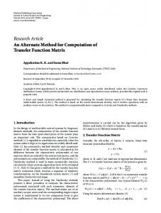
These expansions can then be inserted into (5.3) and (6.10) and the surface integrals over S ′ performed numerically to yield the desired expansion (2.8). Since the expansions (7.1) and (7.2) have been carried out analytically, the expansion (2.8) will be consistent with the conditions (6.16) and (6.17) even if the surface integrals are not done perfectly. The program just described has been implemented for the case of a bent rectangular box with straight end arms as illustrated in Figure 6.1 below (see Appendix B for a more detailed discussion of possible surface topologies, i.e., boxes, tori, etc., and associated choices of the orientation of the Dirac string). The volume V ′ enclosed by such a box is well suited to integrating reference trajectories and finding maps about these trajectories for the case of bending magnets. Preliminary results have been obtained for dipole-like fields that can be modeled analytically (e.g. fields produced by a superposition of magnetic monopoles located outside V ′ ). For these model fields surface normal fields and surface scalar potentials on S ′ can be calculated, and reference trajectories and their associated transfer maps can then be calculated using the expansion (2.8) obtained by integrating over S ′ . For these model fields, reference trajectories and transfer maps about them can also be obtained from the direct analytic expansion of the associated model vector potential. Numerical comparisons were made for fields computed in three ways: 1. directly from the sources outside of the surface, 2. by integrating the kernels (5.1) and (6.11) times source strengths over the surface, and 3. from expansions (like that of Eq. 2.8, but in three variables) obtained by integrating the derivatives of the kernels times source distributions over the surface. It was found that the vector potential and its derivatives computed by the three methods agreed well for points within V ′ . Correspondingly, it was found that the reference trajectories and their associated maps obtained by the two methods agreed well. For problems of actual interest the surface normal fields and surface scalar potentials on S ′ will be determined numerically by the use of some 3-dimensional field code or by direct measurement, and the surface integrals (5.3) and (6.10) over the expansions (7.1) and (7.2) will be carried out using these numerical values. Based on the test results obtained so far, there is every reason to believe that reference trajectories and their associated transfer maps computed from these surface data should be just as highly accurate as it was for the test cases. That is, by using the methods of this paper, modules can be added to existing electromagnetic codes that will produce reliably, when requested, associated transfer maps to any order for arbitrary static charged-particle beamline elements. Thus it should now be possible, for the first time, to design and analyze the effect of general static beam-line elements, including all fringe-field and error effects, in complete detail.

9

Figure 6.1. A volume V ′ consisting of a bent rectangular box with straight arms suitable for treating a bending magnet. The box encloses both the main bending field and the entry and exit fringe fields. The straight arms at the ends are sufficiently long that the surface normal field and surface scalar potential make negligible contributions on the entry and exit faces. Also shown is a sample reference trajectory that, as expected, is almost straight at the ends and bent in the middle.

8

Conclusions

A new method has been developed for the computation of charged-particle transfer maps for general fields and geometries based on the use of surface (boundary-value) data. The method requires a knowledge of all three field components on the surface (or, equivalently, the value of the normal field component and the scalar potential on the surface). These surface values are convolved with explicitly known and geometry-independent kernels to produce interior fields. The kernels themselves are obtained by the use of Helmholtz’s theorem and Dirac magnetic monopole vector potentials. The resulting interior fields satisfy the Maxwell equations exactly and are analytic functions of position even if the surface data contains errors and/or the convolutions are only performed approximately. Thus, the resulting transfer maps are expected to be optimally robust against computational and/or measurement errors. Using these methods, modules can be added to existing numerical electromagnetic field-solving codes that would produce reliably, when requested, associated transfer maps to any order for arbitrary static charged-particle beamline elements.

9

References

1. A. J. Dragt, “Lie Methods for Nonlinear Dynamics with Applications to Accelerator Physics”, University of Maryland Physics Department technical report, (2000), Section 1.6. 2. The Art and Science of Magnet Design: Selected Notes of Klaus Halbach, LBL Pub-755, Lawrence Berkeley Laboratory, Feb. 1995, p. 65. 3. M. Venturini and A. Dragt, “Accurate Computation of Transfer Maps from Magnetic Field Data”, Nucl. Inst. and Meth. A 427, pp. 387-392 (1999). 4 A. J. Dragt et al., MaryLie 3.0 amd 5.0 manuals, University of Maryland Physics Department technical reports, (2000). 5. P. L. Walstrom, private communication. 10

6. H. Wind, “Evaluating a Magnetic Field Component from Boundary Observations Only”, Nucl. Inst. and Meth. 84 (1970) pp. 117-124. 7. B. Hartmann, M. Berz, and H. Wollnik, “The Computation of Aberrations of Fringing Fields of Magnetic Multipole and Sector Magnets Using Differential Algebra”, Nuc. Inst. and Meth. A297 (1990) pp. 343-353. 8. M. Berz, Modern Map Methods in Particle Beam Physics, Vol. 108 of Advances in Imaging and Electron Physics, Academic Press, San Diego, 1999, pp. 132-144. 9. R. Plonsey, R.E. Collin, Principles and Applications of Electromagnetic Fields, The Maple Press Company, PA, 1961. 10. J. D. Jackson, Classical Electrodynamics, 3rd Ed., John Wiley and Sons, N.Y., 1999, p. 278. 11. J. Schwinger, L. DeRaad, et al., Classical Electrodynamics, Perseus Books, 1998, Chapters 2 and 30. 12. Ref. 1, Chapter 26. 13. Ref. 10, p. 36, Eq. 1.36.

Appendix A Sources on Surfaces of Rotation in Cylindrical Coordinates Sources on surfaces with rotational symmetry can be used to represent the fields in the special case of magnetostatic or electrostatic elements with a straight or slightly curved reference trajectory (e.g., quadrupoles or dipoles with small sagitta). A cylindrical coordinate system is the most convenient one to use in treating this case. Field-point coordinates in the following are denoted by (r, θ, z), and source coordinates by (a, φ, z ′ ). A toroidal surface that encloses the magnet and has a hole through which the beam pipe passes can be generated by rotating the appropriate closed space curve around some axis. A special case of this is an infinite cylinder, for which the space curve closes at infinity. It should be noted that in some accelerator applications, the beam pipe extends into the spaces between quadrupole pole pieces and encloses points with radial distances from the magnet axis that are larger than the pole-tip radius. In these cases, no single series-expansion map can represent the entire beam-pipe volume. If one is interested in a map for regions beyond the pole-tip radius, it is necessary to use an offset reference trajectory to ensure that the volume of interest is within the radius of convergence of the field expansion. The general space curve can be defined by two functions of arc length s or some other convenient curve parameter, i.e., a = A(s), z = Z(s). The sources can be represented by Fourier series in φ with coefficients that are functions of arc length s and the fields and potentials by Fourier series in θ with coefficients that are functions of r and z. As in the case of a general surface, the sources are a superposition of a fictitious single surface-charge distribution arising from the normal component of field at the surface and a fictitious double-layer distribution (i.e., normally-pointing surface dipole-density distribution) that arises from the tangential components of the field at the surface. In the even simpler case of an infinitely long cylinder, it is straightforward to find either a double-layer or single-layer distribution that alone represents the fields inside the cylinder (existing MARYLIE computer subroutines that treat this case were described in Section 3). If the surface does not touch real sources, distributions are continuous except at s values where the curve tangent is not continuous. The fictitious surface 11

charge distribution arising from the normal component of the field at the surface can be written in the form ∞ X B(s, φ) · n(s, φ) = fm (s) sin(mφ). (A.1) m=1

If the sources have no solenoidal component (i.e., no net current flows completely around the hole of the torus), m takes on the values m = 1, 2, 3, · · ·. The lack of terms with m = 0 will be assumed in the following. (In (A.1), the cosine terms are omitted for brevity. This corresponds to admitting only so-called normal multipole magnets. It is straightforward to add cosine terms if required by the symmetry of the problem). For a particular s value, each term in (A.1) corresponds to a sinusoidal charge ring of radius a(s) at axial position z ′ (s). The fictitious double-layer (surface dipole-density) distribution d that arises from the tangential field at the surface can be written in the form d(s, φ) = n(s, φ)ψ(s, φ).

(A.2)

As in the general three-dimensional case, the double-layer density is the magnetic scalar potential at the surface, i.e, ψ(s, φ) = Φ{r′ [(a(s), φ]}. If the scalar potential is to be obtained from measurements, it is suffficient, for example, to measure Bφ everywhere on the surface, but measure the tangential component of B perpendicular to Bφ along the surface for only one value of φ. The fictitious dipoledensity distribution arising from the tangential components of field at the surface can be written in the form ∞ X ψ(s, φ) = hm (s) sin(mφ). (A.3) m=1

The scalar potential for the mth term in (A.1) (the single-layer density distribution) is given by the following integral: I Z π cos mα sin mθ dα, (A.4) a(s)fm (s)ds Φm (r, θ, z) = 2π R 0 where

 1/2 R = a(s)2 + r2 + [z − z ′ (s)]2 − 2a(s)r cos α .

(A.5)

The integral over α in (A.4) can be expressed in terms of a Legendre function of the second kind, Z π  a(s)2 + r2 + [z − z ′ (s)]2  1 cos mα . (A.6) dα = p Qm−1/2 R 2a(s)r a(s)r 0 Eq. (A.4) then becomes

sin mθ Φm (r, θ, z) = 2π

I

 a(s)2 + r2 + [z − z ′ (s)]2  1 ds. a(s)fm (s) p Qm−1/2 2a(s)r a(s)r

(A.7)

The function of (A.6) times the sin mθ factor is the three-dimensional cylindrical analog of the line potential of two-dimension potential theory and is also logarithmically divergent as the field point approaches the source. It is the scalar potential of a ring of radius a(s) with a line charge density that varies as sin mφ. For points r, z close to a, z ′ , the potential varies as the logarithm of the distance times sin mθ. 12

For Hamiltonian dynamics calculations, a vector potential that gives the same fields as the scalar potential of (A.7) is desired. The vector potential for the mth term in (A.1) can be found by integrating the Dirac monopole expressions over the surface. However, simpler expressions for the vector potential can be obtained (this amounts to a gauge transformation of the Dirac monopole expressions) directly from the scalar potential in a gauge with Aθ = 0 by equating the magnetic field components from the gradient of (A.7) to the field components from the curl of the vector potential. Simple integration over θ gives the two vector-potential components Ar and Az :

Arm (r, θ, z)

r cos mθ =− 2mπ

I

a(s)fm (s)

and Azm (r, θ, z) =

r cos mθ 2mπ

I

a(s)fm (s)

 a(s)2 + r2 + [z − z ′ (s)]2 i 1 ∂ h p ds, Qm−1/2 ∂z 2a(s)r a(s)r

 a(s)2 + r2 + [z − z ′ (s)]2 i ∂ h 1 p ds. Qm−1/2 ∂r 2a(s)r a(s)r

(A.8)

(A.9)

The derivatives in the above expressions can be evaluated explicitly using the derivative relations for Legendre functions, and the chain rule. The Legendre functions themselves can be computed for large arguments by recursion with the complete elliptic integrals K and E with the appropriate arguments, and for small arguments from the hypergeometric series expressions1 . The scalar potential for the mth Fourier component of the fictitious surface dipole-density sources arising from the tangential field components at the surface (see (A.3)) can also be expressed in terms of Legendre functions: I  a(s)2 + r2 + [z − z ′ (s)]2 i  ∂ sin mθ ∂ h 1 p Qm−1/2 Φm (r, θ, z) = ds. − zˆ a(s)hm (s)n · a ˆ 2π ∂a ∂z 2a(s)r a(s)r (A.10) In (A.10) , a ˆ is a radial unit vector and zˆ an axial unit vector. The vector-potential components are again obtained in a gauge with Aθ = 0 by equating the gradient of the scalar potential to the curl of the vector potential, and integrating over angle. The result is I  ∂2  a(s)2 + r2 + [z − z ′ (s)]2 i r cos mθ ∂ 2 h 1 Arm (r, θ, z) = − −ˆ z 2 p a(s)hm (s)n· a ˆ ds, Qm−1/2 2mπ ∂a∂z ∂z 2a(s)r a(s)r (A.11) and I  ∂2  a(s)2 + r2 + [z − z ′ (s)]2 i 1 ∂ 2 h r cos mθ z p ds. −ˆ z a(s)hm (s)n· a ˆ Qm−1/2 Am (r, θ, z) = 2mπ ∂a∂r ∂z∂r 2a(s)r a(s)r (A.12) For series expansion of the potentials and fields around the axis, which is needed for numerical map generation, Dougall’s integral expression2 with the on-axis generalized gradient is used to extend the potential to non-zero values of r. Given the mth Fourier component of the scalar potential Vm in cylindrical coordinates, we first note that the leading behavior of Vm (r, z) with r near the axis is Vm ∼ rm , and then define the on-axis generalized gradient to be gm (z) = lim

r→0

mVm (r, z) . rm

13

(A.13)

(In A.13, the factor of m is included to make gm consistent with the usual definition of quadrupole gradient for m = 2). Dougall’s integral expression is Z π (m − 1)!rm Vm (r, z) = gm (z + ir cos t) sin2m tdt. (A.14) Γ(m + 1/2)Γ(1/2) 0 The series expansion for Vm near the axis is obtained by replacing gm (z + ir cos t) by its Taylor expansion, with ir cos t as the expansion parameter, and integrating term by term. The imaginary terms integrate to zero, leaving the well-known series expansion Vm (r, z) = (m − 1)!rm

∞ X

 r2 d2 n 1 gm (z) − n!(n + m)! 4 dz 2 n=0

(A.15)

For the particular case of Legendre-function expressions of (A.6)-(A.12), the hypergeometric- function representation for Qm−1/2 is used to find their limiting behavior with r near the axis [i.e., evaluate the limit of (A.13)]. The series expansion for the Legendre-function factor (A.6) is then found to be  a(s)2 + r2 + [z − z ′ (s)]2  1 p = Qm−1/2 2a(s)r a(s)r ∞  r2 d2 n 1 1 πam rm (2m − 1)!! X − m+1/2 .  2 2m n!(n + m)! 4 dz 2 a + [z − z ′ (s)]2 n=0

(A.16)

The series expansions for the scalar and vector potentials are then obtained by substituting the right-hand side of (A.16) for the quantity  a(s)2 + r2 + [z − z ′ (s)]2  1 p Qm−1/2 2a(s)r a(s)r

(A.17)

everywhere it occurs in (A.7)-(A.12). For numerical evaluation of the series coefficients as a function of z, in general it is necessary to first obtain the Fourier coefficients for the scalar and dipole densities as a function of s and then perform the integrals inside the summation sign over s by numerical quadrature. It is possible to perform the integrals analytically if Fourier coefficients of the source densities are represented as piecewise-continuous polynomials in s. Finally, in reference to the problem of fitting three-dimensional field data on or near the axis in straight-axis systems and extending it outward in radius (a mathematically unstable procedure, which the surface-data method of this paper avoids), one could first Fourier-analyze the data in azimuthal angle, and treat each Fourier component as a separate fitting problem in r and z using the appropriate derivatives of the mth component of (A.15) times sin mθ or cos mθ, together with a trial function for gm (z). One might, for example, represent gm (z) by high-order (5th or higher) splines and find the spline coefficients by fitting fields from (A.15) to field values specified on a surface or over a volume. The series of (A.15) will end at a finite value of n with this representation of gm because splines are made up of piecewise-continuous polynomials of finite order, while the “true” gm is infinitely differentiable. This representation therefore can model only the lowest-order behavior of the field, for points at relatively small distances from the axis relative to the physical aperture of the element. Other methods, in which transcendental functions are used to represent gm , give a series that does not truncate, but the improvement can be illusory because the higher 14

derivatives and the associated higher-order terms can be wrong, and in many cases, wildly wrong. The fundamental problem is that the fitting function that represents gm is generally not the “true” function and if it has simple poles, the poles, which represent sinusoidal ring sources, have little to do with the “true” sources.

References (Appendix A) 1. M. Abramowitz and I. Stegun, Ed., Handbook of Mathematical Functions, Dover Publications, NY , 1972 (a reprint of the NBS #55, Applied Mathematics Series of 1964 with the same title), pp. 331-337. 2. E. T. Whittaker and G. N. Watson, A Course of Modern Analysis, Fourth Edition (reprinted), Cambridge University Press, 1963, p. 400.

Appendix B Surface Topologies and Dirac Monopole Orientation Various surfaces in addition to the curved box and infinite cylinder already discussed can be considered. For example, toroidal surfaces of the type shown in Fig. B.1 can be made to have minimal clearance of the magnetic element on the ends and have a hole that is large enough to accomodate the beam pipe. Since the beam goes through the hole, and not through the surface, the two ends of the surface do not need to extend out to field-free regions and the surface can be shorter. Also, if the vertical surfaces at the ends are made to extend far enough out to the sides that the fields on them become negligible at the outer edges, source strengths on the outside surfaces connecting them are negligible. In such a case source distributions need only be found for inner surface around the hole and for the parts of the vertical end surfaces near the ends of the hole. In most cases, all of the pieces of the surfaces can be constructed from flat pieces and parts of cylindrical surfaces. For example, for curved dipoles, the vertical parts of the inner surface could be made of segments of cylinders.

15

AAAAAA AAA AA AAAAAA AAA AA AAAAAA AAAAAA AAAAAA AAAAAA AAAAAA b

a

Fig. B.1 Two possible toroidal surfaces with Dirac string orientations indicated. Surface a would be used with an H magnet, while b would be used with a quadrupole. It should be noted that the discontinuities in the tangents to the surface are not a problem in principle because the surfaces are fictitious and have vacuum on each side; the is no field peaking as there is at the edge of a magnet yoke, etc. However, attention must be paid to numerical problems related to discrete source placement and spacing along edges. It can be seen that if toroidal surfaces are used, use of Dirac monopoles with strings perpendicular to the end surfaces could be a problem in curved beamlines, as they could intersect the beam volume. This problem can be avoided by using strings tangential to the surface as shown in Fig. B.1. If tangential strings are used, a two-sided Dirac monopole with two half-strength strings going in opposite directions can be used; the associated expression for the vector potential is somewhat simpler and may have some advantages in computation: Gn (r; r′ , m) =

m × (r − r′ ) . 4π|m × (r − r′ )|2

16

(B.1)