Computation of Turbulent Free-Surface Flows ... - Semantic Scholar

Computation of Turbulent Free-Surface Flows Around Ships and Floating Bodies

Vom Promotionsausschuß der Technischen Universität Hamburg-Harburg zur Erlangung des akademisches Grades Doktor-Ingenieur genehmigte Dissertation

von

Rodrigo Azcueta Repetto aus Argentinien

2001

Gutachter: Prof. Dr.-Ing. M. Perić Prof. Dr.-Ing. E. Kreuzer

Mündliche Prüfung: 5.07.2001

Contents Nomenclature

v

1

. . . .

1 1 2 5 6

. . . . . . . . . . .

9 9 11 11 14 15 15 16 17 20 22 24

. . . . . . . . . . . .

25 25 26 27 28 28 31 33 34 37 40 41 47

2

3

Introduction 1.1 Motivation . . . . . . . . 1.2 Previous Related Studies 1.3 Present Contributions . . 1.4 Outline of the Thesis . .

. . . .

. . . .

. . . .

. . . .

. . . .

. . . .

. . . .

. . . .

. . . .

. . . .

. . . .

. . . .

. . . .

Numerical Method 2.1 Methodology . . . . . . . . . . . . . . . . . . . 2.2 Outline of the RANSE solver . . . . . . . . . . . 2.2.1 Basic Method . . . . . . . . . . . . . . . 2.2.2 Free-Surface Method . . . . . . . . . . . 2.3 Coupling Fluid Flow and Rigid Body Motion . . 2.3.1 Frames of Reference . . . . . . . . . . . 2.3.2 Equations of Motion of the Rigid Body . 2.3.3 Integration of the Body Motion Equations 2.3.4 Definition of the Rotation Angles . . . . 2.3.5 Boundary Conditions . . . . . . . . . . . 2.3.6 Coupling Algorithm . . . . . . . . . . .

. . . .

. . . . . . . . . . .

. . . .

. . . . . . . . . . .

. . . .

. . . . . . . . . . .

. . . .

. . . . . . . . . . .

. . . .

. . . . . . . . . . .

Steady Free-Surface Flows Around Ships 3.1 Introduction . . . . . . . . . . . . . . . . . . . . . . . . . 3.2 Grid Generation . . . . . . . . . . . . . . . . . . . . . . . 3.3 Boundary and Initial Conditions . . . . . . . . . . . . . . 3.4 Test Cases . . . . . . . . . . . . . . . . . . . . . . . . . . 3.4.1 Wigley Hull . . . . . . . . . . . . . . . . . . . . . 3.4.2 Series 60 Hull . . . . . . . . . . . . . . . . . . . . 3.4.3 Other Test Cases . . . . . . . . . . . . . . . . . . 3.5 Dependence of Friction Resistance on Grid Quality . . . . 3.6 Effects of Time Step on Resistance . . . . . . . . . . . . . 3.7 Strategy for Best Convergence . . . . . . . . . . . . . . . 3.8 Influence of Discretisation Scheme on Pressure Resistance 3.9 Concluding Remarks . . . . . . . . . . . . . . . . . . . . iii

. . . .

. . . . . . . . . . .

. . . . . . . . . . . .

. . . .

. . . . . . . . . . .

. . . . . . . . . . . .

. . . .

. . . . . . . . . . .

. . . . . . . . . . . .

. . . .

. . . . . . . . . . .

. . . . . . . . . . . .

. . . .

. . . . . . . . . . .

. . . . . . . . . . . .

. . . .

. . . . . . . . . . .

. . . . . . . . . . . .

. . . .

. . . . . . . . . . .

. . . . . . . . . . . .

. . . .

. . . . . . . . . . .

. . . . . . . . . . . .

CONTENTS

iv 4

5

6

Computation of the Ship’s Running Attitude 4.1 Introduction . . . . . . . . . . . . . . . . 4.2 Series 60 Hull . . . . . . . . . . . . . . . 4.3 Blunt-Bow Ship Model (Breaking Waves) 4.3.1 Model-Fixed Computations . . . 4.3.2 Model-Free Computations . . . . 4.4 Concluding Remarks . . . . . . . . . . .

. . . . . .

49 49 50 58 59 63 67

. . . . .

69 69 70 79 83 88

Conclusions and further work 6.1 Summary and Conclusions . . . . . . . . . . . . . . . . . . . . . . . . . . 6.2 Further Work . . . . . . . . . . . . . . . . . . . . . . . . . . . . . . . . .

91 91 94

. . . . . .

. . . . . .

Freely-Floating Bodies 5.1 Introduction . . . . . . . . . . . . . . . . . . 5.2 Drop Tests (Plane Motion) . . . . . . . . . . 5.3 Boat Section (Plane Motion) . . . . . . . . . 5.4 Sailing Boat in Planing Condition (3-D Case) 5.5 Concluding Remarks . . . . . . . . . . . . .

. . . . . .

. . . . .

. . . . . .

. . . . .

. . . . . .

. . . . .

. . . . . .

. . . . .

. . . . . .

. . . . .

. . . . . .

. . . . .

. . . . . .

. . . . .

. . . . . .

. . . . .

. . . . . .

. . . . .

. . . . . .

. . . . .

. . . . . .

. . . . .

. . . . . .

. . . . .

. . . . . .

. . . . .

. . . . . .

. . . . .

. . . . . .

. . . . .

A CD with Animations

97

Bibliography

99

Curriculum Vitae

105

Nomenclature Roman Symbols

[m] [1] [1] [1] [1] [1] [1] [1] [1] [1] [1] [1] [m] [1] [N] [N] [N] [N] [m/s ] [1] [1] [kg m ] [kg m ] [kg m ] [kg m ] [kg m ] [kg m ] [1] [kg m ] [1] [1] [1] [m /s ] [m]

Beam of ship Volume fraction Block coefficient Local skin friction coefficient Frictional resistance coefficient Yaw moment coefficient Courant number Local pressure coefficient Pressure resistance coefficient Residuary resistance coefficient Total resistance coefficient Sway force coefficient Depth of ship Froude number Total force acting on the body expressed in the Newtonian RS External forces acting on the body expressed in the Newtonian RS Fluid force acting on the body expressed in the Newtonian RS Towing force acting on the body expressed in the Newtonian RS Vector acceleration of gravity Unit vector defining the -axis Absolute time derivative of Roll moment of inertia about axis Pitch moment of inertia about axis Yaw moment of inertia about axis Product of inertia for

axes Product of inertia for axes Product of inertia for axes Unit vector defining the -axis Tensor of inertia of the body about the ( ) axes Unit vector defining the -axis

Absolute time derivative of Unit vector defining the -axis Kinetic energy of turbulent fluctuation per unit mass Roll radius of gyration about axis v

NOMENCLATURE

vi

! ! " " # $

[m] [m] [1] [1] [m] [1] [m] [m /s] [kg] [N m] [N m] [N m] [1] [N/m ] [1] [m ] [m ] [m ] [s] [s] [s] [1] [m/s] [m/s] [m/s] [m ] [N] [m] [m] [m] [m] [m/s]

Pitch radius of gyration about axis Yaw radius of gyration about axis Unit vector defining the -axis

Absolute time derivative of Centre of gravity above keel Unit vector defining the -axis Reference length of ship Kinematic viscosity Body mass Total moment acting on expressed in the Newtonian RS Hydrodynamic moment acting on expressed in the Newtonian RS External moment acting on expressed in the Newtonian RS Unit normal vector at CV-surface Total pressure Reynolds number ( ) CV total surface Wetted hull area at rest CV face area Time Initial time instant Roll period Transformation matrix from the body-fixed RS into the Newtonian RS Ship (model) speed Fluid velocity vector CV-surface velocity vector CV-volume Ship (model) weight force Longitudinal coordinate in the body-fixed RS Towing force attachment point expressed in the body-fixed RS Longitudinal coordinate in the Newtonian RS Centre of gravity expressed in the Newtonian RS Linear velocity of expressed in the Newtonian RS

[m/s ] [m]

Linear acceleration of expressed in the Newtonian RS CV face centres expressed in the Newtonian RS

[m] [m] [m] [m] [1] [m] [m]

Velocity of CV face centres expressed in the Newtonian RS Towing force attachment point expressed in the Newtonian RS Transverse coordinate in the body-fixed RS Transverse coordinate in the Newtonian RS Dimensionless distance from the wall Vertical coordinate in the body-fixed RS Vertical coordinate in the Newtonian RS

vii Greek Symbols

% Æ

[Æ ] [1] [N] [m] [s] [m] [m] [m] [m /s ] [kg/(ms)] [kg/(ms)] [Æ ] [Æ ] [kg/m ] [N/m ] [m /s ] [Æ ] [rad/s]

Yaw or drift angle Logarithmic decrement of rolling Displacement force Grid spacing normal to the hull surface Size of time step Grid spacing in -direction Grid spacing in -direction Grid spacing in -direction Dissipation per unit mass Molecular viscosity Eddy viscosity Roll or heel angle Yaw or course angle Fluid density Tangential stress acting on CV face Reynolds stress tensor Pitch or trim angle Angular velocity expressed in the Newtonian RS

[rad/s ]

Angular acceleration expressed in the Newtonian RS

!

& ' ' ( ) * + + ,

Acronym CDS CFD RS CVs

DOF

GIS HRIC

-

RANSE UDS

Central Differencing Scheme Computational Fluid Dynamics Reference system Control Volumes Delay Factor for body velocity Degrees Of Freedom Centre of gravity of the vessel Grid Independent Solution High-Resolution Interface-Capturing Scheme Origin of the Newtonian RS Reynolds Averaged Navier-Stokes Equations Upwind Differencing Scheme

Remarks: whenever possible ITTC (1999) symbols and terminology were used. Symbols and acronyms not included in this list are defined in the text.

viii

NOMENCLATURE

Chapter 1 Introduction 1.1 Motivation The long-term vision in numerical ship hydrodynamics is to simulate the behaviour and performance of full scale ships under real operating conditions, and in this way to get rid of tank tests and their uncertainties in the model-ship correlation and other limitations such as costs and delivery time. The numerical methods should be able to predict ship performance en route, ship manoeuvrability in open and restricted waters as well as ship behaviour in waves. For ship performance en route the required delivered power at the propeller is important. This depends on the ship resistance in the steady-state sailing condition and on the propeller-hull interaction. The task of Computational Fluid Dynamics (CFD) in this matter would be to simulate the full scale propulsion test, including all resistance components (viscous, wave, wind, etc.) and the unsteady propeller flow. Ship manoeuvring is still a more complicated task: the propeller-rudder-hull interaction has to be taken into account and the computations have to be able to handle a highly turbulent asymmetrical flow over the hull, boundary layer separation and re-attachment as well as complicated wave patterns. Ship behaviour in a seaway is important from the point of view of ship safety, as well as with regard to added resistance in waves and thus sustained speed. A big challenge in numerical ship hydrodynamics is to accurately simulate the ship manoeuvring in waves including all non-linearities and viscous effects. At which stage we are on the path towards fulfilling the long term vision and which simplifications have to be accepted to this date will be the topic of this introduction. Since at present and in the foreseeable future it is impossible to achieve these ambitious goals with one single numerical method, so far the general approach has been to split the task in separate sub-problems and solve them by means of different methods. The motivation of this work is to go a step further into some of these sub-problems, in particular when it comes to accurately predict the ship performance including the most important resistance components, and in paving the way for viscous flow simulations of freely-floating body motions in six degrees of freedom. In the tasks mentioned above, the free-surface deformation and the ship’s running attitude have to be included in the simulations. Sometimes the viscosity and the turbulence of the fluid play a crucial role and have to be taken into account as well. This is the case in manoeuvring, where the rotational effects, which are viscous in nature, dominate, and in roll motions, where the viscous damping is important. This thesis deals with the application and extention of a flow solver to “Computations of Turbulent Free-Surface Flows Around Ships and Floating Bodies”. 1

2

CHAPTER 1. INTRODUCTION

1.2 Previous Related Studies The following description of the state-of-the-art in ship hydrodynamics does not pretend to be exhaustive, but it can be regarded as being representative of the main advances in this field in recent years. The state-of-the-art in ship hydrodynamics is mirrored in part by the international journals and the main conferences in this field, such as the Symposium on Naval Hydrodynamics and the International Conference on Numerical Ship Hydrodynamics, both of which are held alternately every second year, as well as the Workshops on CFD in Ship Hydrodynamics, which has recently focused on viscous flow computations. As our interest lies in freely-floating ships, we will concentrate in the following on developments which are relevant to this kind of simulations. The starting point for simulations of floating bodies – steady or unsteady –, is the computation of free-surface flows, since the bodies considered have to be suspended – in equilibrium or not – at the interface between the two fluids, air and water. At the CFD Workshop in Gothenburg in 1990 all free-surface codes were based on potential flow, while RANSE (Reynolds Averaged Navier-Stokes Equations) solvers were confined to stern/wake flows. However, more and more researchers worldwide are coming to the conclusion that the future belongs to free-surface RANSE solvers, even those who originally developed potential flow codes. For practical ship design purposes, most wave resistance computations neglect viscosity effects and most viscous flow computations still neglect wave making and compute the double-body flow. Researchers around the world however increasingly recognise the need for predicting all components of the ship resistance by means of a single code, taking into account the coupling and non-linear effects. The first viscous free-surface computations date back longer than thirty years ago and were based on the so-called interface-capturing technique. They were confined to relatively simple cases and mostly to internal flows, such as sloshing in a tank. The real breakthrough in viscous free-surface computations for ship flows came with the CFD Workshop in Tokyo in 1994, where ten methods included this feature. However, with the exception of one method, Kodama et al. (1994), all others used the interface-tracking technique (so-called movinggrid methods), in which the grid is fitted to the free surface and follows its shape as the waves deform. A few years later, the moving-grid methods started to show their limitations, as they were not adequate to handle complex ship geometries and overturning waves. Interface-capturing methods of the VOF type (Volume Of Fluid) and its variations (also the akin level-set technique) were then “rediscovered” for ship flows and implemented into many codes, among others into the program COMET, which is used in this work. They soon proved to be superior for handling strong non-linearities and are today the most obvious choice for computing complex free-surface shapes with breaking waves, sprays and air trapping, which are often encountered in ship hydrodynamics. In this way, the resistance component which is due to wave formation and its interaction with the viscous resistance can be quantified with better accuracy than by using potential flow panel methods. However, the major problem with RANSE free-surface methods (apart from turbulence modelling) is still resolution, but this obstacle will inevitably be overcome some time in the future. Another advantage of some methods of VOF type is that they can compute the air flow as well, and in this way determine the wind resistance of the upper hull and superstructure and the wind-over-deck conditions for helicopter landing or funnel smoke tracing. For a good description of the evolution of free-surface methods see Larsson et al. (1998). In order to yet improve resistance predictions further, the ship’s running attitude, i.e. the

1.2. PREVIOUS RELATED STUDIES

3

dynamic sinkage and trim (and eventually heel) of the ship underway should be included in the computations, since its effect is usually significant. For ships sailing in shallow or restricted waters this issue is of great importance, since the ship’s safety may be endangered. Resistance tests in towing tanks can either be in the so-called model-free or the model-fixed condition, depending if the model is free to change its running attitude or not, respectively. CFD computations have also adopted this classification, as they have to be validated by the corresponding tank tests. So far, computations in the model-free condition have been confined to potential flow panel methods. Viscous flow computations to this date are in the model-fixed condition, either at the floating attitude at rest or at the running attitude measured in the towing tank. In the first case, they do not include the difference in resistance due to the change in running attitude, which is usually significant. In the second case, they cannot be considered as a resistance prediction but rather as a validation of computed with measured values. At the 1994 CFD Workshop all nine free-surface viscous flow computations presented (benchmark test with the Series 60 model) were limited to the hull fixed in trim and sinkage. The organisers of the last CFD Workshop, which was held in Gothenburg in September 2000, had intended to include the computation of the ship’s running attitude for one of the benchmarks (viscous free-surface flow around a container ship) in the programme. This request, however, was withdrawn some time after it had been announced. In the author’s opinion, this was because no research group was able to deliver such an analysis at the time. The ship’s running attitude has usually been neglected even in research applications. Exceptions are found with Orihara and Miyata (1997) who computed the sinkage and trim of semi-planing boats, and with Miyata et al. (1997) who computed the sinkage, trim and heel of sailing boats. Both contributions used deformable grids. The Japanese researchers, mostly at the Tokyo University around Prof. Miyata, have been very active in innovating all areas of numerical ship hydrodynamics, and have often presented some applications many years before other groups around the world. Not only the determination of the dynamic position afloat but also the accurate modelling of ship motions in six degrees of freedom can be done with a single code by coupling the rigid body dynamics, given by the equations of motion of the rigid body, with the solution of the flow field around the hull computed by a RANSE solver. However, the state-of-theart in viscous simulations of ship slamming, water on deck, manoeuvring and motions in waves is to decouple the problem into two ones: 1. The determination of the ship motion, which is done beforehand by non-linear ship motion programs based on potential flow or is taken over from model tests; 2. The actual viscous flow simulation with the prescribed forced motion. Single-code simulations of manoeuvring and sea-keeping are mostly limited to potential flows and require a considerably greater effort than steadily advancing ships, and have several limitations. In manoeuvring, when viscous effects are to be taken into account, the general approach is to solve the flow around the bare hull advancing steadily with a yaw angle or performing a turn-circle, and to solve separately the flow around the appendages and the propeller, and then provide a ship motion simulation program with these forces. In this way, the inaccurate empirical force coefficients gained from analytical approaches, potential flow or regression analysis of tank tests are substituted. This approach was followed for instance by Sato et al. (1998), Cura Hochbaum (1998), Alessandrini and Delhommeau (1998) and Ohimori et al. (1998). For a good review on this topic see Landrini (1999). Single-code RANSE time simulations of manoeuvring ships have been attempted for example by Miyata et al. (1997)

4


and Akimoto and Miyata (1999) for sailing boats in rudder-induced tacking motions and by McDonal and Whitfield (1996) for a submarine with a rotating propeller (no free surface) and by Takada et al. (1999) for the forced motion of the keel of a racing yacht and for an underwater vehicle with controllable lifting surfaces (both without free surface). State-of-the-art for ships in waves are the three-dimensional, fully non-linear potential flow methods (boundary-integral-equation methods (BIEM), Green-function methods and Rankine source methods), which can simulate the motion of freely-floating bodies interacting with waves. These methods, however, show a number of limitations and complications, such as: absence of viscosity, problems with strong non-linearities and forward speed, and large computational effort. The development of these methods (see Berkvens (1998) for a good description of this evolution) began with the computation of the relatively simple twodimensional linearised problem of radiation (forces on the body oscillating in calm water) and diffraction (forces on the fixed body in regular waves), which delivered the added mass and damping coefficients to be then extended to the 3-dimensional hull by strip methods. The solutions were then gradually refined, from linear to fully non-linear, from 2-D to 3-D, from frequency to time domain, and from forced motions (radiation/diffraction problem) to freely-floating bodies, first in two (heave and pitch) and finally in six degrees of freedom. RANSE methods for ships in waves and related problems undergo a similar evolution concerning the number of space dimensions, forced or free motions, laminar or turbulent and viscous or inviscid (EULER methods). Forced motion of bodies at a free surface were investigated, using RANSE or EULER methods, by: 1. By Schumann (1998) and Sames et al. (1998) for slamming investigations with 2-D bodies, and by Muzaferija et al. (1998) with a 3-D ship bow; 2. By de Jouëtte et al. (1999) for the forced roll motion of the Series 60 model at forward speed with the Euler equations and a VOF method, and by Gentaz et al. (1999) for the forced heave and pitch motions (decoupled) of the Series 60 model at forward speed with a moving-grid method for the free surface. Examples of computations for the diffraction problem were presented by Wilson et al. (1998) for a fixed steadily advancing naval combatant in regular head waves and by Rhee and Stern (1998) for the Wigley hull. First applications of freely-floating ships with a single viscous code are beginning to appear, for example, with the computations by de Jouëtte et al. (1999) for a 2-D freely heeling rectangle under a current (Euler equations), and as the most advanced contribution in my opinion the computations by Kinoshita et al. (1999) for the coupled heave and pitch motion of the Series 60 hull and the Wigley hull advancing in small and large regular head waves, respectively, solving the Euler equations. The last method uses a hybrid grid system of chimera type, finite difference discretisation and a moving-grid method for the free surface. They state that the advantages of such simulations compared to potential flow solutions are the generality of a single code approach which can include the viscous effects (viscous damping at resonance frequencies) and forward speed, delivering the same degree of accuracy at a similar computational effort. Developments for combining RANSE solutions in the region near the hull and linear potential flow solutions in the far field to solve the sea-keeping problem and the shore washing problem are very interesting and a matter of active research work. Examples of such hybrid methods were presented by Guillerm and Alessandrini (1999) and Yang et al. (1999) using a Fourier-Kochin approach to couple both methods for ships advancing in calm water. Both use moving-grid methods for the free surface. The first group uses RANS equations and the second group Euler equations and finite-element discretisation.

1.3. PRESENT CONTRIBUTIONS

5

1.3 Present Contributions The present work pursues three aims: The first one is to assess the accuracy of these freesurface RANSE computations for predicting the resistance of a ship advancing at constant speed in calm water. The second one is to extend the existing flow solver package COMET to allow the computation of the dynamic sinkage and trim (and eventually heel) of the ship underway, with the aim of improving the resistance prediction by considering the difference in resistance which arises when the ship changes its running attitude. The third one is to extend the method in such a way as to allow the time-accurate simulation of the motions of bodies floating freely at the free surface, i.e. in the six degrees of freedom. A further requirement for this work was to implement the coupling of the body motions and the fluid flow in such a way that any type of analysis, such as the ship resistance in the model-fixed or model-free condition as well as freely-floating bodies striving for an equilibrium position or interacting with external forces, could be performed by the same program by simply adjusting the appropriate parameters. Furthermore, the method should be extensible to still more complex tasks, such as those encountered in ship manoeuvring and in ships in waves. The present work was begun in 1996 with the first computations using the existing code COMET for real ship geometries under oblique flow conditions. With these computations, the main difficulties lie in the generation of high quality body-fitted and unstructured grids for a complex hull shape with appendages. This was essential for capturing the principal flow features of that complicated oblique flow. Those were still double-model computations, i.e. the free surface was idealised as a symmetry plane, see Azcueta (1996). Then, a VOFtype method was implemented in the code COMET, and the author carried out the early tests and validation of those free-surface computations for complex three-dimensional ship flows. Some of the results of that work are documented in Azcueta et al. (1997) and Azcueta et al. (1998). Central aspects of that work were the correct choice of boundary conditions and parameters of the numerical method as well as the validation of the results with towing tank data and with already successful computations of moving-grid type. After this test phase, it was evident that the potential of the VOF approach as implemented in the code COMET surpassed the existing interface-tracking methods by far. Breaking waves, sprays, air trapping, etc. could be handled, and no problems occurred with the adaptation of the free surface to the model geometry, regardless of how complex the geometry was. The computational effort was very similar to that of the moving-grid method. The clear advantages of the VOF method for these type of problems were documented in Azcueta et al. (1999a) and Azcueta et al. (1999b). As grid quality was essential for obtaining good results, a great effort was made to improve the grid generation process, and all kinds of topologies and distribution of grid points were studied. The work continued with the quantification of the sensitivity of the computed friction and pressure resistance to the grid quality and the variation of parameters of the numerical method and type of boundary conditions, as well as with a proposal for a novel type of extrapolation to grid-independent solutions for some of the computed variables. This work was published by Azcueta (2000). Building upon this experience, the method was extended to compute the body motions in six degrees of freedom. For this purpose, the rigid body motion equations were implemented within the framework of the flow solver COMET as a user-programmed module, which is linked and run simultaneously with the flow solver. With this feature, two new types of analyses were at hand. The first one was the determination the dynamic sinkage, trim and

6


heel, which is essential for improving the ship resistance prediction by taking into account the difference in resistance which arises when the ship changes its running attitude. In this way, the simulation of the model-free condition was made possible. The second type of analysis was the time-accurate simulation of freely-floating body motions. The ultimate aim of such investigations is to study the manoeuvrability and the behaviour of the ship in a seaway. But since this goal is still difficult to achieve for the time being due to the limited performance of computers, first applications of this feature were the simulation of the body responses when the bodies were released from a position out of equilibrium. As we have seen in the description of previous related studies, simulations like the ones to be presented here for ships floating freely at the free surface and including strong nonlinearities, viscous effects, forward speed, air and wave breaking resistance, etc. are not common at the moment. Rather they are among the first ones to be presented so far.

1.4 Outline of the Thesis The numerical approach implemented into the framework of the flow solver COMET for coupling the body motions with the fluid flow is introduced in Chapter 2. The first section of that chapter outlines different strategies for this task and describes the one chosen in this work, addresses some pros and cons, and introduces the most common methods for computing free surfaces. Then, the basic flow solver method is explained briefly, with an emphasis on the volume fraction method used for computing free surfaces. The remainder of Chapter 2 describes the strategy implemented for coupling the body motions with the fluid flow, beginning with the definition of the frames of reference used, followed by the introduction of the equations of motion of the rigid body and their integration in time, the calculation of forces and moments on the body, and some particularities of the strategy chosen, such as the definition of the rotation angles of the ship and the new required boundary condition on the body and at the outer flow-boundaries. Finally, an overview of the whole strategy is given. The remainder of the thesis is dedicated to the analysis of the performance of the numerical approach implemented. Examples of applications for both steady and unsteady flows around floating bodies at the free surface are presented. The analysis is organised in three parts, comprising Chapters 3, 4 and 5. The first part is concerned with the ship resistance prediction. Particularly the question concerning the achievable accuracy of the classical resistance tests simulated with this method – including the free surface – is addressed. One crucial point hereby is the validation with existing model tests, and an analysis of the influence of some numerical parameters on the results obtained. First, the grid generation procedure is explained, followed by the general boundary and initial conditions which apply to most computations in this work. Then, the benchmarks employed to validate the numerical resistance tests are presented. These are the Wigley hull, the Series 60 hull, a modern container vessel, and a two-dimensional hydrofoil with laminar-flow profile. Following this, three particularities of the computations are analysed. The first one is concerned with the grid quality and its resolution at the body wall, which is crucial for obtaining an accurate friction resistance prediction. The second one is the size of the time step required for the time integration and its influence on both pressure and friction resistance. The third one is

1.4. OUTLINE OF THE THESIS

7

the type of discretisation scheme used for the momentum equations and its influence on pressure resistance prediction. At this stage, a novel type of extrapolation procedure for obtaining near grid-independent solutions for pressure resistance without computing on extremely fine grids is proposed. In Chapter 4 the numerical approach is evaluated with respect to its suitability for calculating the dynamic sinkage, trim and heel of ships sailing at constant speed in calm water. The aim of such computations is to improve the resistance prediction by considering the difference in resistance, which arises when the vessel underway changes its running attitude. Two test cases are presented: The already used Series 60, and the model of a very fat ship with a blunt bow. In the first case, the straight-ahead sailing condition as well as a drift condition at a small yaw angle are computed and the results are validated with experimental data. In the second case the emphasis is on the large changes in running attitude and thus resistance, as well as on the bow-wave breaking pattern and its comparison with model tests. The main goal of Chapter 5 is to show the robustness and flexibility of the numerical approach for accurately modelling the general motions of bodies floating freely at the free surface. Three application cases are presented. All simulate the response of the body when released from a position out of equilibrium. The first one is the simulation of two-dimensional drop tests with a wedge. This case is used to validate the method with existing experimental data as well as to study the influence of some parameters of the numerical method such as time step and number of iterations on the dynamic response of the wedge. The second case is the two-dimensional large amplitude roll motion of the mid-ship section of a sailing boat. Two configurations are investigated – the bare hull and the hull with a fin keel – and the effects of the keel on the damping coefficient and thus on the roll motion are quantified. The third application is an extention of the last one to three dimensions and forward speed. The resulting configuration is a hull undergoing a coupled roll, pitch, sway and heave motion at high speed until reaching a planing condition. The goal of this application is to show how both the computation of the steady-state sailing attitude of a ship and the time-accurate simulation of freely-floating body motions can be performed with the same computer program by adjusting the appropriate parameters of the numerical method. The last chapter summarises the entire work, draws some conclusions and gives recommendations for improvement and further research work.

8


Chapter 2 Numerical Method This chapter describes the numerical approach implemented for both computing the freesurface flow around ships including their running attitude and simulating the motions of freely-floating ships. Firstly, different possibilities for coupling the body motion equations with the fluid flow equations – the Navier-Stokes equations – are mentioned and the one implemented in this work is described. Then, a brief outline of the Navier-Stokes solver COMET is given, whereby the emphasis lies on the interface-capturing method used to compute the distortion of the free surface. Starting point for simulations of floating bodies – steady or unsteady –, is the calculation of free-surface flows, since the bodies considered have to be suspended – in equilibrium or not – at the interface between the two fluids, air and water. The flow solver package COMET with the free-surface capability is thus the starting point for all the computations presented in this thesis. The method has been extensively tested since the introduction of the free-surface feature. An analysis of the performance of the method with regard to the accuracy of ship resistance predictions will be presented in Chapter 3. The underlying numerical method is well documented in Muzaferija and Peri c´ (1998). Following the brief outline of the basic method, the focus will be on the extention of the COMET package to take into account the rigid body motions, which was, along with the improvement of the resistance prediction, the second main goal of this thesis.

2.1 Methodology The coupling of the rigid body motions with the fluid flow calculation, as implemented in this thesis, pursues two aims. Firstly, to improve the accuracy of resistance predictions by allowing the ship to dynamically find its correct running attitude, and secondly, to allow the ship to move freely due to external forces, such as those in a seaway or when manoeuvring. Ideally, these two tasks should be tackled using a single approach, which has to be robust and efficient in any case. If one is only interested in the steady-state running attitude of the ship – such as when simulating steady-state resistance tests – simplified relations between the forces acting on the ship and the hydrostatic characteristics of the ship can be used, instead of solving the equations of motion for the body. For instance, from the hydrostatic curves of the ship, the displacement per cm immersion and the moment to alter trim one cm can be used to compute 9

10

CHAPTER 2. NUMERICAL METHOD

the dynamic sinkage and trim in an iterative procedure. This approach may yield accurate results, provided that the hydrostatic values are updated for the actual position afloat. Moreover, it basically does not require a greater computational effort than a model-fixed computation. This approach is, however, only valid for steady-state problems and cannot be extended to freely-floating body motions. For bodies moving freely at the free surface, the equations of motion of the rigid body for the six degrees of freedom (6-DOF) have to be solved together with the Navier-Stokes equations. There are many ways of doing this, some of which will be described below. The general idea is to decouple the problem in the following way: the Navier-Stokes flow solver computes the flow around the body in the usual way, taking into account also the deformation of the free surface. The forces and moments acting on the body are then calculated by integrating the normal (pressure) and tangential (friction) stresses over the body surface. Following this, the 6-DOF equations can be solved using these forces and moments as input data, and the motion accelerations, velocities and displacements (translations and rotations) are obtained by integrating in time. The position of the body is then updated and the fluid flow is computed again for the new position. By iterating this procedure over the time, the body trajectory is obtained. One way to implement the idea mentioned above is by means of a two-grid system. In this system, a body-fixed grid, which moves with the body without distortion, is used in the surrounding of the body, and a space-fixed grid is used in the far field. These two grids can partially overlap like in the chimera approach, be separated by a sliding interface, or have a buffer region between the two blocks which can deform to adapt the two blocks. The latter only allows for small displacements and rotations, otherwise the grid becomes too warped and convergence deteriorates. The first case represents the best solution for simulating complex multi-body systems, but it requires sophisticated algorithms and has not been proven to be robust enough yet. The second approach is a good compromise for open water problems. Deformable Grids have been used by Orihara and Miyata (1997) and Miyata et al. (1997) with the limitation that only small motion amplitudes could be allowed without regenerating the whole grid. Alternatively, a single-grid approach can be used. Also in this case it should be avoided to deform the grid due to the reasons mentioned above. Consequently, only rigid, bodyfixed grids will be considered. Again, there are two ways to implement this approach: 1. Without moving the grid, that means that the motions are simulated by adapting the boundary conditions, swinging the gravity acceleration vector and introducing coriolis and centrifugal forces in the flow (observer attached to the body); 2. Making use of the moving grid feature of the flow solver, where the rigid, body-fixed grid moves relative to an inertial frame of reference (observer fixed in space) and the ficticious flow forces are automatically taken into account in the flow equations. Both approaches should yield the same results. In this work, the latter one was implemented. The single grid extends over the entire computational domain, but this is not a necessary condition; rather, this approach can be extended to the two-grid system approach with a sliding interface. Within the framework of the flow solver package COMET, this extention is straightforward. In this way, grid resolution and thus quality of results could be improved. As we will see in this thesis, however, the singlegrid approach proved to be very robust and yielded acceptable results. It also satisfies the requirement of working well for both types of problems, the computation of the steady-state running attitude of the ship and the time-accurate simulation of ship motions. Merely the

2.2. OUTLINE OF THE RANSE SOLVER

11

proper set of parameters of the numerical method (!, number of iterations, etc.) has to be chosen to perform either type of simulation with the same computer program. The methods for computing the deformation of the free surface can be classified in two groups: interface-tracking and interface-capturing methods. Interface-tracking methods compute only the water flow by using a grid which is adapted to the free surface, which moves and deforms with it. They are also known as moving-grid methods and are among the most frequently used methods in ship hydrodynamics to this day, although they are gradually losing terrain in favour of interface-capturing methods. Interface-capturing methods use a solution domain which extends over both water and air and solve an additional equation to determine the distribution of the two fluids. Of the two methods, the interface-capturing method is more adequate to solve the kind of problems dealt with in this thesis, like those involving breaking waves, sprays, water jets, large amplitude ship motions, complex geometries like bulbous bow ships, etc. The advantages of this method were also shown in the computations of breaking wave problems in Azcueta et al. (1999a,b). Several variations base on the interface-capturing approach. The oldest one is the MAC-scheme (Marker and Cell) by Harlow and Welsh (1965), in which the movement of massless particles near the free surface is followed. Another type is represented by the VOF-scheme; it can be either in its original form, where only the liquid phase is considered, Hirt and Nichols (1981), or a variation in which both liquid and gas are computed separately and the kinematic and dynamic boundary conditions are applied to the interface, Kawamura and Miyata (1994), or one can treat both fluids as a single effective fluid with variable properties. This last approach is named in this work as the volume-fraction method. Another variation of interface-capturing type is the newly “rediscovered” level-set technique by Osher and Stanley (1988), which is basically very similar to the VOF-scheme. The program-package COMET offers one variety of each group, a moving-grid method and a volume-fraction method. In the present work, the latter one is used and will be described in the next section.

2.2 Outline of the RANSE solver 2.2.1 Basic Method The starting point for the computation of incompressible viscous fluid flows are the NavierStokes equations, i.e. the mass and momentum conservation equations, which read in integral form:

!

* #

*

+

(2.1)

*/ # (2.2) ! *. # *. where # is the volume of each Control Volume (CV) bounded by a closed surface with a unit normal vector directed outwards, is the fluid velocity vector, * is fluid density, is the pressure, / are the body forces per unit mass (in this case the gravity), and + are the

effective stresses (the sum of viscous and Reynolds-stresses, the latter being modelled using


12

the standard -& model based on the eddy-viscosity approach):

+ '

0. 0

0. 0

(2.3)

with ' ' ' being the effective dynamic viscosity of the fluid. In this form, the Navier-Stokes equations are transformed into the Reynolds-averaged Navier-Stokes (RANS) equations. Since in the approach chosen for coupling the fluid flow with the rigid body motions the grid is forced to move with respect to the space-fixed frame of reference in which the RANS equations are expressed, the so called space-conservation law, which describes the conservation of volume when the CVs change their shape or position with time, must also be considered: (2.4) #

!

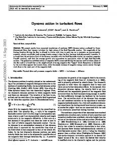
where (also found in the mass and momentum conservation equations) is the velocity with which the CV surface is moving. This equation ensures that the sum of the volume fluxes through all the faces of a CV due to their movement is equal to the rate of change of the volume. The solution domain is first subdivided into a finite number of non-overlapping control volumes, which can basically be of any shape and have an arbitrary number of faces, cf. Figure 2.1 ; for reasons of accuracy, hexahedral CVs are used whenever possible. The CVs can be locally refined by subdividing an existing CV into several smaller ones. In this case the non-refined neighbour CVs – although geometrically still of hexahedral shape – have to be treated as polyhedra, since some of their faces are then replaced by several smaller faces common to the non-refined CV and the newly created smaller CVs. Also, grid blocks of different fineness and topology can be “glued” together and the grids do not have to match at the interface, cf. Fig. 2.2. The numerical grid is therefore unstructured; the number of neighbours can vary from CV to CV and has no upper limit.

N1

n

N6

Nj

n

N2

Sj

C N5

j

N3

C

N4

∆V n

Figure 2.1: A typical control volume and the notation used.

Figure 2.2: An example of a two-dimensional grid with local refinement and a non-matching block interface, showing one quadrilateral CV with six neighbours, N to N .

In order to solve the conservation equations, a Finite-Volume Method (FVM) is used to discretise them on each CV. For each CV, one algebraic equation is then obtained; each of

2.2. OUTLINE OF THE RANSE SOLVER

13

these equations involves the unknown from the CV-centre and from all neighbouring CVs with which the current CV has common faces. Since the equations are non-linear, they have to be linearised in order to be solved by an iterative solution method. The equations are also coupled but are solved in a segregated manner, i.e. for each variable in turn, whereby other variables are treated as known by using the best update available from a previous iteration. In the course of obtaining an algebraic equation for each CV, three levels of approximation are applied:

The integrals over surface, volume, and time are evaluated using midpoint-rule approximations, which use the value of the integrand at the centre of the integration domain. Since the variable values are calculated at CV centres only, values at cell-face centres required for the evaluation of integrals have to be obtained by interpolation; here, linear interpolation is used, except on very coarse grids, where linear interpolation is blended with an upwind-biased approximation. In order to evaluate stress terms (forces) at CV-faces, numerical differentiation is needed to compute derivatives of the Cartesian velocity components with respect to Cartesian coordinates. This is done using either Gauss method or polynomial fitting and central differences, cf. Muzaferija and Perić (1998). The time derivative at the current time level is computed by differentiating a parabola fit through values at the current and two previous time levels; the time integration interval is centred around the current time level (a fully implicit scheme).

All of the above mentioned approximations are nominally of second order. The deferredcorrection approach is used to reduce the implicit part of the discretised equations to the nearest neighbours only; the difference between the simplified and the full approximations is included on the right-hand side of the algebraic equations. This makes the matrix of the algebraic equation system positive definite with diagonal dominance which allows the use of simpler iterative solvers; here, conjugate-gradient type solvers are used (ICCG for symmetric and Bi-CGSTAB, Van den Vorst (1992), for non-symmetric matrices). The mass conservation equation is transformed into a pressure-correction equation following the well-known SIMPLE-algorithm for colocated arrangements of variables, Caretto et al. (1972). In the case of turbulent flows, the standard -& model with wall functions is used. The additional transport equations introduced by the model for the turbulent kinetic energy and its dissipation rate & have a similar form to that of the momentum equations and can be discretised and solved using the same principles. With and & the eddy viscosity ' can be determined. Computation of three-dimensional flows with free surfaces – specially when they are unsteady, as is the case of freely-floating bodies – requires a lot of both memory and computing time. It is therefore essential to be able to perform such simulations on parallel computers. The computer code COMET is parallelised by domain decomposition in both space and time and can use either PVM or MPI message-passing libraries for communication between the processors. Both clusters of workstations and massive parallel computers can be used – as long as they support PVM or MPI standards. Details on parallelisation of the present method can be found in Schreck and Perić (1993) or Seidl et al. (1998).


14

2.2.2 Free-Surface Method In the following, the volume-fraction method used to compute the deformation of the free surface will be outlined. In this method, the solution domain covers both the water and air region around the hull; both fluids are considered as an effective fluid with variable properties, which are determined at any spatial location according to the volume fraction of one constituent fluid (e.g. water). The volume fraction is obtained by solving the corresponding conservation equation, which reads:

!

#

1

(2.5)

The discretisation of the volume-fraction equation requires special attention. Higherorder schemes violate the boundedness requirement, which requires that ; on the other hand, numerical diffusion of low-order schemes must be avoided in order to retain the interface between the two fluids as sharp as possible. Here, the high-resolution interface-capturing scheme (HRIC) is used, which computes the cell-face value of as a blend of upwind and downwind interpolation; see Muzaferija and Peri c´ (1998) for a detailed description. The choice of the blending factor depends on the local distribution of the volume fraction, relative position of the free surface to the cell face, and the local value of the Courant number,

# ! (2.6) is the area of the CV-face , # is the volume of the cell centred around node C,

where and ! is the time step. The Courant number indicates how much of one fluid is available in the donor cell and the scheme is tuned in such a way that no more fluid can drain out of one CV within one time step than was available in it. Another important factor is the orientation of the interface relative to the CV-face. The normal to the interface – which is assumed to lie where the volume fraction has the value 1 – is obtained by computing the gradient of ; it is equal to zero everywhere except in the interface region. Finally, the cell-face value of is computed as:

2 (2.7) where 2 is a non-linear function of the profile of , Courant number, and the orientation of the interface, and C and N denote the nodes on either side of the CV-face ; for more details 2

see Muzaferija and Perić (1998). With this approach, the interface is usually smeared across two to three cells. The fluid properties are computed as:

* * * ' ' '

(2.8)

where subscripts 1 and 2 denote the two fluids (e.g. water and air). If one CV is partially filled with one and partially with the other fluid, it is assumed that both fluids have the same velocity and pressure. The free surface does not represent a boundary and no boundary conditions need to be prescribed at it. If surface tension is significant at the free surface, this can also be taken into account by transforming the resulting surface-tension force into a body force, Brackbill et al. (1992).

2.3. COUPLING FLUID FLOW AND RIGID BODY MOTION

15

2.3 Coupling Fluid Flow and Rigid Body Motion The body-fixed, single-grid strategy mentioned in the previous section is used for both computing the ship’s running attitude and simulating the motion of freely-floating ships. The equations of motion of the rigid body are implemented into the framework of the flow solver package COMET as a user-programmed module, which is linked and run simultaneously with the flow solver. The rigid body module can thus operate and update all flow variables, boundary conditions, and parameters of the numerical method needed to properly couple the fluid flow with the rigid body motions. In this section, the frames of reference used to express the fluid flow and rigid body equations are defined first. Following this, the rigid body motion equations and their integration in time are introduced. The calculation of forces and moments acting on the body, and some peculiarities inherent in this approach, such as the definition of the rotations of the body and the new required boundary conditions on the body and outer flow-boundaries, are then addressed. Finally, an overview of the whole strategy is given.

2.3.1 Frames of Reference Two orthogonal right-handed Cartesian coordinate systems are used: 1. A non-rotating, non-accelerating frame of reference which moves forward with the mean ship speed. It will be denoted in the following by (- ), see Figure 2.3. This frame of reference is a Newtonian reference system in which the equations of linear and angular momentum are valid. The undisturbed free-surface plane always remains parallel to the plane. The -axis points upwards. The position and orientation of the body at any point in time is described with respect to this reference system (RS). The unit vectors . defining this RS are denoted by , and 2. A body-fixed frame of reference with origin at the centre of mass of the body, denoted by ( ). The unit vectors defining this RS are , and . The computational grid always remains attached to this RS as it moves. Following the common practice in ship flow calculations, the -axis is directed in the main flow direction, i.e. from bow to stern, the -axis is taken positive to starboard and the -axis is positive upwards. Thus, we depart from the common practice for sea-keeping and manoeuvring problems where the -axis is positive downwards and the -axis points forwards. Z

z

G

x

Y

O

X

Y

X

y O

G

x

Figure 2.3: Frames of reference.


16

2.3.2 Equations of Motion of the Rigid Body The equations describing the fluid flow, i.e. the RANS equations, are expressed in terms of the coordinates in the Newtonian RS. Thus, the unknowns of the flow solver – the velocities and pressure – and the geometrical quantities are expressed in this RS, so that components of the forces and moments acting on the body are calculated directly in the Newtonian RS. The motion of the rigid body in the 6-DOF are determined by integrating the equations of variation of linear and angular momentum. The equation of variation of linear momentum in the form referred to the centre of gravity is:

(2.9)

the absolute linear acceleration of (i.e. in Newtonian RS), where is the body mass, and is the total force acting on the body expressed in the Newtonian RS. The contributions to the total force are: $ (2.10)

where is the total fluid force determined by integrating the pressure field and viscous stresses, obtained from the Navier-Stokes solver, discretised over the body as:

+

(2.11)

where the subscript stands for each CV face defining the body surface, is the pressure, the normal vector to each CV face (components in Newtonian RS), + the tangential viscous wall shear stress acting on each CV face (components in Newtonian RS), and the CV face area. includes the static and dynamic components for the water and air flow. When the air contribution is negligible, only the hydrostatic and hydrodynamic components are taken is the body weight force, i.e. $ , where is the acceleration of gravity into account. $ acting in the negative -direction. can be any external force acting on the body which one wants to introduce to simulate for instance propeller and rudder forces, the towing force, sail forces, etc. In the 3-D simulations of this work (resistance tests), only the towing force was considered. A component of the towing force is zero if the model is free to move in that direction, or is equal to the hydrodynamic flow force (and in the opposite direction) if the motion is constrained in that direction. For instance, in a resistance test in the model-free condition the vertical component of the towing force is zero, and the components in and directions are opposite to the flow force in these directions. The towing force attachment has to be known. point The equation of variation of angular momentum in the form referred to the centre of gravity can be written as:

" " " "

(2.12)

and are the absolute angular acceleration and angular velocity (i.e. in Newtonian where is the total moment with respect to expressed in the Newtonian RS), respectively, and


17

RS. is the tensor of inertia of the body about the ( ) axes (constant with respect to the body-fixed RS), i.e.:

(2.13)

where is the roll moment of inertia of the ship about the axis calculated as:

3

(2.14)

and analogous for the pitch and yaw moments of inertia ( stands for the whole body mass). , and are the product of inertia (note that , , ), i.e.:

3 1

(2.15)

" in Eq. 2.12 is the transformation matrix from the body-fixed into the Newtonian RS. The columns of " are the unit vectors attached to the body-fixed RS, i.e. , and . The absolute time derivative of the unit vectors, which will be used to find the new orientation of the body, can be obtained as follows:

1

(2.16)

The contributions to the total moment acting on , expressed in terms of the Newtonian RS are: (2.17)

is the total fluid flow moment, discretised as: where

+

(2.18)

are the position vectors of the CV face centres expressed in the Newtonian RS where for all faces defining the body. The towing force was again considered in the 3-D simulations as an external force creating a moment. 2.3.3 Integration of the Body Motion Equations The body motions are described in each time instant by the position of its centre of gravity and the body orientation given by " . For ship motions, the displacements of the centre of mass in two successive time instants are defined in this work in terms of the Newtonian RS as: Surge: Sway: Heave (sinkage):

= ·½

= ·½

= ·½

(translation along ) , (translation along ) , ), (translation along


18

where the superscript ! stands for the actual time instant and ! for the previous time instant, for which the fluid field is known. The new position of in each time step is found by integrating in time the equation of variation of linear momentum, Eq. (2.9). After the first integration the velocity of for the new time instant can be determined as:

! (2.19) ! is the size of the time step in seconds and is a general expression for the force ·½

where acting on the body used for the time integration (mean value over the integration interval). After a second integration the position of for the new time instant can be determined as:

·½

!

(2.20)

is a general expression for the body velocity used for the time integration. where

are approximated, different discretisation methods can be Depending on how and constructed. In this work, different methods were tested. One method was the first order explicit Euler method, for which

1

(2.21)

Another one was a second order explicit method which is obtained with

1

½

1

½ 1

(2.22)

Finally, a first order explicit method in the form

1

½

1 ·½

(2.23)

has shown to be very stable and was preferentially used. This proposed integration method is a mixture of a trapezoid rule using the known forces in the last two time instants to obtain the new velocity and a Crank-Nicolson method for the integration of the velocity to obtain the position of the body. The convergence behaviour of the three methods described above was compared by numerically integrating a harmonic function describing a periodic oscillation (in one DOF) in the form: 5! 6 4 (2.24) with the following coefficients and initial conditions: 1 ; 4 1 ; 5 1 ; 6 ;

1 ;

1. The motion resulting from this function could be one encountered in ship hydrodynamics. The function was integrated over one period systematically varying the time step ! to assess the convergence behaviour of the three methods. Figure 2.4 shows the motion ( ) as a function of time for the second order explicit method. The initial error for the largest time step (! 1 s) is not very large and it is reduced by a factor of four after each halving of the time step. For the first order Euler method, Figure 2.5, the initial error is a bit larger and reduces by a factor of two. Exactly the same behaviour as the Euler method


19

shows the proposed new method, Figure 2.6. For the smallest time step (! 1 s) the first order methods converge quite close to the best result of the second order method, see Figure 2.7. Since the other explicit methods except for the proposed new one behave very unstable in the case of large flow induced accelerations, and since the time steps needed for computing the deformation of the free surface have to be chosen very small anyway, it was considered that the proposed method was a good choice for the small time steps used in the simulations. As we will see in one example of the application of the method (time-accurate simulation of a drop test, Section 5.2), the proposed discretisation delivered acceptable simulated motions.

0.020

0.020

X [m]

X [m]

0.010

0.010

0.000

0.000 ∆t=0.1 s

∆t=0.1 s ∆t=0.05 s ∆t=0.025 s ∆t=0.0125 s

-0.010

-0.020

-0.020 0

1

∆t=0.05 s ∆t=0.025 s ∆t=0.0125 s

-0.010

2

3

4

5

6

0

7

1

2

time [s]

3 4 time [s]

5

6

Figure 2.4: Second order explicit method

Figure 2.5: First order Euler explicit method

0.020

0.020

X [m]

X [m]

0.010

0.010

0.000

0.000

nd

2

∆t=0.1 s ∆t=0.05 s ∆t=0.025 s ∆t=0.0125 s

-0.010

1

ord. exp. (∆t=0.0125 s)

st

Proposed 1 ord. exp. (∆t=0.0125 s)

-0.010

-0.020

-0.020 0

7

2

3 4 time [s]

5

6

Figure 2.6: Proposed first order explicit method

7

0

1

2

3

4

5

6

7

time [s]

Figure 2.7: Comparison of second order explicit and proposed first order explicit methods for ! 1 s.

The new orientation of the body in each time step is found by integrating the equation of variation of angular momentum, Eq. (2.12). Using the same proposed integration method


20

as described above for the linear motions, and after the first integration the angular velocity ·½ is obtained. Instead of integrating again ·½ to obtain the for the new time instant rotation angles of the body, it was preferred in this work to determine the new orientation of the body in a generalised way by integrating the unit vectors of the body-fixed RS, which are the components of the transformation matrix, Puntigliano (2000). Equation (2.16) only needs to be integrated for two of the three unit vectors, for instance to obtain ·½ :

! 1 ·½ (2.25) and analogous for ·½ . The third unit vector, in this case , is determined for the new time ·½

instant with:

·½ ·½ ·½ 1 (2.26) ·½ ·½ ·½ is ortho-normalised in the usual way.

Following this, the new triad

After integrating the equations of variation of linear and angular momentum once and before proceeding with the second integration, the linear and angular velocities at the new time instant are modified in the following cases and with following purposes: 1. Only when the transient characteristic of the motion is not important (e.g. when marching toward a steady-state solution), the convergence of the motion can be improved by retarding the body velocity with:

·½ ·½ ·½ ·½

(2.27)

where is a factor between and and will be called in the following the Delay Factor. The effects of retarding the velocities with will be analysed in detail in the application examples. 2. The motions are constrained in the directions in which the ship is kept fixed, for instance the surge motion with: ·½ 1 (2.28) In this way, if set to zero for ! , it will remain zero throughout the simulation. Also the timing with which the different DOF are released is handled after obtaining the new velocities. The timing for releasing the DOF is important for instance to accelerate convergence or to analyse the effects of the different DOF on resistance in the case of steadystate flows. To simulate transient body motions, all DOF obviously have to be released at the same time. Moreover, the body velocity should not be retarded. More details about this are to be found in the application examples.

2.3.4 Definition of the Rotation Angles From the generalised body orientation at the new time instant given by " ·½ , one is interested in obtaining the angles of rotation of the body for two purposes: 1. To determine the variation of the angles with respect to the last time step for rotating the body from the last into the new position; 2. To determine the absolute angles with respect to the Newtonian RS for monitoring the results of the rotation. The calculation of the angles of rotation demands


21

special care. The order of the rotation has to be defined to be unequivocal. There is more than only one possible definition for the order of rotation, but the following seems to be the most appropriate one for sea-keeping and manoeuvring problems as well as for the ship’s running attitude.

Figure 2.8: Definition of the rotation angles Æ( Æ, Æ) . First, the small rotations Æ) , Æ, and Æ7 for two successive time instants will be defined. Starting from the old body orientation and after was displaced to the new position ( ·½ ), the three rotations are executed in the following order, (see also Figure 2.8): 1. The first rotation Æ) is around the vertical axis in the body-fixed RS ( ), i.e. around . The RS has changed now to ( ·½ ), where and are the normalised unit vectors of the projection of ·½ and ·½ onto the plane, see Figure 2.8. 2. The second rotation Æ, is around the new transverse axis, i.e. around . The RS has changed now to ( ·½ ·½ ). 3. The last rotation Æ( is around the new longitudinal axis, i.e. around ·½ . The RS has finally become ( ·½ ·½ ·½ ·½ ).


22

The equations prescribing the rotations as defined above are:

·½ ·½

·½ ·½

(2.29)

(2.30)

Æ) ·½ Æ, ·½ Æ( ·½

(2.31)

·½

(2.32)

·½ ·½ 1

(2.33)

The absolute rotations with respect to the Newtonian RS are: Yaw (drift) angle: Pitch (trim) angle: Roll (heel) angle:

) ·½ = ) ·½ , ·½ = , ·½ ( ·½ = ( ·½

), (rotation around (rotation around ) , (rotation around ·½ ) .

and , They are calculated using the same equations above but replacing and with respectively. 2.3.5 Boundary Conditions At this stage only the peculiarities in the boundary conditions due to the motion of the body (and thus the grid) will be addressed. The standard boundary conditions will be addressed in Section 3.3. The no-slip boundary condition at the body wall implies that the velocity of any point on the hull surface and the fluid velocity must be identical. Since the body is translating and rotating with respect to the main direction of the flow, the motion velocities have to be imposed at each CV face defining the body as boundary condition. For this purpose the equation of the state of velocities is used, which expresses the velocity of any point of the rigid body as a function of the velocity of a reference point – in this case of – and the angular velocity of the body: 1

(2.34)

Since the flow solver needs all variables expressed in terms of the Newtonian RS, Eq. (2.34) is also expressed in terms of the Newtonian RS. To set the boundary conditions at the external boundaries when using the approach of a single grid following the body motions becomes a critical issue. If a grid line at the external boundaries of the computational domain coincides with the position of the undisturbed free-surface plane, to set the boundary conditions for the volume fraction equation (and depending on this the other variables) is a trivial task. For all CV faces which lie completely above the undisturbed free-surface plane, the volume fraction is set equal to one, and for


23

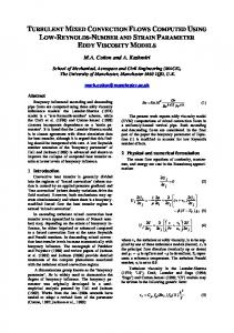
those underneath, equal to zero. This would most likely be the configuration found in the outer space-fixed grid, if the two-grid system were used. If the grid lines in the region of the free surface are aligned with the undisturbed free-surface plane but shifted by some amount so that no one coincides with it, the volume fraction can then also be easily calculated as a function of the distance of the CV face centre to the undisturbed-free surface. A problem arises when the grid lines are not even parallel to the undisturbed free-surface plane and when their relative position to it is changing in every time step. This is the case in the single grid approach. In all CV faces at the boundaries which are crossed by the undisturbed freesurface plane an interpolated value (between and ) for the volume fraction have to be set. In this way, the CVs at the external boundaries have no restriction in size and the transition from water to air at the free surface is smooth. The volume fraction distribution is updated every time step as the grid moves with respect to the undisturbed free-surface plane, which is fixed in space. An accurate interpolation of the volume fraction is performed at every time step by means of a procedure which calculates the truncated areas (and volumes) of arbitrary shaped CVs. The interpolation procedure has been implemented by Albina (2000), and was extensively tested in this work. It is not only used to set the boundary conditions at every time step but also to accurately initialise the volume fraction field in the whole computational domain in order to accelerate the convergence at the beginning of the computation. Figure 2.9 shows an example of such an interpolated volume fraction distribution. It represents a keel boat (this example will be introduced later in this work) which is inclined Æ to one side. The blue coloured CVs represent the water, the white CVs the air. The thick black line at the free surface has been plotted interpolating the actual values of the CVs.

Figure 2.9: Example of an accurate volume fraction interpolation for boundary and initial conditions.


24

2.3.6 Coupling Algorithm The coupling of the body motion equations with the flow solver in a time-marching procedure is organised as follows: 1. Input data at !

! :

¼ . Initial position of the centre of gravity of the body Initial orientation of the body as ( ¼ , ¼ ) ¼ .

¼ and angular velocity ¼ of the body. Initial linear velocity

DOFs to be considered, the timing for releasing them and the delay factors. Position and line of action of the external forces.

Body mass and tensor of inertia of the body . Initial position of the undisturbed free-surface plane with respect to the body-fixed RS. Ship speed (speed of the Newtonian RS) and other flow parameters.

2. Position ship in its initial attitude. For this purpose the whole grid is rotated and translated with respect to the Newtonian RS. Calculation of the initial transformation matrix " ¼ . 3. Initialise flow field; velocity and pressure field in water and air, volume fraction for water and air according to position of the undisturbed free-surface plane, turbulence parameters, etc. 4. Set boundary conditions at the body wall (no-slip condition) according to Eq. (2.34). 5. Set interpolated boundary conditions at external boundaries (inlet, outlet, symmetry, etc). 6. Calculate forces and moments in the Newtonian RS for the last position from the pressure and velocity field from the flow solver (from the initialisation for ! ! ). 7. Output forces and moments, velocities, displacements and angles, coefficients, etc, for monitoring the convergence and time histories. 8. Integrate equation of linear and angular momentum of the body to obtain new position ·½ and orientation " ·½ of the body, Eq. (2.19) to (2.26). 9. Move grid with body attached to it into the new position; first the linear translations with respect to the Newtonian RS and then the rotations around the axes of the body-fixed RS. 10. Compute fluid flow around the body for the new position with the RANSE flow solver. 11. Set old values equal to new ones (position, orientation, linear and angular velocities of the body), and update the external forces. 12. Increment time step ! ! !, and proceed at point 4 with the next time step.

Chapter 3 Steady Free-Surface Flows Around Ships 3.1 Introduction This chapter presents the first task of this thesis, which is to assess the achievable accuracy of numerical resistance predictions using Navier-Stokes solvers like the one used in this case, the program-package COMET. Researchers around the world increasingly recognise the need for predicting all components of ship resistance by means of a single code, taking into account the coupling between the components. In this context, the validation of the numerical method and the uncertainty analysis of the results are very important. For this purpose, calculations of the turbulent free-surface flow around ships advancing steadily in calm water are presented in the following. Although some computations were performed for the full scale ship, the calculations presented in this chapter are for the model scale, for which experimental data from towing tanks were available. In this way, some issues that have a significant influence on the achievable accuracy of the numerical results could be addressed. Special attention is paid to the dependence of the friction resistance component on grid quality and resolution at no-slip walls, and also to the dependence of the pressure resistance component on the type of discretisation scheme used for the momentum equations. Furthermore, a strategy for achieving good convergence with little computational effort is addressed, and a novel type of extrapolation to obtain near grid-independent solutions for pressure resistance without computing on extremely fine grids is proposed. The analysis presented in this chapter reproduces the work already published in Azcueta (2000). It represents the basic knowledge and experience which was needed at a later stage to improve the resistance prediction by including the change in the ship’s running attitude. All issues mentioned in this chapter, such as the boundary and initial conditions, the type of time integration, the type of spacial discretisation, turbulence modelling, etc. are also valid for the simulations introduced in the following chapters (ship’s running attitude and freely-floating body motions) unless at that point otherwise stated. In the following, the grid generation procedure is briefly described and the boundary and initial conditions are addressed. The test cases used in this analysis as well as some general aspects and the first results and validations are then presented. Finally, the accuracy of the resistance prediction is analysed in detail.

25

26

CHAPTER 3. STEADY FREE-SURFACE FLOWS AROUND SHIPS

3.2 Grid Generation Grid resolution and grid quality play a crucial role for the accuracy of viscous flow calculations. In this work, grids made of hexahedral CVs which deliver the best accuracy were used in most cases unless otherwise noted. When the ship geometry is simple, single-block structured grids are preferred. Sometimes a multi-block grid is necessary, where the mesh points at both sides of the interface are made to match whenever possible. Non-matching interfaces between blocks have not been used so far in the applications shown here, but it can be a possibility well worth considering in some cases. Local grid refinement is a very good way to improve resolution and grid quality in those regions where large changes in gradients of computed variables are found. This strategy has often been applied. For the application examples to be introduced in this thesis, the numerical meshes were generated in the following ways:

analytically, when the ship geometry was very simple or mathematically describable, as in the case of the Wigley model and the flat-plates. The latter were used to check the performance of the turbulence model. To generate these meshes, Fortran routines were programmed and customised for each case. with the grid generation utility of the program-package COMET, also for relatively simple geometries like for the semi-circular bow ship and for the prismatic wedge, which will be introduced in Sections 4.3 and 5.2, breaking waves and drop tests, respectively. using an elliptical grid generator developed by Cura Hochbaum (1993), when the ship geometry was complicated as it is the case of conventional ships with bulbous bow. As input data for this grid generator, the distribution of all points at the boundaries of the computational domain have to be carefully selected, defining in this way the mesh topology. Crucial in this sense is the panelisation of the hull geometry, which was done using a program for describing and interpolating ship hull surfaces, S o¨ ding (1992). The input data and ship lines interpolation programs have to be customised for each new case. This approach was used to generate the grids for the Series 60 hull, the hydrofoil with laminarflow profile, the container ship with bulbous bow, and the sailing yacht. Details of those grids will be given in the respective sections. The elliptical grid generator used ensures that the grid lines are nearly orthogonal to each other and allows a much better control of the spacing between grid layers, specially at the ship wall. Grid line orthogonality and constant spacing are of vital importance to obtain the high quality grids needed in calculations of viscous flows around ships.

In all cases, the grid resolution is chosen high near the ship wall to resolve the boundary layer better, as well as in the proximity of the free surface to capture the it’s distortion as well as possible. The grid lines expand smoothly in all directions away from the ship and the free surface. Furthermore, the CVs are clustered at bow and stern to capture the highly varying gradients better in those regions. If the ship and the flow are symmetric, i.e. in most ships advancing straight ahead, only one half of the hull is considered. The computational domain usually extends, depending on the Froude number, 1 ahead of the ship, 1 to 1 to the side and in the wake, and 1 below the design waterline. Furthermore, the domain is extended with an additional block above the maximum wave height expected to ensure that the air flow between the waves and the upper

3.3. BOUNDARY AND INITIAL CONDITIONS

27

boundary has got enough room to flow and does not artificially accelerate due to a blockage effect. This would increase the bow-wave height to some extent and thus introduce additional errors in the solution.

3.3 Boundary and Initial Conditions For incompressible flows, as in the case of the flow around ships, the inlet boundary condition can be specified at that portion of the boundary where the velocity distribution is known, usually in front of the ship. Sometimes, other flow boundaries, i.e. boundaries that do not represent a physical wall but an unphysical cut through the fluid domain, such as the side, bottom and top of the ”numerical tank”, have also to be specified as an inlet. This is the case when the flow boundaries are not parallel to the undisturbed flow, either when the grid has been generated like this or in the simulation of freely-floating body motions, since the computational domain is constantly moving fixed to the body and relative to the flow. Otherwise, for steady flow calculations in the model-fixed condition when the flow boundaries (at the side, top and bottom) are parallel to the undisturbed flow, they can be specified as slip walls. For computations with a free surface, the water velocity is set (at the inlet) equal to the ship speed being investigated, but in the opposite direction. The air velocity is set equal to the water velocity, if a no-wind condition is assumed, or otherwise in any other direction and speed. Since the computed flows are turbulent, the turbulence parameters have to be specified at the inlet as well. It is assumed that the free-stream turbulence intensity is about and that the turbulent viscosity is of the same order as the molecular viscosity. The distribution of water and air is specified at the inlet relative to the position of the undisturbed free-surface plane by means of the volume fraction of one fluid into the other, which determines the densities of both fluids, as was explained in Section 2.3.5. The outlet boundary condition is usually specified where the flow leaves the computational domain and where it can be assumed that the zero gradient condition applies. In free-surface computations the known hydrostatic pressure (according to the relative position of the undisturbed free-surface plane) has to be specified at the outlet as well. At the body wall or ship hull, the non-slip condition is specified. If the body is moving, the non-slip condition is warranted using the equation of the state of velocities as explained in Section 2.3.5. Since the standard –& turbulence model is used to simulate the turbulence effects on the mean flow, wall functions are used to prescribe the velocity distribution in the boundary layer. No special treatment of the turbulence has been incorporated for the free surface yet. To start the simulation, the inlet boundary conditions ( , , and 8) at full ship speed are also imposed over the entire computational field without accelerating the flow from rest. That means that at ! the flow at the hull wall is not aligned with the wall and large velocity gradients appear after the initialisation. The numerical method was shown to be robust enough to cope with this kind of shock, and faster convergence towards steady-state conditions is attained in this way. A problem usually found in these types of calculations (specially in two dimensions), is that the pressure resistance oscillates due to waves reflected at the non-physical side boundaries. A way to avoid this is to use a numerical damping or beach at the side boundaries. In

28


the flow computations of this work, the radiating waves dissipate sufficiently due to numerical diffusion in the larger CVs near the side boundaries. For this purpose, the grids were generated using large expansion factors (around 1 or 1) in order to concentrate most CVs near to the ship and get larger CVs further outside. In this way, the wave pattern is best captured and wave reflection from the boundaries is minimised without using artificial damping. An alternative preferred by other authors is to distribute the CVs more regularly over the entire computational domain, and to use artificial damping, Schumann (1999).

3.4 Test Cases In this section the test cases used to investigate the accuracy of the numerical resistance prediction will be presented. The test cases were the Wigley hull, the Series 60 hull, a modern container ship, and a hydrofoil with laminar-flow profile. The flow around the Wigley and the Series 60 hulls was extensively investigated and validated with the available experimental data. Some results for the Wigley hull and the Series 60 hull will be shown in the next two sections and a more detailed discussion of the main factors affecting these results will be addressed in the subsequent sections.

3.4.1 Wigley Hull Although the Wigley hull as a test case has to some extent become obsolete for comparing the performance of numerical methods, it is sometimes still used because of its simple geometrical form, which simplifies grid generation, and also due to the large amount of experimental and computational data available for validation. In this thesis, it is only used to ratify the phenomena which are being investigated. The Reynolds number 1 and the Froude number 1 (both based on hull length) in the computations correspond to the model tests ( model) performed at the Ship Research Institute (SRI) in Japan. Three grids were used with , and CVs, respectively. Table 3.1 lists for each grid the number of CVs along the hull ( ), normal to the hull ( ) and in the vertical direction ( ). Also listed in the table are the spacing between grid lines in -direction ( ) at bow and stern (larger at ) and in -direction ( ) in the range of the free surface. In -direction, the spacing varies for the three grids from 1 at the bow to 1 at the stern, in an attempt to keep a constant dimensionless wall distance . Finally, Table 3.1 also lists the computer used and the CPU time needed to perform time steps. Within this time the ship moves forward approximately . Only one outer iteration per time step was performed (pseudo-steady time integration), see Section 3.6. Table 3.2 compares the predicted resistance coefficients for the three grids with the measured total resistance. The experimental data was taken from the SRI, Anon. (1983). Both the calculated and experimental values are in this case for the model-fixed condition. The value in the experiment was determined from the ITTC57 correlation line, i.e. 1 . The residual resistance coefficient is calculated as the measured total resistance coefficient minus . The friction (pressure) resistance coefficient from the calculations is obtained as 1 * , where

3.4. TEST CASES

29

Table 3.1: Wigley hull: CVs and grid spacing, computer used and CPU time. Grid coarse medium

CVs

fine

1

1

1

1

1

1

computer

CPU [h]

pentium 166 SGI 900, 1 proc. pentium 166 SGI 900, 8 proc. SGI 900, proc.

1

1

is the computed total friction (pressure) force in -direction (ship-fixed reference system), * the fluid density, the model speed and the wetted surface of the model at rest. The computed values depend on the size of the time step and on the blending factor for the discretisation of convective fluxes in the momentum equations. For the results shown in Table 3.2, they were set at ! 1 s and central differencing. In Sections 3.6 and 3.8, respectively, a description of these parameters and a more detailed discussion of the achievable accuracy will be given. Table 3.2: Comparison of the resistance coefficients for the Wigley hull. Calculations on three grids and experiments from SRI, Anon. (1983). Grid experiment coarse medium fine

1 1 1 1

( ) 1 1 1 1

1 1 1 1

1 1 1

Figure 3.1 shows the wave height contours (wave pattern) once the converged steadystate solution was reached, as computed on the three grids. The difference in wave pattern between the three grids is quite noticeable. In Figure 3.2, the free-surface elevation along the hull surface, as computed using the three grids, is compared with experimental data. The agreement is quite satisfactory for all grids, although the wave pattern on the coarsest grid differs substantially from that on the medium and fine grids.


30

0 mm

0 mm

0 mm

Figure 3.1: Computed wave pattern around the Wigley hull at bottom: coarse, medium and fine grid. Interval between lines: 1 .

1

. From top to

zeta/L 0.014

coarse grid

0.012

medium grid

0.01

fine grid

0.008

UT-Experiment

0.006 0.004 0.002 0 -0.002 -0.004 -0.006

0

0.2

0.4

0.6

0.8

1

x/L

Figure 3.2: Predicted and measured free-surface elevation along the Wigley hull at

1 (present computations on three grids; experiments from the University of Tokyo).

3.4. TEST CASES

31

3.4.2 Series 60 Hull The Series 60 hull with a block coefficient 1 was selected as another test case, as both experimental data and results from many other numerical computations are available for it, since it was used as a test case at the CFD Workshop in Tokyo 1994. For the present study, the flow was computed at a Reynolds number (model scale) and a Froude number 1 . Results are compared with experimental data from the University of IOWA, Toda et al. (1992). Computations were carried out on three numerical grids, which were systematically refined. The coarsest one had , the medium one

, and the finest one CVs. Table 3.3 lists for each grid the total number of CVs and the number of CVs in each direction; along the hull ( ), normal to the hull surface () and along the girth of the hull section ( ). The table also lists the mesh resolution at the hull, the minimum spacing between grid lines in -direction at bow and stern ( , larger at ), and in the -direction (, variable from bow to stern) with the corresponding dimensionless wall distance averaged for , and finally the spacing in -direction at the free surface ( ). At the CFD Workshop 1994 in Tokyo, the following recommendation for the minimum CV size in order to correctly capture the transverse and diverging waves was given: 9 1 and 9 1 for 1 , which corresponds to about to CVs per wave length, Mori and Hinatsu (1994). For instance, on the finest grid used in this work, the criterion is satisfied along the hull where the largest CVs at are 1 long. In the wake it is satisfied up to 1 behind the stern. The criterion is only satisfied close to the wall (up to 1 ), because a high resolution is needed to resolve the boundary layer and most CVs are clustered near the wall. Table 3.3: Series 60: CVs and grid spacing. CVs

at hull

min

1 1 1

(bow/stern) 1 1 1 1 1 1

1 1 1

The CPU time needed to compute time steps (only one outer iteration per time step), equal in this case to the time needed for a water particle to travel nearly , was 1 h, 1 h and 1 h for the coarse, medium and fine grids on a SGI 900 parallel computer with one, four and eight processors, respectively. Figure 3.3 shows a comparison of computed and measured wave patterns for the three grids. Both measurement and computations were performed in this case at model-fixed condition. The improvement with grid refinement is only remarkable at a certain distance from the hull. The wave profile along the hull obtained with the coarse grid already shows a good agreement with subsequent finer grids, cf. Figure 3.4. The wave profiles obtained on the medium and fine grids do not change much, indicating that the agreement with measured values will still not be as satisfactory as for the Wigley hull. The computed forces for the Series 60 hull will be presented in detail in Sections 3.8 and 4.2.

32


0 mm

0 mm

0 mm

0 mm

Figure 3.3: Computed and measured wave patterns around the Series 60 hull at 1 . From top to bottom: coarse, medium, and fine grid and experiments.

zeta/L 0.015 coarse grid medium grid fine grid measurement IIHR

0.010

0.005

0

-0.005

-0.010

-0.015 0

0.2

0.4

x/L

0.6

0.8

1

Figure 3.4: Computed and measured wave profiles along the Series 60 hull at 1 . Model-fixed condition.

3.4. TEST CASES

33

3.4.3 Other Test Cases To broaden the series of test cases used to investigate the validity of the proposed extrapolation to grid-independent solutions for pressure resistance, calculations for the model of a container ship and for a 2-D hydrofoil with laminar-flow profile (typically used for yacht keels) were performed. Figure 3.5 shows the surface mesh used to calculate the free-surface flow around the container ship. It has a large bulbous bow and a submerged transom. This case is an example of a modern ship hull shape, which demanded a great effort in order to generate a mesh of good quality. Two meshes with and CVs were used. The model length was m, the Froude number 1 and the Reynolds number 1 . The calculation was performed for the model-fixed condition. For the flow around the 2-D hydrofoil, three systematically refined grids with , , and CVs, respectively, were used. Figure 3.6 shows a close-up view of the medium grid. All radial mesh lines are basically orthogonal to the foil wall. The spacing between grid layers is well controlled, expanding smoothly in all directions away from the foil. Results obtained for this two test cases will be presented in Section 3.8.

Figure 3.5: Surface mesh for the flow around a modern container ship.

Figure 3.6: Elliptical mesh for the flow around a 2-D hydrofoil (medium grid).

34


3.5 Dependence of Friction Resistance on Grid Quality Using the standard –& turbulence model with wall functions is a good choice for computing ship flows including the free surface, as well as for computing the flow at full scale, as lower grid resolution is admissible at the wall, and by this, allowing to concentrate the CVs at the free surface or going for a higher Reynolds number. However, for computations at model scale, this model is affected by a strong dependency of the computed friction resistance coefficient on the distance from the wall to the first CV centre. This fact demands great care and experience in mesh generation. The common belief that the range of validity of wall functions extends up to or even is not correct for computations at the typical Reynolds numbers at model scale. An upper limit of appears more appropriate. In Figure 3.7, computed integral friction resistance coefficients for the Wigley hull are compared to the ITTC value for the same Reynolds number. The computations were performed on seven different grids in which the distance from the wall to the first CV layer (spacing) was systematically varied. The first grid (marked 1 in Figure 3.7) had a constant spacing along the hull and thus a variable of about at , with higher values at the bow and lower ones at the stern due to the decelerating flow. The value of on this grid was about lower than the ITTC. The second and third grids also had a variable of about and , and differed from ITTC by and , respectively. For the fourth grid with a value of about the calculation did not converge. The fifth and sixth grids had a variable spacing and thus an almost constant . To achieve this, the grids were generated using a spacing calculated for each -location as a function of the local Reynolds number. The last grid (marked 7 in Figure 3.7) was similar to the last two, but the spacing to the first CV centre was kept constant in the girth-wise direction as well. In this way, the friction resistance prediction for the case was improved. 0.0034

CF ITTC 0.0033

3

0.0032

7 6 5

0.0031

2

0.0030

CF calc. 0.0029

0.0028

0.0027

1 0.0026 0

50

100

150

200

250

300

350

400

450

Y+

Figure 3.7: Dependence of on computed for the Wigley hull. To investigate the performance of the –& turbulence model in detail for this Reynolds number range, calculations with flat plates of finite length were also performed. The same strong dependence of on was found. For these calculations, the Reynolds number based on the plate length was set at , which corresponds to the Reynolds number

3.5. DEPENDENCE OF FRICTION RESISTANCE ON GRID QUALITY

35

for the small models of the Wigley and Series 60 hulls investigated in this work. The number of CVs used were also of the same order of magnitude as in the ship flow computations ( along and normal to the plate). Two sets of calculations were performed. In the first one, the spacing from the wall to the first CV centre (constant along the plate length) was varied. From there, the rest of the grid lines expanded evenly to the side boundary situated plate lengths away. Thus, the resolution close to the plate also varied. In the second set, the whole grid was kept unchanged but only the first grid line close to the plate was moved to match the different values. Both sets of calculations produced similar results. The differences due to varying the resolution by keeping the same value were minimal, indicating that the discrepancies are due to a model error and not to resolution or discretisation errors. In the following, only the results for the first set of calculations will be shown. The values, averaged at , were approx. , , , and . Figure 3.8 shows the computed integral for these cases, compared to the ITTC value for the same Reynolds number. For the case, the difference from the ITTC value was , while for the last two it was about 1 . Figure 3.9 shows the distribution of the local skin friction coefficient along the plate length for the different values compared with the theoretical line for turbulent flow on a plate given by Schlichting and Gersten (1997). For , the calculated and theoretical lines do not have much in common. Only if the plate were much longer for the given grid spacing in normal direction, and thus for a higher , the calculated line would approach the theoretical one. This means that the boundary layer on that grid could not fully develop as it should. Only for the two finest grids ( and ) the correspondence to the theoretical line is acceptable. Note, however, that the calculated lines run above and below the theoretical one, which indicates that the errors partially cancel each other, resulting in a better integral value for . An additional calculation was performed with the grid, with the front of the plate being locally refined, until was reached. The improvement in this case was only local (in the refined region) with the boundary layer resolution getting worse immediately behind the refined region (line with the sharp corner by 1 in Figure 3.9). In Figures 3.10 and 3.11, mean velocity and turbulence kinetic energy profiles for the plate boundary layer are plotted in dimensionless form. These two figures confirm that, for the case at this Reynolds number, the boundary layer is resolved only with grid points, which is insufficient. In the case, there are at least grid points inside the boundary layer at and at the trailing edge. Both velocity profiles are in good agreement with the log-law line depicted in the figure. A similar, qualitatively incorrect distribution of the computed local skin friction coefficient was also observed for the flow around the Wigley hull on the grid. Those profiles are not shown here due to lack of experimental data available for comparison. As a conclusion, it can be said that varying the spacing to the first CV centre along the ship length to take into account the decrease of boundary layer thickness towards the bow, slightly improves the prediction of friction resistance. With the grid generation procedure used for this calculations of ship flows, taking into account the variation of grid spacing along the hull was a simple task, so that it was implemented for all grids. Another alternative could be to adapt the grid spacing interactively during the computation (re-gridding) in order to keep a constant value or a suitable number of grid points inside the boundary layer. For this purpose, the author suggests to use a value of close to or to assure that the first


36

0.0036

0.008

Cf (Schlichting)

CF ITTC

0.0034

Cf (Y+~25)

0.0032 0.003

Cf (Y+~50)

0.0028

Cf (Y+~25/400)

CF calc. Cf (Y+~100)

0.0026 0.001 Cf (Y+~200)

Cf (Y+~400)

0.0024 0.0022

0

50

100

150

200

250

300

350

400

450

0.0005

Y+

0

0.1

0.2

0.3

0.4

0.5

0.6

0.7

0.8

0.9

1

x/L

Figure 3.8: Dependence of on the turbulent flow along a flat plate.

for

28

Figure 3.9: Distribution of local along the plate for different values compared with theoretical line.

3.5

U+

Y+~25 x=1.0 26 Y+~25 x=0.5

Y+~400 x=1.0 Y+~25 x=1.0

K+ 3

24 2.5

Y+~400 x=1.0 22

2

20 1.5

18 1/0.41*ln(Y+)+5.35

1

16

0.5

14 12

100

1000 Y+

Figure 3.10: Mean velocity profile compared to log-law. grid at trailing edge and grid at trailing edge and at .

0

500

1000 1500 2000 2500 3000 3500 4000 4500 5000 Y+

Figure 3.11: Turbulence kinetic energy profile for and grids at the plate trailing edge.

point is within 1 to 1 of the boundary layer thickness, whichever is smaller. This second alternative would yield better results, because the dimensionless wall distance is much more affected by local form effects (acceleration, deceleration or even separation of flow) than by the normal boundary layer development along a flat plate. It is difficult, however, to implement, and requires more computational effort. Fortunately, the model error introduced by the wall functions decreases in importance for higher Reynolds numbers. Since the ultimate goal is the computation of the flow at full scale, the standard –& turbulence model with wall functions is still a valid option to work with.

3.6. EFFECTS OF TIME STEP ON RESISTANCE

37

3.6 Effects of Time Step on Resistance Another critical issue with respect to the resistance prediction is the choice of the size of the time step ! needed for the time integration procedure. ! has to be chosen within certain limits. If it is too large, the integration procedure used (pseudo-steady) becomes unstable. If it is too small, the Rhie and Chow (1983) correction will not work properly, the pressure and velocity fields can become decoupled and the calculation oscillates and finally diverges. Unfortunately, pressure and friction resistance coefficients depend on the ! used, which means that several runs have to be calculated in order to assess the level of uncertainty by varying !. The fact that the steady-state solution depends on ! stems from the appearance of ! in the effective interpolation formulae for the computation of the cell-face velocities and the volume fractions (Rhie & Chow correction term and the HRIC scheme, respectively). The dependence reduces as the grid is refined, but since in 3-D applications the level of refinement is quite limited, it was important to investigate these effects. Figures 3.12 and 3.13 show the effects of ! on resistance coefficients for the flow computation around the Wigley hull and the Series 60 hull, respectively, on three grids. The computations were started with a large time step (i.e. ! 1 s), and this was progressively halved until no longer converged. For the Wigley case, the variation in for all grids was about , which is very significant. varied by . For the flow around the Series 60 hull, the change of was between and , while varied by about . Figure 3.14 shows and convergence histories with varying ! for the flows around the Wigley hull and the Series 60 hull, respectively, on the medium grid. While for the Wigley hull there is a clear trend on when reducing !, the Series 60 case shows no convergence. For ! 1 s (between and s), becomes smaller than for ! 1 s and ! 1 s. Figures 3.15 and 3.16 show the wave pattern and the wave profiles (the latter compared with experimental data) for the flow computations around the Wigley and the Series 60 hulls on the medium grids, respectively, for four ! values: 1 1 1 1 s. The wave pattern resolution clearly improves as ! is reduced. In the Wigley case, ! was halved two more times (1 1 s), but then the wave pattern and profile did not change any more. In the Series 60 case, reducing ! beyond 1 s made the results behave unstable, as can be seen in the convergence history in Figure 3.14. Why for the Series 60 case does not converge for smaller ! like in the Wigley case is not clear. As stated above, there are two sources for the dependence of the results on !. One is the Rhie & Chow correction term, which limits the minimal size of ! for which the results are free from oscillations. The second and most dominant one is a Courant number correction in the used discretisation scheme for the volume fraction (HRIC). These two !-dependent corrections may interact with each other, and it is difficult to separate their effects. It should be noted that this dependence of on ! is not a consequence of the pseudo-steady time integration. Exactly the same results are obtained if several outer iterations per time step are made.


38 0.00115

0.0033

coarse medium fine

0.0011

coarse medium fine

0.00328 0.00326

0.00105

0.00324 0.00322

Cp

0.001

Cf

0.0032 0.00095

0.00318 0.00316

0.0009 0.00314 0.00085

0.00312 0

0.005

0.01

0.015

0.02

0.025 δt

0.03

0.035

0.04

0.045

0

0.005

0.01

0.015

0.02

0.025 δt

0.03

0.035

0.04

0.045

Figure 3.12: Dependence of the pressure (left) and friction (right) coefficients on ! on three different grids for the Wigley hull.

0.00182

0.00355

0.0018

0.0035

0.00178

0.00345

0.00176

0.0034

0.00174

0.00335 Cp

0.00172

coarse medium fine

0.0033

0.0017

Cf

0.00325

0.00168

0.0032

0.00166

0.00315 coarse medium fine

0.00164 0.00162 0

0.005

0.01

0.015

0.02

0.025 δt

0.03

0.035

0.0031 0.00305 0.04

0.045

0

0.005

0.01

0.015

0.02

0.025 δt

0.03

0.035

0.04

0.045

Figure 3.13: Dependence of the pressure (left) and friction (right) coefficients on ! on three different grids for the Series 60 hull.

Cf

Cf

Cp Cp 0.001

0

20

40

60

80 100 120 elapsed time [s]

140

Figure 3.14: Convergence history of Series 60 hull. Medium grids

160

180

and

0.001 0

50

100 150 elapsed time [s]

for varying !.

200

250

Left: Wigley hull; right:

3.6. EFFECTS OF TIME STEP ON RESISTANCE

zeta/L 0.014 0.010 0.006 0.002 -0.002 -0.006

0.02dT

UT-Experiments

0

0.2

0.4

0.6

0.8

39

zeta/L 0.014 0.010 0.006 0.002 -0.002 -0.006

1

0

0.2

0.4

x/L

zeta/L 0.014 0.010 0.006 0.002 -0.002 -0.006 0.2

0.4

0.6

0.8

1

x/L

0.005dT

UT-Experiments

0

0.01dT

UT-Experiments

0.6

0.8

zeta/L 0.014 0.010 0.006 0.002 -0.002 -0.006 0

1

0.0025dT

UT-Experiments

0.2

0.4

0.6

0.8

1

x/L

x/L

Figure 3.15: Wave pattern and profile (latter compared with measurements) for the flow around the Wigley hull using four different ! (medium grid: CVs).

zeta/L 0.015

0.02dT

Experiments IIHR

0.01

zeta/L 0.015

0.01dT

Experiments IIHR

0.01

0.005

0.005

0

0

-0.005

-0.005

-0.01

-0.01

-0.015

-0.015 0

0.2

0.4

0.6

0.8

1

0

0.2

0.4

x/L

zeta/L 0.015

0.005dT

Experiments IIHR

0.01

0.6

0.8

1

x/L

zeta/L 0.015

0.0025dT

Experiments IIHR

0.01 0.005

0.005 0

0

-0.005

-0.005

-0.01

-0.01 -0.015

-0.015 0

0.2

0.4

0.6 x/L

0.8

1

0

0.2

0.4

0.6

0.8

1

x/L

Figure 3.16: Wave pattern and profile (latter compared with measurements) for the flow around the Series 60 hull using four different ! (medium grid:

CVs).


40

3.7 Strategy for Best Convergence Trying to obtain a steady-state solution for a free-surface flow using a time-marching method needed for unsteady flows seems a priori not to be the best possible solution. The problem which made direct, stationary solutions impossible so far resides in the unknown free-surface position. This is usually overcome by considering the flow transient and by integrating in time until a steady-state solution is reached. Thus, the computational effort is of at least one order of magnitude larger compared to a steady flow without free surface. However, all calculations with free surface published so far are embedded in time integration procedures, although there is consensus among researchers on the need of getting rid of the time integration. Nevertheless, in order to achieve the best possible convergence towards the steady-state solution for free-surface flows using this numerical method, the following strategy was followed:

computations were started with the full flow speed, i.e. without accelerating the flow from rest, or alternatively the solution obtained on the next coarser grid was used as initial condition.

only one outer iteration per time step was performed throughout the computation, ! (unique for all CVs) was varied from the largest possible at the beginning to the suffi

ciently smallest at the end.

It was generally observed in all these computations, that with only one outer iteration per time step (what we call pseudo-steady time integration), the computations converged faster to the steady-state solution, than by doing more than one iteration per time step, but fewer time steps. Furthermore, it is not necessary to satisfy a convergence criterion for outer iterations (of three to four orders of magnitude), because this does not improve the results any further once the steady-state solution has been reached. As mentioned above, ! has an influence on the results. The best results are obtained with the smallest possible !, for which convergence is still achieved and the variable fields do not oscillate. For this solution, one can also observe a wave pattern that best approximates the measured one, cf. Figures 3.15 and 3.16. The question is then how to reach this solution with a minimal computational effort. Because the pressure coefficient oscillates strongly (due to the reflection of the radiating waves), it is convenient to try to reduce the oscillations as fast as possible in the first instance. For this purpose it is better to start the computation with the largest possible time step, so that more time units (time that a particle takes to travel ) are calculated with fewer time steps. In doing so, the amplitude of the oscillations decreases faster than by calculating fewer time units with a smaller ! in the same amount of time steps. Once the amplitude of the oscillation is substantially reduced, one can halve ! and continue the computation, and then repeat this procedure as many times as required to obtain the best possible results. This procedure can be set before the start of the calculation and run automatically. Results for each ! can be saved for comparison.

3.8. INFLUENCE OF DISCRETISATION SCHEME ON PRESSURE RESISTANCE 41

3.8 Influence of Discretisation Scheme on Pressure Resistance To calculate convective and diffusive fluxes, variable values and their gradients are needed at the CV faces. They have to be interpolated from their values at CV centres. There are many possibilities to do this. One is to use the first order upwind differencing scheme (UDS), which is numerically diffusive and should therefore be avoided. A second one is the widely used second order central differencing scheme (CDS), which offers a good compromise between accuracy, simplicity and efficiency. However, it may produce oscillatory solutions, so that it has to be blended with some amount of first order UDS. This blending with UDS introduces a numerical error, which in the case of ship flows can be quite significant, depending on the amount of UDS used. Large variations in the pressure resistance are the consequence, while the effects on the friction resistance are comparatively small. In order to assess the variation of the pressure resistance coefficient for the different discretisation schemes resulting from blending UDS with CDS, four different flow cases were systematically studied by varying the mixing ratio of UDS-CDS. The cases chosen were the Wigley hull, the Series 60 hull and the modern container ship using the grids described earlier (free-surface flows), as well as a two-dimensional flow around a foil section deeply submerged and at zero incidence (no free surface). For each flow case and on the three grids (two grids for the container ship), calculations were performed using blending factors varying in 1 steps from pure UDS to the maximum possible amount of CDS, typically to depending on the flow case, grid quality and fineness. In each case, the calculations were carried out for as many time steps as was necessary to allow a good average for , after the small oscillations produced by changing the discretisation had vanished. A huge computational effort was therefore necessary to complete the set of computations for the finer grids, which required more than time steps each. To discuss the outcome of this investigation in an illustrative manner, we will first idealise what really seems to occur in the actual flow computations. The following facts can then be addressed, cf. Figure 3.17:

Pressure forces predicted with pure UDS are always too large due to numerical diffusion. With second order CDS they are always smaller and closer to reality, although they are still a bit affected by numerical diffusion. Between UDS and CDS, the results vary linearly, as shown by the straight lines in Figure 3.17. This is a key fact which has important consequences for the convergence behaviour of the results. The slope of the straight lines decreases with grid fineness, and the straight lines cross each other in a unique point which will be called grid-independent solution (G I S). Using the results on the three grids at any constant discretisation scheme or blending factor, the same value should be found through “exact” extrapolation. This values represent the grid-independent solution, denoted by the horizontal, dotted line.

42

CHAPTER 3. STEADY FREE-SURFACE FLOWS AROUND SHIPS Because the results on any grid behave linearly with varying discretisation and because the lines cross at a point, the convergence order is the same and constant at any point of UDS-CDS blending.

Cp coarse grid

Richardson extrapolation medium grid

fine grid

GIS

GRID-INDEPENDENT SOLUTION

Richardson extrapolation

UDS

Figure 3.17: Idealisation of the dependence of computed for grids of different fineness.

CDS

on the discretisation scheme

In the actual flow computations, for all cases and grids investigated so far, the results at any blending factor fall on almost straight lines, and these lines cross each other in a very small region, slightly deviating from the idealised situation described earlier, cf. Figures 3.18 to 3.21. If a point of computation did not fall on the straight line, the corresponding computation generally was not accurate enough to average a value for , maybe due to oscillations from reflecting waves, or because of disturbances created by changing the discretisation or by starting the computation, or because the amount of CDS was too high so that oscillations in variable fields started to occur. Generally speaking, results with pure UDS are very diffusive. For the hydrofoil case on the coarse grid (no free surface, relatively small pressure resistance) is over-predicted by . For free-surface ship flows when is most influenced by wave resistance the over-prediction can typically be of about . Results on the finer grids vary four times less than that, i.e. about in the ship flow cases. In some cases, by using only less CDS on a fine grid, is as poorly predicted as on a coarser grid. Figures 3.22 and 3.23 show how the ratio of UDS-CDS completely change the wave pattern and wave profile for the Wigley and Series 60 cases. With pure UDS the wave pattern on the finest grid looks worse than with more CDS on the coarsest grid, and this fact is reflected in the values. First, the results for the turbulent flow around the 2-D hydrofoil at zero incidence on three systematically refined grids with , , and CVs, respectively, will be presented. Figure 3.18 shows the values for the three grids as well as the estimated convergence order of the scheme and an estimated grid-independent solution using Richardson extrapolation. The estimated order of the scheme at any point of blending varies very little, from 1 with pure UDS to 1 for CDS. This is somewhat surprising since CDS is nominally a second-order scheme. The estimated grid-independent solution using Richardson extrapolation varies by from pure UDS to CDS. The best extrapolation for the

3.8. INFLUENCE OF DISCRETISATION SCHEME ON PRESSURE RESISTANCE 43 largest amount of CDS can be considered as the best one. The point where the coarse and medium grid lines cross, deviates by 1 from the extrapolated value at CDS, and that for the medium and fine grid by only 1 . If we keep in mind that the Richardson extrapolation is only an estimate which is as good as the assumptions it makes, we might consider the value where the medium and fine grid lines cross as the most accurate. The value where the medium and coarse grid lines cross may also be an acceptable estimate (it differs from the medium/fine point by only ). 0.020

0.0065 coarse; viscous medium; viscous fine; viscous order*1000 Richardson Extr.

CP 0.018

CP 0.0060

coarse; viscous medium; viscous fine; viscous Richardson Extr.

0.016 0.0055 0.014 0.0050 0.012

0.010

0.0045

0.008 0.0040 0.006 0.0035 0.004 0.0030 0.002

0 0 UDS

0.2

0.4

0.6

0.8

1 CDS

0.0025 0.8 0.84 UDS

0.88

0.92

0.96

1 CDS

Figure 3.18: Dependence of on amount of CDS for the hydrofoil computations on three grids (detail on the right). For the flow around the Wigley model, Figure 3.19 (left) shows three sets of lines with three lines each. The first set of lines, which lies above the others, corresponds to from the viscous flow calculations including the free-surface deformation, as computed on the three grids presented in Section 3.4.1. The second set of lines, the lowest one, corresponds to from inviscid (Euler) computations around the double body model. For this purpose, the same grids as for the free-surface viscous calculations were used, replacing the upper block above the waterline by a symmetry plane at that height. The value from these inviscid calculations should be nearly zero (no viscosity, no waves, no separation at transom). However, it is not zero but rather large with pure UDS, reducing rapidly with more CDS and grid fineness. Where the three lines cross, between and CDS, they are practically very close to zero. The results from such inviscid computations are often considered as a quantity for the discretisation error produced in each corresponding grid. If it is further assumed that the numerical errors are almost the same for the viscous and inviscid computa-


44

tions on the same grid, one can subtract the inviscid from the viscous one and in this way obtain a final “free” of numerical errors. The last set of lines, the one in the middle, was obtained following this thought. In this case, the resulting lines are almost horizontal and quite close together. One can argue whether this procedure, which is often used, is valid or not, and whether it implies an improvement in resistance prediction. It is commonly believed that the computed pressure resistance contains a component which is always over-predicted due to numerical errors, and the subtraction of this residual leads to an improvement in its prediction. The three viscous flow lines – or the prolongation of them – cross each other in a small region around CDS. Figure 3.19 (right) shows this fact in detail. The intersection of the coarse and medium grid lines differs by 1 from the intersection of the medium and fine grid lines. By using this type of discretisation, any finer grid would deliver a similar value passing near this region. Consequently, a value in this region can be considered as a near grid-independent solution with an uncertainty of 1 . For this case (Wigley flow), the range of values where the viscous flow lines cross and that of the purged lines (viscous minus inviscid) are practically the same, indicating that both strategies would deliver the same final result. Unfortunately, the three grids used in this case are not systematically refined (the fine grid has only times more CVs than the medium one), so that the convergence order of the scheme cannot be determined and Richardson extrapolation cannot be applied. 0.00120 coarse; viscous medium; viscous fine; viscous coarse; db,euler medium; db,euler fine; db,euler coarse; visc-euler medium; visc-euler fine; visc-euler

CP

0.0020

coarse; viscous medium; viscous fine; viscous coarse; visc-euler medium; visc-euler fine; visc-euler

CP

0.00115

0.0015

0.00110

0.0010

0.00105 0.0005

0.00100 0 0 UDS

0.2

0.4

0.6

Figure 3.19: Dependence of grids (detail on the right).

0.8

1 CDS

0.8 0.84 UDS

0.88

0.92

0.96

1 CDS

on amount of CDS for Wigley hull computations on three

3.8. INFLUENCE OF DISCRETISATION SCHEME ON PRESSURE RESISTANCE 45 0.0035

0.0040 coarse; viscous medium; viscous fine; viscous coarse; db,euler medium; db,euler fine; db,euler coarse; visc-euler medium; visc-euler fine; visc-euler

CP 0.0030

coarse; visc medium; visc fine; visc order*1000 (visc) Rich. Extr. (visc) coarse; euler medium; euler fine; euler order*1000 (euler) Rich. Extr. (euler)

CP 0.0035

0.0030

0.0025 0.0025 0.0020 0.0020 0.0015 0.0015

0.0010

0.0010

0.0005

0.0005

0 0 0 UDS

0.2

0.4

0.6

0.8

1 CDS

0 UDS

0.2

0.4

0.6

0.8

1 CDS

Figure 3.20: Dependence of on amount of CDS for the Series 60 hull. Viscous and Euler computations on three grids. Left: difference between viscous and Euler computation. Right: convergence order and Richardson extrapolation. Next we will look at the computations for the Series 60 hull. Figure 3.20 (left) shows, like in the Wigley flow case, the corresponding results from the viscous and inviscid computations on the three systematically refined grids previously presented in Section 3.4.2, and the lines corresponding to the difference between these two sets of results. All points of computation practically lie on straight lines. The three viscous lines cross each other in a point between and CDS. The three inviscid (Euler) lines would cross each other close behind CDS where they are basically zero. They are not exactly parallel to the viscous lines, so that the difference between both does not yield horizontal lines (like those obtained for the hydrofoil and Wigley) but lines which are also dependent on the discretisation. Due to this fact, it is clear that this strategy is not the best one to find results free of discretisation errors. Although following this strategy for the Wigley case one obtained on the coarsest grid a value which deviates by no more than from that on the finest grid, in the Series 60 case, the difference is larger than , and there is no guarantee that it would not be much larger for any other case. Figure 3.20 (right) shows for both the viscous and inviscid calculations the estimated order of convergence for the variable, and also an estimate of the grid-independent solution using Richardson extrapolation, which in this case can be applied because the grids

46


were systematically refined. In the inviscid case, the convergence order varies from about 1 with UDS to 1 at CDS. In the viscous case, the convergence order does not improve with more CDS but remains around . The fact that the convergence order strives for second order in the inviscid case but remains around first order in the viscous case indicates that the influence of the discretisation of and & in the turbulence model (first order UDS) plays an important role, reducing the order of the whole calculation. The same applies for calculations without the free surface, as in the case of the foil section deeply submerged, where the viscous case has a constant convergence order around one, and the inviscid case (diagram not shown in this work) strives for second order with more CDS. Richardson extrapolation (using the right convergence order for each blending) yields values which lie almost on a horizontal line, with a small variation of 9 1 . The same accuracy can be obtained considering the region (here practically a point) where the lines cross each other as the grid-independent solution. The great advantage of this proposal is that a comparable accuracy to that achieved through Richardson extrapolation could be obtained by computing on the two coarser grids only. In the Wigley flow case, considering only the value where the coarse and medium grid lines cross, we had an uncertainty of 1 , while in the case of the hydrofoil this was . Furthermore, the use of Richardson extrapolation requires special care: one cannot assume the convergence order to be second with CDS (and for instance extrapolate with to grids) and of course, the same blending has to be used on the three grids for the extrapolation to make any sense. The last test case investigated corresponds to the modern container vessel with bulbous bow and submerged transom. In this case, only two grids were used ( and CVs). Figure 3.21 shows the results for the viscous computations on these two grids. One could argue that in this case the grid-independent solution would be where the two lines cross, i.e. at 1 . 0.0030 coarse; fine;

viscous viscous

CP

0.0025

0.0020

0.0015

0.0010

0.0005 0

0.2 UDS

0.4

0.6

0.8

1 CDS

Figure 3.21: Dependence of on amount of CDS for the container vessel. Viscous computations on two grids. With a set of three systematically refined grids, the CPU-time needed for computing on

3.9. CONCLUDING REMARKS

47

the medium grid is at least times larger than for the coarse grid, and for the fine grid again times larger than for the medium grid, as it was shown for the Series 60 case. Furthermore, it takes a lot of additional time to generate and handle a fine grid. If we were able to compute on coarse and medium grids only and get an acceptable accuracy, the time saving would be at least a factor , which is quite significant. Of course it is not necessary to compute at all points of blending. Accurate computations e.g. at and CDS and extrapolating the results suffices. It is too early yet to say whether this kind of extrapolation can be of use in practical application cases. More flow cases, such as for fat ships, and other discretisation schemes should be investigated to see if similar trends can be found. Furthermore, in-depth theoretical analysis should also follow. However, with the experience from the flow cases investigated so far, it can be concluded that a Richardson extrapolation demands too large a computational effort and does not deliver a final result which is more accurate than that obtained by this other kind of extrapolation. Furthermore, special care should be taken when using other types of discretisation schemes for which one cannot say beforehand how diffusive they are, because they are either a fixed scheme like the linear upwind differencing scheme (LUDS) or because they use a dynamic blending (depending on the local value of the Peclet number) of upwind, linear upwind and central differences like in the so-called Minmod scheme. In those cases, a three-grid convergence analysis inevitably has to be performed.

3.9 Concluding Remarks In the preceding sections we saw that obtaining the right results even with a good code is not an easy task. Results are very sensitive to grid quality and variation of parameters of the numerical method, and it is difficult to get it right the first time. Many publications to this date show relatively good agreement with experiments, but they fail to show a detailed analysis of uncertainty. On the other hand, the accuracy requests for numerical simulations are exaggeratedly high; it is expected that an accuracy of some few percent is obtained by a computation. Ship designers would not trust numerical results which differ by when some parameters of the computational method are varied, such as in the discretisation scheme or in the turbulence model. However, they do trust experiments in towing tanks, which rely on many assumptions and empirical corrections for the extrapolation to full scale, which were derived from many years of experience. In the case of “numerical towing tanks”, only limited experience is available to this date. Detailed calculations are needed to quantify the sensitivity of results, and find the best extrapolation methods for practical ship design. Uncertainty analysis has become a main issue nowadays. In the work presented in this chapter, an effort was made to quantify this sensitivity of results and to establish some levels of confidence in the numerical solutions. Building upon this experience, it can be attempted to include another resistance component, i.e. the one originating from the change in running attitude of the vessel underway.


48

zeta/L 0.014 0.010 0.006 0.002 -0.002 -0.006

0%CD

UT-Experiments

0

0.2

0.4

0.6

0.8

zeta/L 0.014 0.010 0.006 0.002 -0.002 -0.006

1

0

0.2

0.4

x/L

zeta/L 0.014 0.010 0.006 0.002 -0.002 -0.006 0.2

0.4

0.6

0.8

1

x/L

60%CD

UT-Experiments

0

30%CD

UT-Experiments

0.6

0.8

zeta/L 0.014 0.010 0.006 0.002 -0.002 -0.006

1

90%CD

UT-Experiments

0

0.2

0.4

x/L

0.6

0.8

1

x/L

Figure 3.22: Wave pattern and profile (latter compared with measurements) for the flow around the Wigley hull for varying amount of CDS (fine grid: CVs).

zeta/L 0.015

0%CD

Experiments IIHR

0.01

zeta/L 0.015

30%CD

Experiments IIHR

0.01

0.005

0.005

0

0

-0.005

-0.005

-0.01

-0.01

-0.015

-0.015 0

0.2

0.4

0.6

0.8

1

0

0.2

0.4

x/L

zeta/L 0.015

60%CD

Experiments IIHR

0.01

0.6

0.8

1

x/L

zeta/L 0.015

90%CD

Experiments IIHR

0.01

0.005

0.005

0

0

-0.005

-0.005

-0.01

-0.01

-0.015

-0.015 0

0.2

0.4

0.6 x/L

0.8

1

0

0.2

0.4

0.6

0.8

1

x/L

Figure 3.23: Wave pattern and profile (latter compared with measurements) for the flow around the Series 60 hull for varying amount of CDS (fine grid: CVs).

Chapter 4 Computation of the Ship’s Running Attitude 4.1 Introduction This chapter presents the second task of the thesis, which is the calculation of the running attitude of the ship sailing at constant speed in calm water. When the vessel sails at constant speed, the modified pressure field around the hull produces additional forces which change its draft and trim, and thus modifies its total resistance. The difference in resistance can be significant, especially for ships sailing in restricted and shallow waters. In the latter case, the ship sinkage and trim (squat) can even cause it to touch the ground with considerable consequences. Resistance tests in towing tanks can either be in the model-free or in the model-fixed condition, depending if the model is allowed to sink, trim and eventually heel, or not. Viscous flow calculations to this date are in the model-fixed condition, either at the floating attitude at rest, or at the running attitude measured in the towing tank. In the first case, they do not include the difference in resistance due to the change in running attitude, which is usually significant. In the second case, they cannot be considered as a resistance prediction but rather as a validation of computed with measured values. In order to improve the resistance prediction, the correct running attitude of the ship should be included in the calculations. The present calculations in the model-free condition at model scale can be considered as a further step towards simulating the reality of the full scale ship including all resistance components, in order to avoid the need for resistance tests in towing tanks. In this chapter, the implemented numerical approach is evaluated for the flow around the models of the Series 60 hull and a very fat ship with a blunt bow. In the first case, the straight-ahead and a drift condition at a small yaw angle were computed and a considerable increase in resistance was verified even for the small sinkage, trim and heel angles obtained. These results were validated with existing experimental data. The second case – the bluntbow ship – was investigated for a large Froude number yielding large changes in the running attitude and thus resistance. An important aspect of this last application was the analysis of the bow-wave breaking pattern and its comparison with model tests as well as how the breaking pattern changes when the running attitude of the model is altered. Since resistance measurements for this model were not available at the time of performing the computations, this computations can be considered as a genuine prediction of resistance. 49

50

CHAPTER 4. COMPUTATION OF THE SHIP’S RUNNING ATTITUDE

4.2 Series 60 Hull The Series 60 1 has become a benchmark for oblique flow calculations due to the detailed measurements available from the University of IOWA by Longo and Stern (1996). The aim of this experimental work was to document the flow features in the drift condition for CFD code validation. The calculations in this section were performed for the Froude number 1 , first for the straight-ahead condition and then for the smallest measured drift angle (% 1 Æ ). In the first case, the flow and wave pattern are symmetric, and only dynamic sinkage and trim were calculated, while in the second case the heel angle was calculated as well. The computations were with the coarsest grid, which has already been presented in Section 3.4.2. The grid was mirrored at the hull centre-plane, doubling the number of CVs to a total of . The lateral boundary conditions (top, sides and bottom) were also changed from slipwalls to inlet condition, so that flow velocity, turbulent parameters and the volume fraction are specified there as well. The position of the centre of gravity greatly influences the calculated final running attitude; the longitudinal position determines the trim angle and the vertical position , the heel angle, as well as to some extent the trim angle. The moments of inertia of the model influence the convergence history, i.e. the transition from the initial steady-state to the final state. From the publications on the experimental work by Longo and Stern (1996), and from personal communications with J. Longo, the vertical position of and the moments of inertia were unfortunately not known. was determined from the balance of forces for the model on an even keel, i.e. at the start of the computation. was estimated with 11 , Schneekluth (1988), where stands for the vertical distance between the ship keel and , and is the depth of the ship. The moments of inertia and were also estimated from Schneekluth (1988) with 1 and 1 . Here, and are the roll and pitch radius of gyration about the shipbounded axis passing through the centre of gravity. The products of inertia were set equal to zero. The towing force attachment point also influences the converged trim and heel angles. The height of the towing force attachment point was known from Longo and Stern (1996) to be 1 above the design waterline. As stated above, the moments of inertia influence the transient response, but not the converged solution. Thus, they can be varied in order to obtain a fast convergence. The same applies to the delay factor to retard the body velocity (see Eq. (2.27)). and the moments of inertia both have a similar effect on convergence, and should be chosen consistently. For a time-accurate modelling of the motions, no motion delay should be used and the correct moments of inertia should be set. A more detailed discussion of the effects of on the convergence will be given in the last application case, where the 3-D free motion of a vessel will be presented. Table 4.1 shows the comparison of the computed results with experimental data for the Æ –drift calculation. As shown in Sections 3.6 and 3.8, respectively, ! and the blending factor for the discretisation of convective fluxes in the momentum equations influence the computed values. The results presented in this table are for ! 1 s and CDS. The mixing ratio UDS-CDS was also varied in this investigation and its effects will be addressed below. ! was kept constant, so that its effect does not influence the following results. Only one outer iteration per time step was performed as usual, following the pseudo-steady

4.2. SERIES 60 HULL

51

time integration explained in Section 3.7. For the model-free calculations of this section, the CPU-time needed per time step increases by about compared to the model-fixed case. This is due to the transformation of the whole grid geometry into the new position after each time step, which is computationally very expensive, as well as to some extent due to the calculation of the forces and moments, integration of the equations of motion, more complicated boundary conditions, etc. However, computational time was not a main concern at this stage, as long as good results could be achieved. Table 4.1: Comparison of measured and calculated values in the Æ –drift condition.

[ ] 1 1 1 1 1 1

:: exp. (free) : comp. (fixed) : comp. (free) : : : :

( ) sinkage [ ] [ ] [] 1 1 1 1 1 1 1 1 1 1 1 – 1 1 1 1 1 –

trim ang. wetted surf. [Æ ] [ ]

1 1 1

1 1 1

–

1

–

1 1 1

The value from the experiment was determined from the ITTC57 correlation line, while the residual resistance coefficient is . The experimental values are for the model-free condition. For better comparison between computed and measured values, the resistance coefficients were normalised following the standard practice in towing tanks of using the wetted surface at rest (for moderate Froude numbers). The computation underpredicts the measured total resistance coefficients by 1 in the model-fixed case and by

1 in the model-free case. Thus, the model-free calculation predicts the total resistance larger than the model-fixed calculation and thus in closer agreement with the experiments. The larger differences in resistance originate from the pressure component. These results correspond to calculations with the coarse-grid. It is expected that by computing on finer grids and applying the extrapolation proposal introduced in Section 3.8, the pressure resistance coefficient would become even smaller than the one shown here for the coarse grid. The apparent unsatisfactory total resistance prediction may originate from the above mentioned coarse resolution in the computations, as well as from the uncertainty in the model tests, With respect to the uncertainty of model testing, other towing tank measurements in Japan show residual resistance coefficients between 1 and 1 , Kajitani (1987). The measurements at IOWA were taken with a relatively small model of 1 m length, which increases the uncertainty to some extent. For these reasons, it is difficult to draw an accurate comparison between experiments and computations, but it can be said that the computed values (even after extrapolation) are in the range between the IOWA experiments and those made in Japan. The sinkage in the calculations corresponds to a downward displacement of the centre of gravity (negative sinkage), while in the experiments it is a measure of the average upward


52

or downward deflection of the forward and aft perpendiculars. Since is basically midships there is practically no difference between the two definitions. The computed sinkage under-predicts the measurements by about . The trim angle definition is the same for both measurement and computation. A negative trim corresponds to a bow down and stern up attitude. The computed trim angle agrees fairly well with the measurement. In general, it can be said that this calculation with dynamic sinkage and trim satisfactorily predicts the measured resistance and running attitude of the Series 60 model in the straight-ahead condition, and substantially improves the resistance prediction compared to the calculation in the model-fixed condition. The computed wetted surface for the model-fixed condition with forward speed (with distortion of the free surface) is insignificantly larger than for the model at rest. However, for the model-free condition it is 1 larger, mostly due to the sinkage than to the trim or the deformation of the free surface in wave crests and troughs, whose contributions to the wetted surface cancel each other out. All computed resistance coefficients include the air resistance as simulated for the tank conditions. At this Reynolds number, it accounts on average for 1 1 of the total resistance. In the second test condition – the steady-state drift flow at a small drift angle of 1 Æ – the dynamic heel angle was also computed. For this test condition, the results are less satisfactory than for the Æ –drift condition. The main reason for this is that the asymmetric flow is basically more complicated than the parallel flow, with possible three-dimensional separation, wave breaking and vortex-free-surface interaction. The used coarse grid with less than CVs for the whole hull is really too coarse to capture the asymmetric flow characteristics accurately. The measured total resistance in the 1 Æ –drift condition increases by 1 with respect to the Æ –drift case. The computation under-predicts by 1 . The gain in accuracy for in the model-free condition (compared to the model-fixed condition) accounts for 1, see Table 4.2. In the 1 Æ –drift case, for both the model-fixed and model-free condition, the values are a bit less well predicted, and values a bit better predicted than in the Æ –drift case. Table 4.2: Comparison of measured and calculated force coefficients for the 1 Æ –drift condition ( 1 ).

:: exp. (free) : comp. (fixed) : comp. (free) : : : :

( ) [ ] [ ] [ ] 1 1 1 1 1 1 1 1 1 1 1 1 1 1 1 1 1 1

[ ] [ ] 1 1 1 1 1 1 1 1 1 1 1 1

4.2. SERIES 60 HULL

53

The largest differences undoubtedly occur for the side force coefficient. is defined as 1 * , with the total side force in the ship-fixed reference system. However, the yaw moment coefficient is much better predicted than the side force. is defined like in the model tests as 1 * . The free condition deteriorates the prediction of side force even more. The reason for this bad prediction is low grid resolution as well as an inappropriate turbulence model. Oblique flow computations by Cura Hochbaum (1998) suffered to some extent from similar problems, although he attributes the side force under-prediction to the lack of the free surface and the dynamic squat and heel. A negative drift angle (% 1 Æ ) means in this case that the flow comes from the port side of the model. In the 1 Æ –drift condition and according to the measurements, the sinkage increases by around and the trim angle by . The asymmetric flow induces a heel angle of 1 Æ (measurement) towards the direction of the flow, that means in this case towards the port side. Table 4.3 shows the predicted sinkage, trim and heel angle for 1 and the comparison with the measured values. The heel angle change considerably by choosing a different and thus . For instance for 1 the predicted heel angle becomes

1 larger and for 1 it becomes 1 smaller than the measured one. This fact stresses the importance of a detailed documentation of the experimental set-up for CFD validation purposes. Table 4.3: Comparison of measured and calculated running attitude for the 1 Æ –drift condition ( 1 ). sinkage []

:: exp. (free) 1 : comp. (fixed) 1 : comp. (free) 1 : : – : : 1 –

trim ang. heel ang. wetted surf. [Æ ] [Æ ] [ ]

1 1 1

1 1 1

1 1 1

–

–

1

–

1

–

1 1 1

In the following, the convergence history of forces and motions will be analysed in detail. All values mentioned in the next paragraphs and shown in the diagrams can be found also in Tables 4.1 to 4.3. Note, however, that the resistance coefficients in the diagrams were normalised using the computed wetted surface underway while the coefficients in the tables were normalised using the wetted surface at rest. In analogy to the discussion on the dependence of the pressure resistance on the type of discretisation scheme used for the momentum equations, the same procedure was used here to analyse the motion convergence. Thus, these calculations were also performed varying the mixing ratio of UDS-CDS. This study demands a much greater computational effort than by just using a constant blending factor, but it gives insight into the convergence of predicted values. This in turn can help to accelerate convergence in future work.

54


The diagrams shown in Figure 4.1 are for the Æ –drift condition. Figure 4.1 (top) is the convergence history for the model-fixed condition. It represents exactly one of the convergence histories used for the analysis presented in Section 3.8 (pressure resistance and its dependence from the discretisation scheme and grid-independence solutions), see Figure 3.20. The first few seconds of the simulation display strong oscillations. This is due to the fact that the simulation was started with the ship advancing at full forward speed. Until s, pure UDS was used. From there on, UDS was blended with CDS in and s steps, until CDS was reached and used for the last s. The values presented in Tables 4.1 to 4.3 were averaged between these last s to s, i.e. for CDS. In the diagram, we can clearly see the dependence of the pressure resistance coefficient on the UDS-CDS mixing ratio as it was discussed in the previous section. The pressure resistance coefficient is represented by the black line which looks like stairs. The friction resistance coefficient (light blue line) also depends on the blending factor but in a negligible amount. It is interesting to see that the trim moment (blue line) also displays a similar dependence like the pressure resistance. The trim angle for this case is zero. The heave force (red line) remains constant at 1 N. This value is the total vertical force computed. It contains the hydrostatic component for the fixed design draft plus a hydrodynamic component (negative sign) also in the fixed condition. The difference from the model displacement 1 N (normalised for m model) is the force constrained in the simulation or being supported by the balance in the towing tank carriage. In the second computation presented here – Figure 4.1 (middle) – the model was only allowed to heave. The sinkage is represented by the green line which drops at s to 1 m. At the same time, the heave force goes up and balances exactly the model displacement: Æ , so that hydrodynamic component equals the change in displacement Æ . The pressure resistance line shifts 1 upwards. The trim moment changes substantially, even changing the sign between and CDS. The last diagram of this set – corresponding to the model-free (sinkage+trim) calculation – is shown in Figure 4.1 (bottom). In general, the convergence lines in this case display more high-frequency oscillations. This may be due to the fact that the grid lines are less aligned to the flow than before, specially at the boundary region. Heave force, friction resistance and sinkage show the same behaviour as in the case before. The pitching (purple line) is released at s simulation time. With pure UDS the hull trims nose up (squat). With CDS, it is on an even keel. At CDS, the hull is trimmed 1 Æ nose down. The trim moment is in balance. It is not at zero but in this case 1 Nm, which corresponds to the trim moment caused by the towing force. By comparing with the sinkage-only case, one can calculate the trim moment caused by the towing force to be of the total trim moment. Finally, the pressure resistance basically remained unchanged, although it oddly enough became smaller in the trimmed condition.

4.2. SERIES 60 HULL

55

0.06 Heave force [x103 N] Sinkage [m] (neg downward) 0.05

Trim angle [x10 deg] (neg bow down) Friction resistance coeff. [x10-1] -1 Pressure resistance coeff. [x10 ]

Trim moment[x10 Nm]

0.04

0.03

0.02

0.01

0.00

-0.01

model-fixed condition -0.02 0

20

40

60

80

100

120

140

time [s]

0.06 Heave force [x103 N] Sinkage [m] (neg downward) Trim moment[x10 Nm]

0.05

Trim angle [x10 deg] (neg bow down) Friction resistance coeff. [x10-1] Pressure resistance coeff. [x10-1]

0.04

0.03

0.02

0.01

0.00

-0.01

sinkage-only condition -0.02 0

20

40

60

80

100

120

140

time [s]

0.06 Heave force [x103 N] Sinkage [m] (neg downward) Trim moment[x10 Nm]

0.05

Trim angle [x10 deg] (neg bow down) Friction resistance coeff. [x10-1] Pressure resistance coeff. [x10-1]

0.04

0.03

0.02

0.01

0.00

-0.01

model-free condition -0.02 0

20

40

60

80

100

120

140

time [s]

Figure 4.1: Convergence history the for Æ –drift calculations in the model-fixed (top), sinkage-only (middle) and model-free (bottom) conditions.

56


The next set of diagrams corresponds to the 1 Æ –drift condition with dynamic sinkage, trim and heel. In this case, only the convergence histories for the model-fixed condition (Figure 4.2) and model-free condition (Figure 4.3) will be shown, but the same kind of analysis as for the Æ –drift case could also be done here for the intermediate conditions, sinkage-only and sinkage+trim but no heel. Up to s simulation time, pure UDS was used, releasing first the sinkage by s, the trim then by s, and finally the heel by s. From there on, UDS was blended with CDS in and s steps, until CDS was reached and used for the last s. Heave force, pressure resistance and friction resistance coefficients look the same as in the Æ –drift condition shown in the previous set of diagrams. They will not be shown here but the colours of their lines will be used for other quantities. In the model-fixed condition, Figure 4.2, the sinkage, the trim and the heel angles are zero. The trim moment shows the same behaviour as before. The heel moment (red line) also depends on the UDS-CDS ratio, but not as much as the trim moment does. The side force (brown line, in this case the lift, i.e. force in -direction) depends on the UDS-CDS ratio as well. It becomes smaller with better discretisation, so that the large difference to the measured value (Table 4.3) becomes even larger. Calculations on finer grids are needed to clarify this point. The yaw moment (black line) is almost constant, and as has been shown before, it over-predicts the measured one. The small change with more CDS slightly improves the prediction. Since the yaw moment hardly changes, the side force application point has to be moving backwards towards midship when more CDS is used. In the model-free-1 Æ –drift condition, the convergence behaviour of some values (Figure 4.3) is generally not as smooth as it was the case for the Æ –drift condition and/or the model-fixed condition. Again, the reason could be that the grid lines are less aligned with the flow. In order to avoid numerical disturbances, the delay factor was set small ( 1). The sinkage behaviour is the same as for the Æ –drift condition, as well as for the trim, which however shifts a bit downwards. The trim moment is in balance again with the towing force moment. The same is valid for the heel moment. The heel angle (light blue line) converges at about Æ in this case. The side force displays a high-frequency oscillation, but it follows the same trend as before. The wave patterns for both the Æ -drift and the 1 Æ -drift model-free conditions look very similar to those in the model-fixed condition (will not be shown here), since sinkage, trim and heel are relatively small (deep water, moderate Froude number and drift angle). The application case in the next section will show large changes in wave pattern due to large changes in running attitude of the model.

4.2. SERIES 60 HULL

57

0.06 Sinkage [m] (neg downward)

Trim angle [x10 deg] (neg bow down)

Heel moment [Nm]

Side force [x10 N]

2

0.05

Yaw moment [x10 Nm]

Heel angle [x10 deg] Trim moment[x10 Nm]

0.04

0.03

0.02

0.01

0.00

-0.01

-0.02 0

20

40

60

80

100

120

140

time [s]

Figure 4.2: Convergence history for % 1 Æ , model-fixed condition.

0.06 Sinkage [m] (neg downward) Heel moment [Nm]

Trim angle [x10 deg] (neg bow down) Side force [x10 N]

2

0.05

Yaw moment [x10 Nm]

Heel angle [x10 deg] Trim moment[x10 Nm]

0.04

0.03

0.02

0.01

0.00

-0.01

-0.02 0

20

40

60

80

100

120

140

time [s]

Figure 4.3: Convergence history for % 1 Æ , model-free condition ( 1 ).


58

4.3 Blunt-Bow Ship Model (Breaking Waves) This section introduces another application of relevance in ship hydrodynamics: the wave breaking ahead of the bow of a very fat hull ship. Computational studies of this phenomenon are difficult and not very numerous. The first computation of breaking waves was presented by Park and Miyata (1994) for a tanker using the MAC method, which is nowadays obsolete. Since the numerical uncertainties are relatively large, the need for experimental data for validation is obvious. At the Ship Research Institute (SRI) in Tokyo, measurements of bow-wave breaking in front of a blunt-bow ship model have been conducted. The computations presented in this section are an effort to numerically simulate the flow under the same conditions as in the experiments at SRI. In a first step, computations in the model-fixed condition were performed and the bowwave breaking pattern was compared with the experimental data available, see Azcueta et al. (1999a). In a second step, the model-free condition was investigated (sinkage and trim), and the results were compared with those of the model-fixed condition. After performing the computations in model-free condition, the model tests were repeated at SRI for the sinkageonly condition and a comparison of calculated and measured values for sinkage and resistance could be undertaken. Since measurements were not available at the time of performing the computations, this case can be considered as a genuine prediction of resistance. Figure 4.4 shows a sketch of the used model. The waterplane shape is shown in the upper part of the figure (top view). The bow has the shape of a semi-circle with a radius of 1 m. It is followed by a parallel middle body of m length, and the stern of 1 m length, prescribed as a spline. Thus, the total length of the model is 1 m and the beam 1 m. The same shape of the waterplane extends 1 m above the design waterline up to the deck and 1 m beneath the design waterline. There, half a body of revolution, obtained by rotating the waterplane around its longitudinal axis, is attached to complete a total draft of 1 m. With the semi-circular bow, the hull can be seen as a blunt body. The model speed was set at 1 m/s, which corresponds to a Froude number 1, based on the hull draft. The Reynolds number based on the hull length was around 1 .

3 0.

0.6

Top view

0.3

1.0

0.7

0.6

0.

3

0.8

Side view

Figure 4.4: Sketch of the used model.

Figure 4.5: Coarse grid used for the simulations.

4.3. BLUNT-BOW SHIP MODEL (BREAKING WAVES)

59

Three grids with substantially different fineness in the free-surface region were used in order to assess the grid-dependence of the computed wave patterns. The number of CVs of each grid is , , and . Figure 4.5 shows a perspective view of the coarsest grid. It is a matching block-structured grid, with some CVs as prisms. The medium grid was obtained by refining the CVs in all directions in a region extending horizontally over the whole computational domain and vertically 1 m above and below the design waterline. The size of this region was established using the free-surface elevation previously obtained on the coarse grid as a reference. The finest grid was obtained by refining the medium grid in a region restricted horizontally to about half a model length around the model.

4.3.1 Model-Fixed Computations We will first concentrate on the wave breaking pattern obtained on the different grids for the model-fixed condition and on their comparison with the experimental data. The simulations on the coarse and medium grids were performed on a single-processor workstation, while for the finest grid eight processors on a parallel computer were used, see Table 4.4 for details on memory and CPU time required per time step. The simulations were carried out until a periodic oscillation of pressure drag was obtained over many periods. This was typically the case after about , and time steps for the coarse, medium and fine grid, respectively. This number of time steps corresponded to a simulation time of s or the time taken for a water particle to travel . ! was chosen so that a Courant number of was not exceeded. First, only one outer iteration per time step was used until the periodic flow was reached, and then 20 iterations were set over a few oscillation periods to obtain a good average of forces. A constant blending of CDS was used for all cases. Table 4.4: Some computational details for the simulations carried out on the three grids. Grid coarse medium fine

CVs

RAM

CPU/time step

Computer

MB MB MB

s

s

s

DEC; 500MHz HP PA 8200 HP PA 8200

1 1 1

!

s s s

time steps

While the friction drag remains nearly constant during the simulation, the pressure drag oscillates typically by about around the mean values (shown in Table 4.5). The oscillation period for the pressure drag for all grids is about 1 s, equal in this case to the time required for a water particle to travel . However, the period of the breaking bow-wave, as can be observed in the animations of the computed flow, is much smaller, about 1 s. In fact the oscillations in are influenced much more by the much larger breaking wave at the side of the model, which initiates a back and forth movement of the stern wave. This phenomenon can be best observed in the animation of the flow for the whole hull. See the animations for the finest grid in the appendix: CD: Blunt Bow/Fine fixed.mpg. Since the flow oscillates nearly periodically, the results are averaged over the last s (about periods of wave breaking) and the average field values obtained on the three grids are compared. This comparison is presented in Figures 4.6 and 4.7. In Figure 4.6 the velocity

60


vectors are interpolated and presented on a uniform grid for better comparison. The lower horizontal line denotes the undisturbed water surface, while the upper one represents the height 1; the vertical line on the right-hand side denotes the bow, while that on the left-hand side represents the position 1 ahead of the bow. The results show that the mean maximum water level at the bow is roughly the same on all three grids (about 1 ). However, with grid refinement the height of the breaking wave and its steepness increase substantially. The range over which the breaking wave moves in time also becomes narrower, as can be seen in the velocity pattern in the air. On all grids the results agree qualitatively: water rises up along the bow, while air moves downwards towards the free surface. Figure 4.7 shows average isolines of water level ahead of the bow, as computed on the three grids. The first contour ahead of the bow represents 1 m above the design waterline and the interval between contours equals 1 m. One can observe that with grid refinement the breaking wave region (the wave does not overturn in these figures due to the averaging) becomes sharper and somewhat closer to the bow and more extended to the side.

Figure 4.6: Average water level contour and velocity vectors in the symmetry plane ahead of the bow for the three grids (coarse, medium, and fine, from top to bottom, respectively).

Figure 4.7: Average isolines of water level ahead of the bow, as computed on the three grids, viewed vertically from above (from top to bottom: coarse, medium, and fine grid).

Figure 4.8 (left) is a photograph of the breaking wave ahead of the bow at some time instant as observed during the model experiments at SRI. In Figure 4.8 (right), an instant of the wave breaking as simulated on the finest grid for the same Froude number is shown. The photograph indicates that the free surface in the bow-wave region is highly “turbulent” (i.e. not smooth) and also contains many bubbles of air. The instantaneous shape of the bow


61

wave taken from the simulation shows a nearly smooth free surface, except for the crest of the breaking wave. The unsteadiness of the free surface on the small scale takes place at higher frequencies than those resolved in the unsteady RANSE simulation; the simulation takes only into account the low-frequency (nearly periodic) unsteadiness effects, whose time scale is separated from the time scale of turbulence. Therefore, the simulation cannot show such unsteadiness of the free surface as observed in the photograph – a large-eddy simulation (LES) would be required for that purpose. In order to capture air bubbles, an extremely fine grid would also be needed and surface-tension effects should be taken into account, which is a computational challenge comparable to a direct numerical simulation (DNS) and thus impractical at large scale. One could argue that a special free-surface turbulence model would be required to model the fine-scale disturbances of the free surface, which certainly dissipate the energy in the wave and affect both its spreading and dynamics. These effects are not taken into account in the simulation.

Figure 4.8: Instantaneous free surface ahead of the bow. (left: Photograph courtesy of SRI, Hinatsu et al. (1994); right: computation on finest grid). Figure 4.9 shows a comparison of the time-averaged free-surface elevation in the bowwave region computed on the medium and fine grid with experimental data from SRI. A very good agreement is observed between experiment and simulation on the medium grid, while the finest grid shows a shorter distance from the bow to the breaking wave crest. Similarly, the wave profile from experimental data shown in Figure 4.10 is in closer agreement with the simulation result of the medium grid than with that of the finest grid. The cause for the fact that the results obtained on the finest-grid do not agree with experimental data as well as those on the medium grid can originate from three sources. One could be the above mentioned fact that the small-scale free-surface disturbances introduce additional diffusion effects on the breaking wave which are not modelled in the simulation. Since it is obvious from Figure 4.7 that the coarser grids show effects of numerical diffusion on the breaking wave, it may be that the amount of numerical diffusion on the medium grid is just of the right order to model the above named effects. With a finer grid but without resolving the small-scale turbulent fluctuations of the free surface, the wave becomes too sharp and hence also shorter. Another explanation could be the air-entrainment in the breaking wave and the more complex two-phase flow, which are not modelled in the simulation. The third possible cause for disagreement could be the measurement uncertainty. Future studies of the bow-wave breaking phenomena should be devoted to clarifying these issues.

62


0.12 0.12

0.12

0.12

Figure 4.9: Average free-surface elevation ahead of the bow: measurement (below; courtesy of SRI, Hinatsu et al. (1994)) and computation (top left: medium grid; top right: fine grid). Interval between contours 1 m.

z/R 0.5 V=1

σx 0.25 0.05 0 1.5

1.0

0.5 x/R

0

Figure 4.10: Average wave profile and velocity vectors measured in the symmetry plane ahead of the bow (above) and the simulation data obtained on the medium (middle) and fine grids (below); experimental data also show standard deviation of the stream-wise velocity component (measurement data courtesy of SRI, Hinatsu et al. (1994)).


63

Figure 4.11 shows the comparison of computed and measured wave elevation along the hull, as computed on the medium grid. The bow is located at and the tip of the stern at . The agreement is quite satisfactory. 0.50 Experiment Computation 0.25

z/R

0.00

-0.25

-0.50

-0.5

0

0.5

1

1.5

x/L

Figure 4.11: Comparison of measured and computed wave elevation along the hull, (computation on medium grid, model-fixed condition, measurement data courtesy of SRI).

4.3.2 Model-Free Computations In addition to the computations in the model-fixed condition, computations with the model free to sink and to trim were performed. Unlike the Series 60 case where the dynamic trim was quite small, the trim angle in this case is significantly large due to the high Froude number, changing the whole picture of the wave breaking pattern. As in the Series 60 case, the lateral and upper boundary, formerly a slip-wall condition, were changed to inlet condition. Also the position of the centre of gravity and of the towing force, as well as the moments of inertia of the model (not known from the experimental specifications) had to be estimated using the same procedure as for the Series 60 hull. The delays factor and the moments of inertia were varied and a consistent set of values to attain good convergence was found. In the following, only one combination will be shown. Figure 4.12 shows a convergence history for such a computation on the medium grid. Unlike the Series 60 case, the UDS-CDS mixing ratio was kept constant at CDS, so that its effects were not analysed for this case. Initially, the flow around the fixed model was computed until a periodic flow had been established by s simulation time. After s, the constraint for the vertical translation, i.e. the sinkage, was released (blue line). At this

64


stage, the sinkage converges to a value of about mm. The green line represents the vertical velocity, which is maximal shortly after being released and then converges to zero. Meanwhile, the vertical force becomes larger, reaching the displacement of the model ( N for one half of the model). After s the constraint for the rotation around the transversal axis, i.e. the trim, was released. The brown line represents the trim angle in degrees. It grows larger until it converges at 1 Æ , trim by the head. The purple line, which represents the trim moment and was constant at about Nm before s, converges to zero thereafter. The same happens with the trim angular velocity (light blue line) which is maximal at the time of releasing the motion and decreases to zero thereafter. While the model is going down by the nose, the sinkage adjusts from mm to about mm at steady-state. Figure 4.13 shows the average position of the model and the contour of the free surface for the three time instants; s: no sinkage and no trim (in red), s: sinkage only (in green) and s: sinkage plus trim (in blue). While the wave profile does not change much for the sinkage-only condition, it looks quite different for the final trimmed attitude. The water level ahead of the bow rises sooner, the bow-wave amplitude becomes larger, the shoulder wave trough is substantially shallower, and the stern wave hardly breaks, but becomes higher in the wake. The wave patterns around the bow for the three time instants, model-fixed, sinkage only and sinkage plus trim, are shown in Figure 4.14 for the coarse and medium grid computations. One can also appreciate in these figures the large differences between the model-fixed condition and the final running attitude. Even the results from the coarse grid show the large effect of trim on the wave pattern. This fact can be best observed in the animations in the appendix CD, compare CD: Blunt Bow/Medium fixed.mpg with CD: Blunt Bow/Medium free.mpg. The difference in free-surface shape is associated with large changes in force coefficients. Table 4.5 lists for the coarse and medium grids the computed friction, pressure and total resistance coefficients, as well as wetted surface, sinkage and trim, for the model-fixed and model-free conditions. Unfortunately, no experimental values (resistance, sinkage and trim) are available at present for these two conditions. The values in this table are for a constant blending of CDS. The size of the time steps were ! 1 s and ! 1 s (constant) for the coarse and medium grids, respectively. To obtain a good average of the forces, outer iterations per time step were set over a few periods (also for the animations). The wetted surface underway increases by about , the total resistance coefficient by and for the coarse and medium grid, respectively, mostly due to the predominant values. Sinkage and trim are predicted slightly smaller on the medium grid than on the coarse one. The CPU-time per time step was again about larger for the model-free than for the model-fixed condition. After performing the computations in model-free condition, the model tests were repeated at SRI for the sinkage-only condition, and resistance and sinkage were measured. The results of the computation for the sinkage-only condition (not shown in Table 4.5) are extracted from the time history of forces and motions (Figure 4.12) averaging the values between

s and s. The computed resistance ( N) on the medium grid differs from the measured resistance ( N) by only . The computed sinkage (1 m) differs from the measured one (1 m) by 1. The agreement in resistance and sinkage is thus quite satisfactory. Unfortunately, the computed trim could not be validated so far. However, the series of towing tank tests will be extended for the model-free condition as well, so that this test case could become an interesting benchmark in the future.


65

0.08 5

-1

Heave force [x10 N]

Trim ang. velocity [x10 rad/s]

-1

2

Heave velocity [x10 m/s] Sinkage [m] (neg downward)

0.06

Trim angle [x10 deg] (neg bow down) Friction resistance coeff. [x10-1] Pressure resistance coeff. [1]

3

Trim moment[x10 Nm] 0.04

0.02

0.00

-0.02

-0.04

-0.06 0

20

40

60

80

100

120

140

160

time [s]

Figure 4.12: Time convergence history of forces, velocities and motions.

Figure 4.13: Model position and wave profile at the three positions afloat: no trim and no sinkage (in red), sinkage only (in green), and trim plus sinkage (in blue).

66


Table 4.5: Resistance coefficients for model-fixed and model-free conditions computed on coarse and medium grids. grid

condition

coarse

fixed (fx) free (fr) (fr-fx)/fx

medium

fixed (fx) free (fr) (fr-fx)/fx

[ ] [ ] [ ] 1 1 1 1 1 1 1 1 1 1 1 1 1 1 1 1 1 1

wetted surf. [m ]

sinkage [mm]

1 1 1 1 1 1

1 1

1 1

1 1

1 1

–

–

trim [Æ ]

–

–

Figure 4.14: Isolines of water level ahead of the bow on coarse (left) and medium grid (right) for the three positions afloat: model-fixed (top), sinkage only (middle) and sinkage plus trim (bottom).


67

4.4 Concluding Remarks The second task of the thesis – the determination of the dynamic sinkage, trim, and heel – had the main goal of showing how the numerical resistance prediction could be improved by considering the difference in resistance, which occurs when the ship changes its running attitude. With the two test cases – the Series 60 and the blunt-bow models – it has been shown how far the proposed approach is suitable for predicting both small changes in the ship’s running attitude and large ones. For the Series 60 the model-free computation predicts the total resistance about larger than the model-fixed computation, thus improving the agreement with the measured value from about to about under-prediction, for both the straight-ahead and the driftcondition. In the case of the blunt-bow model the total resistance coefficient increases due to the squat by and on the coarse and medium grids, respectively, and the large changes in running attitude produce large changes in the wave pattern and the wave-breaking dynamics. However, those figures could not be validated by measurements, since during the first series of model tests at SRI (model-fixed condition) only the wave pattern was measured. However, for the sinkage-only condition a quite satisfactory genuine prediction of resistance and sinkage (model tests performed after the computations) was achieved. The comparison of measured and computed sinkage, trim and heel angles for the Series 60 hull is satisfactory, although the good agreement in heel angle was partially reached by the choice of the vertical position of the centre of gravity, which was not known from the experiments. The need for accurate documentation of the experimental set-up for validation is thus obvious. A grid convergence analysis for sinkage and trim was only performed for the blunt-bow case and only on two grids. This should be extended in the future to the Series 60 case and on three grids. For the Series 60 case the results of the computation for the straight-ahead condition agreed better with measurements than those for the drift condition, since the asymmetric flow is in principle more complicated than the parallel flow, with possible three-dimensional separation, wave breaking and vortex-free-surface interaction. Large differences were obtained in the side force, although the yaw moment was much better predicted. Low grid resolution as well as an inappropriate turbulence model may be the cause for this disagreement. To capture the details of the wave-breaking dynamics in the blunt-bow test case, a special free-surface turbulence model would be required to model the fine-scale disturbances of the free surface, which introduce additional diffusion and affect the wave-breaking. The increase of CPU-time for computing the model-free condition is about . This is due to the transformation – translation and rotation – of the whole grid geometry to the new position after each time step, which is computationally very expensive, as well as to some extent due to the computation of the forces and moments, integration of the equations of motion, more complicated boundary conditions, etc. However, computational time was not a main concern for this analysis, as long as good results could be achieved. After having used these two application cases to verify whether the numerical approach is suitable for computing the ship’s running attitude and to validate the first results to some extent, the next task should be to apply the enhanced method as a tool for resistance prediction in every-day design work. Proper resistance prediction should be obtained for complicated hull forms, preferably at full scale and including the propulsion and all resistance components: the viscous, wave making, the component due to the changed running attitude, etc.

68


Added resistance in waves, but also the ship behaviour in a seaway or when manoeuvring should some day also be tackled by viscous flow solvers. The next chapter presents a further step towards reaching those ambitious goals.

Chapter 5 Freely-Floating Bodies 5.1 Introduction The emphasis of this chapter is on demonstrating the robustness and flexibility of this numerical approach not only to compute the turbulent free-surface flow around ships including their running attitude, but also to accurately simulate the motions of freely-floating bodies. Determining the dynamic response of floating bodies is a large area of concern in ship hydrodynamics: ship manoeuvring, behaviour in a seaway, added resistance, slamming, green water on deck, launching, etc. are questions that have to be dealt with even at the preliminary design stage. The simulations introduced in this chapter pursue the main goal of demonstrating the potential of viscous flow solvers for replacing the well established potential flow methods and the experiments in tanks in the near future, at least for some of those questions. In particular when viscous effects are important, such as for the ship roll motion, the RANSE solvers will prove very useful. In this chapter, three application cases will be presented, which are more of academical than practical relevance. Nevertheless, they can be considered as a starting point for evaluating and validating the method as a practical tool for such complex analyses. The three cases simulate the response of a body which is released from a position where the forces acting on it are out of balance. The first one is the simulation of drop tests in two dimensions, which are of relevance for investigating slamming problems. This test case was used to validate the method with existing experimental data, at least for two-dimensional problems. Furthermore, the influence of some parameters of the numerical method such as ! and the number of outer iterations on the dynamic response of the body was investigated with this test case. The second application case is a 2-D large amplitude roll motion of a boat midship section, with and without a roll damping device. Controlling the rolling behaviour of a ship is important for both passenger comfort and ship safety. In this test case, the differences in roll damping with and without the roll damping device are quantified. Furthermore, the robustness of the numerical method for simulating large amplitude motions is addressed. The last application case shows the three-dimensional coupled roll, pitch, sway and heave motion of a sailing boat. The intention of this application is to show how both steadystate and transient problems can be simulated with the same computer program by simply adjusting the appropriate parameters of the numerical method. Again, the influence of the number of iterations and ! are investigated regarding the convergence and accuracy of the motions and the computational effort needed. Furthermore, the additional roll damping associated with forward speed is investigated. 69

70

CHAPTER 5. FREELY-FLOATING BODIES

5.2 Drop Tests (Plane Motion) The emphasis of this section is on validation. A test case for which experimental data exist was chosen to validate the applicability of the implemented computational method for the time-accurate simulation of plane motions with 3-DOF. Symmetric and asymmetric drop tests with a prismatic hull have been experimentally investigated by Peterson et al. (1997) and theoretically by Xu et al. (1999). The motivation of such investigations resides in the need to understand the dynamic response of vessels such as planing boats operating at high speed in a seaway during asymmetric water impacts. Other interesting aspects in this context are the avoidance of hull damage caused by bow flare slamming and the evaluation of shock reduction concepts for military craft. For an accurate simulation of water-entry phenomena and the associated ship responses and slamming forces, strong deformation of the free surface including jets, sprays, splashing, air trapping, breaking waves and cavitation have to be considered. Computations done so far with this flow solver by Muzaferija et al. (1998) showed that this method is well capable of considering all these flow features with the exception of cavitation. Furthermore, a fairly good agreement of predicted forces and pressure distributions with experimental data was obtained in that work. However, in these computations, the body motion was prescribed using the time history of the motion from the model tests. What is more, only symmetric water impacts were investigated. Like in that study, most other calculations of water-entry phenomena until now have been of a deterministic type, i.e. the body undergoes a forced motion, which can just be prescribed as measured in the model tests or can be previously calculated by other means, Schumann (1998), Ribet (1997), Fontaine et al. (1997), Sames et al. (1998), Arai et al. (1995). In their work, Sames et al. (1998) stress the need for a careful determination of the entry velocity histories to obtain realistic design slamming pressures, that means that an estimation of the entry velocity is not good enough. Coupling the flow solver with a rigid-body motion solver is the best way to achieve this. In the simulations presented in this chapter, the body trajectory, velocity and forces (in the 3-DOF) are obtained from the flow forces acting on the body, starting from the initial condition, without the need for prescribing the body motion. The focus of attention in this study was the simulation of the coupled vertical, transverse and roll motion for some of the asymmetric cases in the experiments by Peterson et al. (1997) and their validation. Unlike the experimental drop tests, the simulations do not only yield the vertical and angular accelerations, but also the transverse acceleration, as well as the water impact forces at each point of the model as a function of time. The physical model used by Peterson et al. (1997) was a high aspect ratio (1 m Æ deadrise. It was dropped from different heights, with 1 m) prismatic wedge with different weights, and with initial zero or non-zero heel angles. It was instrumented with accelerometers for recording the roll and vertical acceleration time history. The drop test conditions chosen for the simulations were:

Symmetrical drop, light-weight condition ($ kg)

Asymmetrical drop ( Æ heel), light-weight ($ kg, 1 kgm )

Asymmetrical drop ( Æ heel), medium-weight ($ kg, 1 kgm )

5.2. DROP TESTS (PLANE MOTION)

71

The drop height chosen for all simulations was 0.61 m, measured from the water to the keel of the wedge. The position of the centre of gravity was at the symmetry plane and 1 m or 1 m above the keel for the light and medium-weight condition, respectively. In the numerical model, the configuration was reduced to a two-dimensional one. Thus, weight and moments of inertia had to be reduced to the model slice of 1 m. In the integration of the body motion equations, no delay in the body velocity was applied (see Eq. (2.27)), since in this case a time-accurate simulation of an unsteady process was sought. The same numerical mesh was used in all cases. It was relatively coarse with less than CVs, and extended m to the sides, m from the keel upwards, and 1 m from the keel downwards, i.e. with 1 m being filled with water at the initial condition. Figure 5.1 shows the mesh. The shaded zone represents the water at the initial condition. Since no side current is present in this configuration, no inlet and/or outlet boundary conditions have to be specified. Instead, a pressure type boundary condition is used, where the known hydrostatic pressure (and the volume fraction) is specified at all flow boundaries (side, top and bottom), since it is assumed that the pressure disturbances are minimal that far away.

Figure 5.1: Mesh used to simulate the drop tests with a wedge. Figure 5.2 shows what the dynamic response of such a drop test generally looks like. It corresponds to the symmetric drop case. At time ! , the vertical position is 1 m, force and velocity are zero and the vertical acceleration, which has been normalised with the acceleration of gravity 1 m/s, equals (vertical axis points upwards). It takes only 1 s for the wedge to reach the water, where the vertical velocity is at its maximum. Vertical force and acceleration (in the asymmetrical drops also transverse and rotation) then peak for a short interval of 1 s. After that, position, velocity and acceleration oscillate around zero as the wedge slowly heaves and reaches its equilibrium position. The remaining vertical force equals the weight of the slice of the model (approx. 1 N). In the following, we will concentrate only on the short interval between 1 and 1 s, when the large forces and responses take place.


72 14

Vertical force [x102 N] Vertical acceleration a/g [-] Vertical velocity [m/s] Vertical position [x10-1m]

12

10

8

6

4

2

0

-2

-4 0

0.2

0.4

0.6

0.8

1

simulation time [s]

Figure 5.2: Time history of vertical force, acceleration, velocity and position for the symmetric drop test simulation.

0.370 s

0.400 s

0.800 s

1.000 s

Figure 5.3: Sequence of snapshots at four time instants for the symmetric drop case.

Figure 5.3 shows a sequence of snapshots at four time instants as the wedge penetrates the water in the symmetric drop. Figure 5.4 shows the instant ! 1 s for the asymmetric drops in light and medium-weight condition, respectively. The whole drop test sequence can be best analysed observing the animations for each case presented, see CD: Drop Test/Symm light.mpg, CD: Drop Test/Asymm light.mpg and CD: Drop Test/Asymm medium.mpg in the appendix CD.


0.400 s

73

0.400 s

Figure 5.4: Time instant ! 1 s for the asymmetric drop in light-weight condition (left) and medium-weight condition (right). As mentioned above, the emphasis of this study was the validation of the simulation results. Figures 5.5 and 5.6 compare the simulated vertical and angular acceleration, vertical or impact velocity and angle of heel for the two asymmetric drop tests in light-weight and medium-weight conditions, respectively, with the corresponding experimental data from Peterson et al. (1997). The mean vertical acceleration from the experiment is the average of the two accelerometers, one on the starboard and one on the port side of the model. The experimental results contain mechanical vibrations associated with structural resonances, making a precise quantitative comparison between simulation and experiment difficult. Nevertheless, the comparison shows a surprisingly good agreement both for the magnitude and timing of the maximum accelerations and velocities, and for the time history of the remaining dynamic response. The major differences seems to be a small phase lag of 1 s and an overprediction of the magnitude in the vertical acceleration. The phase shifting can be caused by a time discretisation error at the start of the simulation. It is relatively small though, less than 1, if the whole falling time before the wedge reaches the water is considered. The over-prediction in magnitude may be due to the absence of three-dimensional effects, as was found by Troesch and Kang (1990) and Zhao et al. (1997). What is also interesting to observe in the simulations is the coupling between the motions in the 3-DOF and the effects of the model weight in its dynamic responses. Figures 5.7 and 5.8 show for the asymmetric drop tests in light-weight and medium-weight conditions, respectively, the time history of acceleration, force, velocity and position in the 2-DOF of interest, the vertical translation and the rotation. The transverse translation was also calculated, but is not displayed in the diagrams. The vertical translation in those figures was magnified by a factor of two to better show the timing of the impact, so that the lines end at the bottom of the figures. The vertical translation curves look qualitatively like the one of the symmetric drop case in Figure 5.2. In the medium-weight condition, the vertical deceleration (green line) is about 50% smaller than in the light-weight condition due to the larger inertia of the model, while the vertical force (red line) is twice as high. The other main difference is that in the medium-weight condition the righting moment and thus the angular acceleration are twice as high as in the light-weight condition. Thus, the heel angle decreases faster. These tendencies are well verified by the previous comparison with experimental data. In these simulations, ! 1 s and outer iterations per time step were used.


74

Acceleration a/g [-]

15

∆

Experiment (Port) Experiment (Stbd) Experiment (Mean) Simulation

10

5

0

0.35

0.37

0.39

0.41

0.43

0.45

Time [s]

5

3 Angular Acceleration [ x10 deg/s2]

O

Experiment Simulation

2.5

0

-2.5

-5 0.35

0.37

0.39

0.41

0.43

0.45

Time [s]

15


10

Impact Velocity [ft/s]

5

Angle of Heel 0 0.35

0.37

0.39

0.41

0.43

0.45

Time [s]

Figure 5.5: Comparison of measured (courtesy CSS, Xu et al. (1999)) and simulated results for the asymmetric light-weight condition.


75

Acceleration a/g [-]

15

∆

Experiment (Port) Experiment (Stbd) Experiment (Mean) Simulation

10

5

0

0.35

0.37

0.39

0.41

0.43

0.45

Time [s]

10

3 Angular Acceleration [ x10 deg/s2]

O


0

-10 0.35

0.37

0.39

0.41

0.43

0.45

Time [s]

15


10

Impact Velocity [ft/s]

5

Angle of Heel 0 0.35

0.37

0.39

0.41

0.43

0.45

Time [s]

Figure 5.6: Comparison of measured (courtesy CSS, Xu et al. (1999)) and simulated results for the asymmetric medium-weight condition.


76

Vertical force [x102 N] Vertical acceleration a/g [-] Vertical velocity [m/s] Vertical position [x10-2m] Righting moment [x10 Nm] Angular acceleration [x103 deg/s2] Angular velocity [x102 deg/s] Heel angle [deg]

10

5

0

-5 0.36

0.38

0.40

0.42

0.44

simulation time [s]

Figure 5.7: Time history for the asymmetric light-weight drop test simulation.

Vertical force [x102 N] Vertical acceleration a/g [-] Vertical velocity [m/s] Vertical position [x10-2m] Righting moment [x10 Nm] Angular acceleration [x103 deg/s2] Angular velocity [x102 deg/s] Heel angle [deg]

10

5

0

-5 0.36

0.38

0.40

0.42

0.44

simulation time [s]

Figure 5.8: Time history for the asymmetric medium-weight drop test simulation.


77

This test case was also used to assess the effect of ! and the number of outer iterations per time step on the response dynamics. Figure 5.9 shows how the vertical and angular accelerations vary for three different (constant) !. It corresponds to the simulation in the asymmetric light-weight condition with outer iterations per time step. With a ! four times as large, the amplitudes of the acceleration curves diminish by more that . Also the position of the peak shifts a little. The figure only shows vertical and angular acceleration responses, but the same applies for forces, velocities and motion. In the figure one can observe a monotonic convergence of results with smaller !. The correct choice of ! is very important to obtain the dynamic response. If it were chosen one order of magnitude larger, the responses would be only a small fraction of the correct ones. Figure 5.10 shows the effect of reducing the number of outer iterations per time step from to for ! 1 s and ! 1 s, respectively. The effect is small compared to the effect of changing !, but it becomes larger if ! is larger. This point is also summarised in Table 5.1, which lists the CPU time needed to simulate 1 s on a Pentium III 450 MHz for each case. Labelled as best convergence is a calculation that represent the best compromise between accuracy and computation effort.

Table 5.1: CPU time required on Pentium III 450 MHz depending on the number of outer iterations per time step and !, as computed for the asymmetric drop test in light-weight condition.

!

outer iter./ time step

1 1 1 1 1

total outer iterations s s

s s s

CPU

1 1 1 1 1

remarks

h best convergence h

h h h

best conv.

All test calculations performed in this work so far had a constant !. However, other alternatives should be kept in mind. For instance, in this drop test, using a large ! in the constant acceleration phase from ! up to 1 s and then a smaller one when the wedge impacts the water would have produced better results at lower computational cost. It still would be a better alternative to use a time-marching method with a step-size control which dynamically changes !, so that the time resolution improves in those phases when the body (or fluid) acceleration changes most.


78

14

∆t=0.0005 s ∆t=0.0010 s ∆t=0.0020 s

12

10

Vertical acceleration a/g [-] 8

6

4

2

0

Angular acceleration [x103 deg/s2] -2 0.36

0.38

0.40

0.42

0.44

simulation time [s]

Figure 5.9: Effect of ! on water impact dynamics (5 iter./time step).

14

14

20 iter./time step 5 iter./time step 12

20 iter./time step 5 iter./time step 12

10

10

Vertical acceleration a/g [-]

Vertical acceleration a/g [-]

8

8

6

6

4

4

2

2

0

0

Angular acceleration [x103 deg/s2] -2

Angular acceleration [x103 deg/s2] -2

0.36

0.38

0.40

simulation time [s]

0.42

0.44

0.36

0.38

0.40

0.42

0.44

simulation time [s]

Figure 5.10: Effect of number of iterations per time step on water impact dynamics for ! 1 s (left) and ! 1 s (right).

5.3. BOAT SECTION (PLANE MOTION)

79

5.3 Boat Section (Plane Motion) This section presents a two-dimensional application of the method to a freely-floating body undergoing a plane motion; a large amplitude roll motion coupled with heave and sway. The prevention of roll motion on board ships is of vital importance for passenger comfort and ship safety in a seaway. It can also be an important issue for moored floating bodies, if resonance with low-frequency wave excitation takes place. In order to characterise the roll behaviour of a ship, it is essential to estimate the roll damping already at the preliminary design stage. The estimation procedure has so far relied heavily on experimental data, in the form of traditional tank testing with the prototype or in the form of correlations of historical experimental data. Of the many quantities that characterise roll motion, the non-linear damping parameter is the most crucial one for ship response. It is very difficult to estimate because the mechanisms that govern roll damping are very complicated. The individual mechanisms that lead to roll damping are: the creation of waves when the ship rolls, the damping due to viscous effects in real fluids, such as skin friction, viscous separation and formation of eddies near sharp edges, as well as the normal pressure force on the keels and the lifting forces on the hull sides when the ship is rolling underway. All these components are a function of forward speed. For small forward speeds, so called roll extinction tests can be used to determine the roll damping. In these tests, the model is inclined to a relatively large roll angle and then suddenly released. The model then oscillates at its natural frequency. The information in the time history of the motion is then used to determine the roll damping coefficient at the roll natural frequency of the model. In the present work, such a roll extinction test was simulated using the midship section of a sailing boat as a test case. Two configurations were investigated – the bare hull and the hull with a fin keel – and the effect of the keel on the damping coefficient was examined. Similar two-dimensional, non-forward-speed roll simulations can be of use to investigate the low-frequency oscillation of moored floating bodies. The calculated damping coefficients can also be used to feed a strip-theory method when the effect of forward speed is negligible. Two-dimensional tank testing is hard to carry out because large aspect ratio models are necessary to create a two-dimensional flow. Therefore, no appropriate test cases were found in the literature for comparison. At a second stage, this test was extended to three dimensions and forward speed for the bare hull configuration. This will be introduced in the next section. The geometry of the boat corresponds to a modern sailing yacht of m length and m beam, which was series-built in Germany by the company Dehler. The same boat class is extensively used at present to investigate sailing forces under real conditions by means of a full scale sailing dynamometer at the Technical University of Berlin, Brandt et al. (1997). The numerical mesh for the 2-D simulation is relatively coarse. It has and CVs in sectional girth and radial directions, respectively. It was extended with a block above deck to allow large roll angles. The total number of CVs is . Figure 5.11 on the left shows one half of the computational domain and on the right a close-up view of the hull/keel region. The spacial resolution around the keel is not sufficient to accurately capture the eddies which appear in that region, but further local refinement could be used, if this were the goal of the investigation. The computational domain is a cylinder of m radius, i.e. more than six times the beam of the boat. The size of the time step chosen is ! 1 s. outer iterations per time step were performed. The mass of the model was reduced to the section slice, so that the boat floats at its design waterline. The vertical position of the centre of gravity was

80


estimated to be at the height of the design waterline, which is a common value for a sailing boat. The roll radius of gyration was estimated to be 1 . No delay was applied to the body velocity (Eq. (2.27)) in the integration of the body motion equations. The same type of pressure boundary condition as for the drop test simulations was used for the flow boundaries, i.e. for the outer cylinder and the top lid.

Figure 5.11: Mesh used in the simulations for the rolling boat section. To induce a roll motion, the boat section was initially inclined Æ in calm water to one side, and then abruptly let to roll freely. Figure 5.12 on the left shows the initial position and on the right the position after 1 s simulation. Because the mesh is so coarse in the block above the deck, the free-surface contour smears when the boat rolls and that portion of the mesh dips into the water. But when the free surface traverses again through a region of better resolution, it automatically becomes sharper. This can be observed in Figure 5.12, where in the inclined position (left) the band width of different volume-fractions, represented by the colours ranging from green over yellow to red, are wider. At 1 s the boat is in the upright position, for which this coarse mesh is optimal, and the free surface becomes sharper again. The numerical mesh was deliberately generated so coarse in order to demonstrate this fact, which can be best observed in the animations in the appendix CD, see CD: Rolling Section/No keel.mpg and CD: Rolling Section/Keel.mpg. Another good characteristic of the computational approach is that the floating body is actually allowed to roll over such a large angle that the top of the computational domain dips into the water, without causing numerical difficulties. This point will not be demonstrated here, but has often been observed in many simulations. The robustness of the method in this point gives flexibility to calculate different situations with the same mesh. Substantially, this means that the mesh must not necessarily be restricted to a pre-determined roll angle range, but can be optimal for a range of angles, and not so optimal but still acceptable for larger ones. Figure 5.13 shows the time history of sway, heave and roll motion for the simulations

5.3. BOAT SECTION (PLANE MOTION)

81

with and without the keel for the first one and one and a half roll periods, respectively. The centre of gravity and the roll moment of inertia were set equal for both cases – with and without the keel – in order to be able to assess the viscous, non-linear damping due to the presence of a large surface across the flow. The section without the keel completes the first period in 1 s and the roll angle decreases by 1 Æ in this period of time, while the section with the keel needs 1 s to reduce the roll angle by 1 Æ , see Table 5.2. However, from that point onwards, the section without the keel oscillates at a more or less constant roll amplitude. This is because the waves generated by the body reflect at the non-physical flow boundary at the side, and a sort of roll resonance takes place. 0.000 s

1.100 s

Figure 5.12: Two snapshots in the roll simulation: the initial state (left) and an instant 1 s thereafter (right).

0.8 Sway [m] (pos to the right) Heave [m] (pos upwards) 2

Roll angle [x10 deg]

0.6

Section without keel Section with keel

0.4

0.2

0.0

-0.2

-0.4

-0.6 0

1

2

3

4

5

simulation time [s]

Figure 5.13: Time history of sway, heave and roll motion for roll simulations with keel (blue) and without keel (red).


82

This fact is also presented in Table 5.2. There, the maxima and minima of the roll motion ( and their timing ! with the resulting roll periods " and logarithmic decrements Æ are listed. The logarithmic decrement together with the roll period characterises the roll damping coefficient. They are defined as, (see also Figure 5.14):

Æ ( ( ! ! !

" !

(5.1)

!

1111

(5.2)

ϕ

2 ϕj

2 ϕ j+1 t

Tϕ

Figure 5.14: Definition of logarithmic decrement and roll period. Table 5.2: Maxima and minima of the roll motion and their timing with corresponding logarithmic decrement and roll period.

case

2-D no keel

2-D keel

Æ

s 1 s 1 s 1 s

1 s 1 s

Æ Æ

Æ Æ

Æ Æ

s 1

s 1 s 1 s 1 s 1 s

!

Æ Æ

Æ Æ

Æ Æ

( 1 1 1 1 1 1 1 1 1 1 1 1

"

1

1

1

s

1

s

1

s

1

s

1

1

The logarithmic decrement as well as the roll period for the case with the keel are much larger than those without the keel. Another big difference induced by the keel is in the sway response. As the hull section rights up, the keel acts like a lever pushing the hull to the left side, in the coordinates of Figure 5.12 (dotted blue line in Figure 5.13). Without the keel the hull presses the water to the left, and gets an impulse to the right (red dotted line).

5.4. SAILING BOAT IN PLANING CONDITION (3-D CASE)

83

5.4 Sailing Boat in Planing Condition (3-D Case) The goal of this last test case was to show the general applicability of the numerical procedure not only for calculating the change in the ship’s running attitude but also for accurately simulating freely-floating body motions. It was important as the first test using this numerical method for a three-dimensional case with many (four) DOF under large motion amplitudes. The test case chosen for this application was a sailing boat, since such a boat satisfies the requirements of undergoing large heel angles or rolling motions, as well as large trim angles due to the high speeds at which it sails. High-speed planing hulls are interesting from the point of view of their dynamic stability, specially when slamming and rolling in a seaway. Furthermore, in the steady-state planing condition, there is an optimum in transom size and shape, depending on speed and trim. For power boats, the resistance can be optimised with the proper choice of the planing wedges or stern flaps. The simulation introduced in this section represents the further step towards tackling such complicated questions by means of viscous flow computations. This work builds upon previous free-surface calculations done by the author for strongly asymmetric flows (flow around sailing yachts at large heel and yaw angles), Azcueta (1996) and Frölich (1997). In the present simulations, the boat undergoes a coupled roll, pitch, sway and heave motion at full constant speed in calm water. Initially, it is constrained in an inclined position until the steady-state flow is reached. Then, the motion constraints for the four DOF are released simultaneously initiating in this way the free motion. The surge motion is kept constrained. The yaw motion is also kept constrained (zero yaw) because it depends mostly on the towing force attachment point, which can cause the boat to have no yaw stability. The boat speed chosen was relatively high ( m/s; 1), to ensure that it is planing in the free condition. The initial heel angle of Æ (to starboard) ensures large roll motions in the transient condition. This initial (steady-state) sailing position is not realistic, since it is too fast for a boat sailing close-hauled. However, the final planing attitude at that speed is very well possible for these kind of light boats under sail power sailing downwind. In the computer simulations, the final free planing condition was as expected: near Æ heel angle and at about Æ nose-up trim. Unfortunately, no experimental data was available for comparison. Figure 5.15 shows the steady-state starting sailing position at Æ of heel and the final state in the planing condition. The dynamics of the coupled motion can be best observed in the animations in the appendix CD, see CD: Sailing Boat/Back view.mpg or CD: Sailing Boat/Front view.mpg. The shape of the boat is the same as the one already introduced in the previous section (for the lines plan see Azcueta (1996)). To simplify the 3-D simulations, only the bare hull was taken into account, i.e. without keel and rudder. The numerical mesh was conceived to allow large rolling motions of up to Æ without the top boundary dipping into the water. It is similar to the 2-D mesh but with only CVs in sectional girth direction, without the additional block above the deck and with a slightly finer resolution at the hull wall to resolve the boundary layer. It has a total of CVs. Figure 5.16 shows a partial view of the mesh. The longitudinal position of the centre of gravity was calculated for the boat in the upright condition floating on an even keel. The vertical position was the same as in the 2-D case. The pitch radius of gyration was estimated to be 1 , and the roll radius of gyration was the same as in the 2-D case ( 1 ). The products of inertia were set equal to zero. The boundary conditions were the same as for the model-free


84

10.000 s

20.000 s

Figure 5.15: Starting position (left) and final planing position (right) for the sailing boat. Colours indicate the height of the free surface.

Figure 5.16: Partial view of the mesh used for the flow calculations around the sailing boat. computation with the Series 60 and blunt-bow models; the front, side, bottom and top flowboundaries were specified as an inlet of constant known velocity and known volume fraction distribution, and the wake flow-boundary as a zero-gradient boundary of known pressure distribution (hydrostatic pressure). Since the Reynolds number of the flow is not too high ( ), these simulations are performed for the full scale boat using the standard turbulence model with wall functions. Since this test case undergoes a transient phase of large amplitude motions and also reaches a steady-state final position, it is well suited to deal with the particularities of both types of analysis, the steady and the unsteady ones. As stated before, it was one of the main goals in this work that both types of simulations could be tackled with the same approach by

5.4. SAILING BOAT IN PLANING CONDITION (3-D CASE)

85

simply adjusting the appropriate parameters of the numerical method. The main difference between the simulation of freely-floating body motions and the calculation of the steadystate running attitude of ships is that in the second case the transient characteristic of the motion is not relevant, but rather a fast convergence towards the final state is desired. Thus, very different computational efforts are required in both cases. To achieve fast convergence towards the steady-state solution, one can use a large !, as well as perform as few iterations per time step as possible. In this case, it is necessary to retard the body velocity to avoid numerical difficulties using the delay factor of Eq. (2.27). In the present study, many combinations of !, and iterations per time step were investigated and the CPU time taken for convergence was checked. Since this parameters and others affect both accuracy and efficiency of the simulations and no previous experience to refer to was available, lots of numerical experiments were needed. Some of the results of these computations are listed in Table 5.3. The parameters which will be discussed here are: , ranging from 1 to 1, the number of outer iterations per time step, with one iteration corresponding to the pseudo-steady time integration used elsewhere in this work for the computation of steadystate flow with free surface, and finally !. In the first cases listed in Table 5.3, only the determination of the steady-state planing attitude of the boat was intended, while in the last three ones, the unsteady motion was the focus of attention. Figures 5.17 to 5.22 show the time history of motions corresponding to some cases of Table 5.3. All computations were started with the full boat speed in the inclined position and run over time steps ( s simulation time) until the steady-state solution for that condition had converged. At s, the four DOF were simultaneously released. The time histories show how in some cases convergence of motion to a final planing attitude was attained, while in others it was not (see also remarks in Table 5.3). The heave motion (vertical displacement of the centre of gravity) converged towards a value near zero, but this is a coincidence and related to the longitudinal position of the centre of gravity and the final trim. The heel angle converged towards a value slightly above Æ , maybe due to small asymmetries in the flow. The pitch angle converged at about Æ nose up. Pitch and heel angle converge relatively fast, while the sinkage convergence is relatively sluggish. Depending on the used parameters, the convergence showed overshooting and oscillations before settling down to a constant value. Because for the sway motion no restoring force applies (indifferent equilibrium), the boat keeps moving sidewards. This may be the reason for the asymmetry of the flow which induces the small roll angle. The sway motion depends on the initial impulse when the boat rights up, and this in turn on the delay factor applied to the body velocity. Thus, the sway motion looks different for each case. strongly influences the convergence behaviour of the motions. The less the body velocity was delayed for a given ! and number of iterations, the stronger the oscillations, until the motion finally diverged. This is shown in Table 5.3, where case #1 with 1 converged, case #2 with 1 oscillated and case #3 with 1 diverged, cf. Figures 5.17 and 5.18. In cases #4 and #5, iterations per time step were used and convergence towards the steady-state planing attitude was again achieved, cf. Figures 5.19 and 5.20. In all these first five cases, ! was the same as the one used for the model-fixed computation, i.e. in the first s simulation time. That means, these slow adjustments in running attitude do not require more time accuracy than is needed for computing the model-fixed condition, but undoubtedly more time steps have to be performed to reach the converged planing attitude. To obtain a time-accurate simulation of the motion, the body velocity should not be


86

delayed. Furthermore, a better convergence in each time step is required. Consequently, the number of outer iterations in the last three simulations was kept at a minimum of . The dynamics of the simulated motion are very sensitive to !. With the same ! like the one used in the calculations before (#1 to #5), no motion convergence is obtained so that the boat capsizes, see CD: Sailing Boat/Capsizing.mpg in the appendix CD. This animation shows how robust the method is, since the whole computational domain rotates Æ to each side relative to the horizon, while the flow solver still computes a solution for each position. When ! is halved, an undamped rolling oscillation over many periods with an amplitude larger than the initial one is obtained, see case #7, Figure 5.21. With a still smaller !, the motion dynamics looks realistic, i.e. a damped rolling motion was simulated, see case #8, Figure 5.22. However, due to the lack of experiments, this could not be validated. Without the keel and rudder, the roll motion is slightly damped, and it takes many cycles to die away completely. The pitch angle converges to exactly Æ , i.e. a bit smaller than for the steady-state calculation. This difference might be due to the improved accuracy obtained with a smaller !. The pitch motion is quite fast, i.e. the boat reaches the final position with the nose Æ up in about s or one roll period. The vertical position of the centre of gravity (heave) depends on the heel angle, and it also displays a coupling with the other motions. After s it is still moving down as the wave pattern grows larger. If the simulation were still continued for many seconds, then the heave might converge to a value close to those of the previous cases. Table 5.3: Parameters of the numerical method varied for convergence towards steady-state floating position (#1 to #5) and free motion (#6 to #8). CPU time on Pentium III 450 MHz. case

"

"

"

"

"

"

"

"

1 1 1 1 1 1 1 1

!

iter. / time step

convergence sim. time CPU iter.

1

s

1

s

-

-

-

strong oscillations

1

s

-

-

-

motion divergence

1

s

s

h

1

s

s

h

1

s

-

-

-

no convergence

1

s

-

-

-

undamped rolling

1

s

realistic motion

s

s

h

h

Remarks

steady-state flow

steady-state flow

steady-state flow

5.4. SAILING BOAT IN PLANING CONDITION (3-D CASE) 0.10

0.10

0.05

0.05

0.00

0.00

-0.05

-0.05

-0.10

87

-0.10

Sway [x10 m] (pos to Stb) Heave [m] (pos upwards) Roll angle [x102 deg] Pitch angle [x102 deg]

-0.15 60

80

100

120


-0.15 140

50

55

60

65

simulation time [s]

70

75

80

85

90

simulation time [s]

Figure 5.17: Motion history case #1: 1 iter./time step; 1 ; ! 1 s.

Figure 5.18: Motion history case #2: 1 iter./time step; 1; ! 1 s.

0.10

0.10

0.05

0.05

0.00

0.00

-0.05

-0.05

-0.10

-0.10


-0.15 50

55

60

65

70

75

80


-0.15 85

90

50

55

60

65

simulation time [s]

70

75

80

85

90

simulation time [s]



0.10

0.10

0.05

0.05

0.00

0.00

-0.05

-0.05

-0.10

-0.10


-0.15 48

50

52

54

56

58


-0.15 60

simulation time [s]


48

50

52

54

56

58

60

62

64

simulation time [s]



88

As in the case of the two-dimensional rolling boat section, the roll extinction behaviour was analysed for this three-dimensional case. To study the roll damping characteristics, a sinusoidal excitation test, that means, a test where the roll motion is produced by a known oscillating roll moment at different frequencies, would be more appropriate and could also be simulated by this approach. For that purpose, a known external force as a function of time can be set beforehand. In Table 5.4 the maxima and minima of the roll motion ( and their timing ! with the resulting roll periods " and logarithmic decrements Æ are listed in the same way as for the two-dimensional case. The Æ value varies between 1 and 1. The roll damping increases due to forward speed by about three times compared with the 2-D case (no forward speed). The roll period displays an almost constant value of around 1 s. It cannot be compared with the 2-D case because the initial heel angle was not the same ( Æ vs. Æ ). Table 5.4: Maxima and minima of the roll motion and their timing with corresponding logarithmic decrement and roll period.

case

3-D

no keel

( 1 1 1 1 1 1 1 1 1 1 1 1 1 1

Æ Æ

Æ Æ

Æ Æ

Æ Æ

Æ Æ

Æ Æ

Æ Æ

!

Æ

s

s 1 s 1 s 1 s 1 s

1 s 1 s 1 s 1 s 1 s 1 s 1 s 1 s 1 s

"

1

1

1

1

1

1

1

s

1

s

1

s

1

s

1

s

1

s

5.5 Concluding Remarks This chapter shows that the implemented numerical approach is well suited for the simulation of the dynamic response of floating bodies which are released from a position out of equilibrium. Three examples of applications, more of academical than practical relevance, were presented. At the present state of development, however, the method could be applied to a number of practical cases. The method was validated at least for a two-dimensional case – the drop test – and showed encouraging agreement between the experimental data and the simulations. The effort required to perform such simulations are many orders of magnitude smaller than that required to tank-test the models. Having observed that the obtained


89

accuracy is acceptable and considering that the insight into the details of the flow and the dynamic response available from the simulations is also much greater than that obtained by the tank tests, the method should be applied as a useful tool for simulation based design. Once some improvements are undertaken, the potential of the method for simulating still more complicated problems such as those involved in sea-keeping and manoeuvring is thought to be great. Suggestions for improvement will be made in the next chapter.

90


Chapter 6 Conclusions and further work 6.1 Summary and Conclusions In the following, some of the conclusions drawn in the previous chapters will be summarised. To obtain an accurate resistance prediction through viscous flow calculations, grid resolution and grid quality are of crucial importance, in particular the orthogonality and spacing of grid lines and clustering of grid points where variable gradients change most. Grid resolution is still a problem for computing the wave pattern correctly with RANSE solvers, although for wave resistance the problem is not so critical; here it is sufficient to capture the wave profile close to the hull properly. Turbulence modelling is another crucial aspect for friction resistance. The standard –& turbulence model with wall functions is nowadays a good choice for computing free-surface ship flows or flows at full scale, as more CVs can be concentrated at the free surface or higher Reynolds numbers can be computed with the same grid. However, when computing at model scale using this model, the friction resistance very much depends on the value. Due to this fact great care and experience in mesh generation is required. Varying along the ship hull to take into account the variation in boundary layer thickness slightly improves the prediction of friction resistance. A better solution would be to adapt the grid spacing interactively during the computation (re-gridding) in order to keep a constant value of around or to ensure that at least grid points are inside the boundary layer. Fortunately, the range of validity of wall functions increases for higher Reynolds numbers. Since it is the ultimate goal to compute the full scale flow, the standard –& turbulence model with wall functions still is a valid option. To obtain details on the wave breaking dynamics or similar problems, a special free-surface turbulence model would be required to model the small-scale free-surface disturbances which introduce additional diffusion effects. Since the position of the free surface is unknown a priori, the entire calculation has to be embedded in a time-marching integration procedure, which considerably increases computational time compared to computations without free surfaces. A critical issue concerning resistance prediction is the choice of !, which influences pressure and friction resistance. This means that several runs varying ! have to be performed in order to assess the level of uncertainty. To accelerate convergence towards the steady-state solution, the pseudo-steady time integration may be used. Furthermore, the computations can be started with a uniform velocity field (ship speed), or the solution obtained on the next coarser grid can be used as initial condition. ! should be varied from the largest possible value at the beginning of 91

92

CHAPTER 6. CONCLUSIONS AND FURTHER WORK

the computation to a sufficiently small one at the end, in order to suppress the unphysical oscillations in pressure resistance as soon as possible. The blending of UDS in the discretisation scheme for convective fluxes introduces a numerical error, which in the case of ship flows can be quite significant. Large variations in the computed pressure forces are the consequence. The systematic variation of the UDS-CDS ratio however gives insight into the convergence behaviour of pressure forces (resistance, side force, trim and heel moments), which can help to accelerate convergence. Furthermore, this behaviour can be made use of to extrapolate the pressure forces to a near grid-independent solution, obtaining an accuracy comparable to that achieved by Richardson extrapolation but only computing on two (coarse) grids. The time saving thus can be at least a factor . The Volume-Fraction method used to compute the free-surface deformation is a good choice to solve problems involving breaking waves, sprays, water jets, ship motions of large amplitude, complicated hull shapes (bulbous bow, submerged transom), etc. Furthermore, since the air flow is included, the wind resistance of the upper hull and superstructure can also be computed, as well as the wind-over-deck conditions for helicopter landing or funnel smoke tracing. The determination of the ship’s running attitude improves the numerical resistance prediction by taking into account the change in resistance when the ship trims and sinks. The proposed numerical approach is capable of predicting both small changes in running attitude and large ones. For the Series 60 case, the model-free calculation predicts the total resistance larger than the model-fixed calculation, thus improving the agreement with the measured value from about to about under-prediction. The comparison of measured and computed sinkage, trim and heel angles for the Series 60 hull is satisfactory, although the good agreement in heel angle was partially reached by the choice of the vertical position of , which was not known from the experiments. The need for accurate documentation of the experimental set-up for validation is thus obvious. The results for the straight-ahead condition agreed better with measurements than those for the drift condition, since the asymmetric flow is more complicated than the symmetric one. Large differences between measurement and computation were obtained for the side force coefficient, although the yaw moment coefficient was much better predicted. Low grid resolution as well as an inappropriate turbulence model may be the cause for this disagreement. In the case of the blunt-bow ship model, the total resistance on the medium grid increases by due to the squat, and the large changes in running attitude produce large changes in the wave pattern and the wave-breaking dynamics. For the sinkage-only condition, the computed resistance and sinkage over-predict the measured values by and 1, respectively. The moments of inertia influence the transient response, but not the steady-state solution. They can thus be varied in order to obtain a fast convergence. The same is valid for the delay factor used to retard the body velocity. Both the delay factor and the moments of inertia have a similar effect on convergence, and should be chosen consistently. The increase in CPU-time for computing the model-free condition is about . This is due to the transformation – translation and rotation – of the whole grid geometry into the new position after each time step, which is computationally very expensive, as well as to some extent due to the calculation of the forces and moments, integration of the equations of motion, more complicated boundary conditions, etc. However, computational time was not a main concern for this analysis, as long as good results could be achieved. To accelerate convergence in grid-independence studies, the running attitude determined on the coarse grid can be set as

6.1. SUMMARY AND CONCLUSIONS

93

the initial position in the finer grid. The single-grid approach implemented in this work for coupling the rigid body dynamics with the solution of the flow field proved to be very robust and yielded acceptable results. It also satisfies the requirement of working well for both types of analyses: The computation of the steady-state running attitude of ships and the time-accurate simulation of freely-floating ship motions in six degrees of freedom. Merely the proper set of parameters of the numerical method has to be chosen accordingly to perform either type of simulation with the extended COMET code. The approach can easily be extended to a two-grid system with sliding interfaces in order to achieve a better distribution of CVs at the free surface. Boundary and initial conditions, type of time integration, grid topology, resolution etc. are generally valid for both types of analyses. To accurately simulate freely-floating body motions, no delay in the motion velocity is used, the correct moments of inertia have to be set and a better convergence at each time step is necessary. The implemented method has been successfully applied to the simulation of the dynamic responses of freely-floating bodies which are released from a position out of equilibrium. It has been validated for a 2-D test case for which experimental data exists: The asymmetrical drop test with a wedge. The comparison of simulated vertical and angular acceleration, impact velocity and angle of heel with the corresponding experimental data shows a surprisingly good agreement. The correct choice of ! is very important to obtain the dynamic response. The effect of the number of outer iterations per time step is small compared to that of changing !. Unlike the experimental drop tests, the simulations do not only yield the vertical and angular accelerations but also the transverse acceleration, as well as the water impact forces at each point of the model as a function of time. This means that much more information at much lower cost and reduced delivery time can be obtained from such a simulation. The coupling between the motions and the effects of the model weight on its dynamic responses can be systematically analysed. The implemented method has also been applied to investigate the viscous roll damping of a 2-D boat section (with and without the keel), and of the full scale boat at high forward speed. Viscous effects are important for roll motion and should be taken into account to obtain realistic results. RANSE computations are thus a good way for investigating roll motions. This approach can be used to perform roll extinction tests and sinusoidal roll excitation tests. With the 2-D roll simulations it has been shown that the approach is quite robust, since the free-surface sharpness automatically improves when a region of finer spacial resolution traverses the free surface, the top lid of the computational domain can dip into the water without causing numerical difficulties, and the mesh must not necessarily be restricted to a pre-determined roll angle range, but rather it can be optimal for a range of angles, and not optimal but still acceptable for larger ones. The simulation of the coupled roll, pitch, sway and heave motion of large amplitude for the full scale boat sailing at high forward speed has been used to investigate the effects of !, outer iterations per time step and delay of motion velocity on the time needed for convergence towards the final running attitude as well as on the dynamic response. When only the final sailing attitude is looked for, the fastest convergence will be delivered by a large !, only one iteration per time step and a large delay of motion velocity. If the dynamic response is important, no delay can be used, at least five iterations and a ! about five times smaller should be set. The CPU-time required for a time-accurate simulation of motions is at least four times larger than that for the calculation of the steady-state running attitude.

94


6.2 Further Work Obviously, exhaustive validation is one of the tasks pending for the future. For dynamic sinkage and trim, a test case for which a complete set of data and accurate documentation of the experimental set-up is available needs to be selected. In this regard also grid-independence analyses should be performed, and the UDS/CDS variation could be used, as proposed, to extrapolate the results. The blunt-bow model calculations in the model-free condition will hopefully be validated in the near future, when the new set of measurements is available. For three-dimensional roll motions, simulations of existing sinusoidal roll excitation tests could be performed. The next step should be to enhance the method in order to be able to improve the simulations presented in this work. This requires several improvements: Concerning the ship’s running attitude, it could be attempted to reduce the CPU-time by integrating the motion equations at larger intervals than every time step, such as, for instance, every 100 time steps. For this purpose, the forces on the body have to be averaged over this interval, since force oscillations can otherwise cause the solution to be unstable. If necessary, the integration of the equation of motions should be done by more sophisticated, more implicit time integration procedures, which may use more than two time levels. Systematic variation of the parameters which influence the convergence needs to be undertaken, for instance for !, moments of inertia and the under-relaxation introduced by the delay factor for the body motion. Concerning freely-floating bodies, the two-grid system may be more convenient in some cases and should be adopted for these cases. Systematic variation of the parameters which influence the dynamic response of the body need to be investigated in more detail. Some of them are !, number of iterations per time step and time integration scheme. Implementing a dynamically varying time-stepping could produce better results at lower computational cost. Non-reflecting boundary conditions at flow-boundaries should be implemented, since grid resolution is continuously improving and better resolution promotes wave reflection. General aspects which are not specific to this approach but which have a strong influence on the quality of the results should also be improved. One of these is turbulence modelling, which is essential for accurately predicting the friction resistance, the side force (if separation takes place), and the propeller inflow. For model scale calculations, more sophisticated turbulence models such as low-Reynolds versions are necessary. Another aspect is grid generation, which should be automated as far as possible and should deliver an acceptable grid quality, if the method is to be used as a practical design tool. Once the method has been validated and enhanced to the point of being able to compute the proposed applications more efficiently, it could be applied to other interesting applications such as: 1. Full scale resistance and propulsion tests including the ship’s running attitude. The propeller could in a first instance be modelled through axial and rotational fluid forces at the propeller plane. At a later stage they can be replaced by a 3-D rotating propeller. Such propeller simulations are already being undertaken by other researchers. 2. Damage stability, water shipping in calm water, towing of a damaged ship with a heel angle due to a side damage and eventually a drift angle. 3. Roll damping devices such as roll damping tanks and roll stabilisers at forward speed in calm water or in waves in 2-D. 4. Simulation of sailing boat dynamics, introducing the aerodynamic forces through an

6.2. FURTHER WORK

95

external aerodynamic model to find the boat balance in different sailing conditions or to investigate the transient response to changing wind forces. 5. 3-D slamming forces with the ship being free to fall from the position of maximum amplitude in pitch motion. The elasticity of the bottom plates could be considered by the same code, since the implementation of this feature in the used flow solver is well advanced at present. 6. Squat in restricted or shallow water, either deforming the grid or simulating the canal sides and/or bottom as a third fluid phase with solid properties, or imposing directly a velocity on the CVs underneath the bottom. 7. Time simulations of manoeuvring: Movable rudders and/or wings can easily be implemented, embedded into rotating grid blocks with sliding interfaces, and they can be controlled during the simulation by external time functions. The propeller-rudder-hull interaction can be considered in the same manner as described above. 8. Sea-keeping: Incoming waves are already being analysed in 2-D by other users of this flow solver. 2-D roll motions in waves are already feasible. This could be combined with internal flows like for sloshing in tanks, sloshing of water on deck, or damage stability. 3-D shipping of water on deck, slamming, added resistance in waves and roll stability in following seas are the next step. Finally, the method could be extended to enable more challenging applications by: 1. Combining potential flow theory in the far field with RANSE solutions in the near field (hybrid method or zonal approach) to overcome the lack of spacial resolution, which is needed to model incoming waves for sea-keeping problems, or wake waves for the shore washing problem of high speed ships operating in restricted waters. 2. Implementing overlapping grids (chimera approach) for all kinds of multi-body problems, such as docking, ship or torpedo launching, shallow water if the ship bottom comes too close to the canal bed, ship encounter in restricted water, etc. Overlapping grids are also very convenient for simplifying grid generation and for modelling movable appendages (foils, propellers, stabilisers, etc.) in their own grid blocks. The list of extentions to the method, improvements and new applications in ship hydrodynamics is still longer. It is difficult to say when the ultimate challenge of simulating the ship manoeuvring in waves will be tackled with RANSE solvers, but it is sure that these methods are going to play an increasingly important roll as useful tools for simulation based design in the near future.

96


Appendix A CD with Animations CD: README.txt CD: Software/linux/mpeg play CD: Software/Windows/Vmpegnwg.exe CD: CD: CD: CD: CD: CD: CD: CD: CD: CD: CD:

Blunt Bow/Fine fixed.mpg Blunt Bow/Medium fixed.mpg Blunt Bow/Medium free.mpg Drop Test/Symm light.mpg Drop Test/Asymm light.mpg Drop Test/Asymm medium.mpg Rolling Section/No keel.mpg Rolling Section/Keel.mpg Sailing Boat/Back view.mpg Sailing Boat/Front view.mpg Sailing Boat/Capsizing.mpg

97

p. p. p. p. p. p. p. p. p. p. p.

59 64 64 72 72 72 80 80 83 83 86

98

APPENDIX A. CD WITH ANIMATIONS

Bibliography Akimoto, H. and Miyata, H., 1999. Finite-volume simulation of the free surface flow around a sailing boat in unsteady motion. Int. J. Num. Methods in Fluids. Albina, F.-O., 2000. A procedure to set volume fraction for calculations with COMET. Internal report, Technical University Hamburg-Harburg, AB 3.13. Alessandrini, B. and Delhommeau, G., Viscous free surface flow past a ship in drift and in rotating motion. In Proceedings of the 22nd Symposium on Naval Hydrodynamics. Washington, D.C., 1998. Anon., 1983. Cooperative experiments on Wigley parabolic models in Japan. 17th ITTC resistance committee report, University of Tokyo. Arai, M., Cheng, L.-Y., Miyauchi, T., and Ishikawa, M., A study on slamming characteristics and optimization of bow forms of ships. In International Symposium on Practical Design of Ships and Mobile Units (PRADS). 1995. Azcueta, R., 1996. Numerical Calculation of the Viscous Flow Around a Sailing Yacht. Master’s thesis, Institut für Schiffbau, University of Hamburg. Azcueta, R., 2000. Ship resistance prediction by free-surface RANS computations. Ship Technology Research, vol. 47, no. 2:pp. 47–62. Azcueta, R., Muzaferija, S., and Perić, M., 1997. Computation of flows around ships using an interface-capturing finite-volume method. Internal Report, Institut für Schiffbau, University of Hamburg. Azcueta, R., Muzaferija, S., and Perić, M., Computation of water and air flow around ships. In Proceedings EUROMECH 374. Poitiers, 1998. Azcueta, R., Muzaferija, S., and Perić, M., Computation of breaking bow waves for a very fat hull ship. In 7th International Conference on Numerical Ship Hydrodynamics. Nantes, 1999a. Azcueta, R., Muzaferija, S., Perić, M., and Yoo, S., Computation of flows around hydrofoils under the free-surface. In 7th International Conference on Numerical Ship Hydrodynamics. Nantes, 1999b. Berkvens, P., 1998. Floating bodies interacting with water waves: Development of a timedomain panel method. Ph.D. thesis, Universiteit Twente, The Netherlands. 99

100

BIBLIOGRAPHY

Brackbill, J., Kothe, D., , and Zemaach, C., 1992. A continuum method for modeling surface tension. J. Comput. Physics, vol. 100:pp. 335–354. Brandt, H., Hochkirch, K., Abdel-Maksoud, M., and Frölich, M., 1997. Leistungsanalysen für das Segeldynamometer. STG-Sprechtag. Caretto, L., Gosman, A., Patankar, S., and Spalding, D., Two calculation procedures for steady, three-dimensional flows with recirculation. In Proc. Third Int. Conf. Numer. Meth. Fluid Dyn.. Paris, 1972. Cura Hochbaum, A., Three-dimensional elliptic grid generation with a multigrid method. In The Third Pan-American Conference of Applied Mechanics. Sao Paulo, 1993. Cura Hochbaum, A., Computation of the turbulent flow around a ship model in steady turn and in steady oblique motion. In Proceedings of the 22nd Symposium on Naval Hydrodynamics. Washington, D.C., 1998. de Jouëtte, C., Laget, O., and Le Gouez, J., Vers la tenue a` la mer des navires par une formulation en fluide visqueux. In Septièmes Journées de l’Hydrodynamique. Marseille, 1999. Fontaine, E., Boudet, L., Leguen, J. F., and Magee, A., Impact hydrodynamique d’un corps allongé et plat. In Sixièmes Journées de l’Hydrodynamique, Nantes. 1997. Frölich, M., 1997. Optimierung von Kielen einschließlich Rumpf f u¨ r Segelyachten auf Basis eines numerischen Rechenverfahrens fu¨ r viskose und instation a¨ re Strömung. SVA-Bericht Nr. 2292, Schiffbau - Versuchsanstalt Potsdam GmbH. Gentaz, L., Guillerm, P., Alessandrini, B., and Delhommeau, G., 3D free-surface flow around a ship in forced motion. In 7th International Conference on Numerical Ship Hydrodynamics. Nantes, 1999. Guillerm, P. and Alessandrini, B., 3D RANSE-potential coupling using a Fourier-Kochin approach. In 7th International Conference on Numerical Ship Hydrodynamics. Nantes, 1999. Harlow, F. and Welsh, J., 1965. Numerical calculation of time dependent viscous incompressible flow with free surface. Phys. Fluids, vol. 8:pp. 2182–2189. Hinatsu, M., Takeshi, H., and Kawashima, H., 1994. Measurement of wave-breaking flows occuring in front of a blunt bow ship. Abstract note, 64th General meeting of SRI. In Japanese. Hirt, C. and Nichols, B., 1981. Volume of fluid (VOF) method for dynamics of free boundaries. J. Comput. Phys., vol. 39:pp. 201–221. Kajitani, H., 1987. A wandering in some ship resistance components and flow. Tech. rep., Ship Technology Research. Kawamura, T. and Miyata, H., 1994. Simulation of nonlinear ship flows by density-function method. J. Soc. Naval Architects Japan, vol. 176:pp. 1–10.

BIBLIOGRAPHY

101

Kinoshita, T., Kagemoto, H., and Fujino, M., A CFD application to wave-induced floatingbody dynamics. In 7th International Conference on Numerical Ship Hydrodynamics. Nantes, 1999. Kodama, Y., Takeshi, H., Hinatsu, M., Hino, T., Uto, S., Hirata, N., and Murashige, S. In Proceedings of the CFD Workshop. Tokyo, 1994. Landrini, M., CFD for ship maneuverability. In CFD for Ship And Offshore Design. 31st WEGEMT School, Hamburg, 1999. Larsson, L., Regnström, B., Broberg, L., Li, D.-Q., and Janson, C.-E., Failures, fantasies, and feats in the theoretical/numerical prediction of ship performance. In Proceedings of the 22nd Symposium on Naval Hydrodynamics. Washington, D.C., 1998. Longo, J. and Stern, F., Yaw effects on model-scale ship flows. In Proceedings of the 21st Symposium on Naval Hydrodynamics. Trondheim, Norway, 1996. McDonal, H. and Whitfield, D., Self-propelled maneuvering underwater vehicles. In Proceedings of the 21nd Symposium on Naval Hydrodynamics. Trondheim, Norway, 1996. Miyata, H., Akimoto, H., and Hiroshima, F., 1997. CFD performance prediction simulation for hull-form design of sailing boats. J. Marine Science and Technology, vol. 2:pp. 257– 267. Mori, K. and Hinatsu, M., Review of program I: Viscous flow around Series 60 with freesurface. In CFD Workshop, vol. 2. Tokyo, 1994. Muzaferija, S. and Perić, M., Computation of free-surface flows using interface-tracking and interface-capturing methods. In Mahrenholtz, O. and Markiewicz, M., eds., Nonlinear Water Wave Interaction, chap. 3. Computational Mechanics Publications, Southampton, 1998, pp. 59–100. Muzaferija, S., Perić, M., Sames, P., and Schellin, T., A two-fluid Navier-Stokes solver to simulate water entry. In Proceedings of the 22nd Symposium on Naval Hydrodynamics. Washington, D.C., 1998. Ohimori, T., Fujino, M., and Miyata, H., 1998. A study of flow field around full ship forms in maneuvering motion. J. Mar. Sci. Tech., vol. 3. Orihara, H. and Miyata, H., CFD simulation of a semi-planing boat in unsteady motion. In FAST ’97, vol. 1. Sydney, 1997. Osher, S. and Stanley, J., 1988. Fronts propagating with curvature-dependent speed: Algorithms based on Hamilton-Jacobi formulations. J. Comput. Phys., vol. 79:pp. 12–49. Park, J. and Miyata, H., 1994. Numerical simulation of 2D and 3D breaking waves by finitedifference method. J. Soc. Nav. Arch., vol. 175. Peterson, R., Wyman, D., and Frank, C., 1997. Drop tests to support water-impact and planing boat dynamics theory. CSS technical report, Coastal Systems Station, Panama City, USA. TR-97.

102

BIBLIOGRAPHY

Puntigliano, F., 2000. Experimental and numerical research on the interaction between ice flows and ship hull. Ph.D. thesis, Technical University Hamburg-Harburg. (in preparation). Rhee, S. and Stern, F., Unsteady RANS method for surface ship boundary layers and wakes and wave fields. In 3rd Osaka Colloquium on Advanced CFD Applications to Ship Flow and Hull Form Design. Osaka, 1998. Rhie, C. and Chow, W., 1983. Numerical study of the turbulent flow past an airfoil with trailing edge. AIAA Journal, vol. 21, no. 11:pp. 1525–1532. Ribet, H., Modélisation numérique d’impact sur l’eau d’une structure souple par une méthode e´ léments finis explicite. In Sixièmes Journées de l’Hydrodynamique, Nantes. 1997. Sames, P., Schellin, T., Muzaferija, S., and Perić, M., Application of a two-fluid finite volume method to ship slamming. In 17st Int. Con. Offshore Mechanics and Arctic Engineering (OMAE). Lisbon, 1998. Sato, T., Izumi, K., and Miyata, H., Numerical simulation of maneuvering motion. In Proceedings of the 22nd Symposium on Naval Hydrodynamics. Washington, D.C., 1998. Schlichting, H. and Gersten, K., Grenzschicht-Theorie. Springer-Verlag, 1997. Schneekluth, H., Hydromechanik zum Schiffsentwurf . 3rd ed. Koehler, 1988. Schreck, E. and Perić, M., 1993. Computation of fluid flow with a parallel multigrid solver. Int. J. Numer. Methods in Fluids, vol. 16:pp. 303–327. Schumann, C., Volume-of-fluid computations of water entry of bow sections. In Proceedings EUROMECH 374. Poitiers, 1998. Schumann, C., 1999. Berechnung von reibungsfreien Schiffsumstr o¨ mungen unter Verwendung einer “Volume of Fluid” -Methode zur Beschreibung der freien Wasseroberfl a¨ che. Ph.D. thesis, Tech. Univ. Hamburg-Harburg. Seidl, V., Muzaferija, S., and Perić, M., 1998. Parallel DNS with local grid refinement. Appl. Scientific Research, vol. 59:pp. 379–394. Söding, H., 1992. User manual of programs EUMEDES and ARCHIMEDES II. Schrift Nr. 2401, Institut für Schiffbau, University of Hamburg. Takada, N., Miyata, H., and Sato, T., CFD simulation of three-dimensional motion of a vehicle with movable wings. In 7th International Conference on Numerical Ship Hydrodynamics. Nantes, 1999. Toda, Y., Stern, F., and Longo, J., 1992. Mean-flow measurements in the boundary layer and wake field of a Series 60 1 ship model – Part I: Froude numbers 0.16 and 0.316. Journal of Ship Research, vol. 36, no. 4. Troesch, A. W. and Kang, C.-G., 1990. Evaluation of impact loads associated with flare slamming. Journal of the Society of Naval Architects of Korea, vol. 27, no. 3:p. 56.

BIBLIOGRAPHY

103

Van den Vorst, H., 1992. BI-CGSTAB: a fast and smoothly converging variant of BI-CG for the solution of non-symmetric linear systems. SIAM J. Sci. Stat. Comput., vol. 13:pp. 631– 644. Wilson, R., Paterson, E., and Stern, F., Unsteady RANS CFD method for naval combatants in waves. In Proceedings of the 22nd Symposium on Naval Hydrodynamics. Washington, D.C., 1998. Xu, L., Troesch, A. W., and Peterson, R., 1999. Asymmetric hydrodynamic impact and dynamic response of vessels. Journal of Offshore Mechanics and Arctic Engineering, vol. 121:pp. 83–89. Yang, C., Löhner, R., Noblesse, F., and Hendrix, D., Fourier-Kochin extension of fully nonlinear near-field ship waves. In 7th International Conference on Numerical Ship Hydrodynamics. Nantes, 1999. Zhao, R., Faltinsen, O., and Haslum, H., A simplified nonlinear analysis of a high-speed planing craft in calm water. In FAST ’97, vol. 1. Sydney, 1997.

104

BIBLIOGRAPHY

Curriculum Vitae Mr R. Azcueta Repetto was born on 11 May 1968 in Buenos Aires, Argentina. He graduated from secondary school in 1985 and completed three years of basic studies in Naval Architecture & Marine Engineering at the University of Buenos Aires. In 1989 he moved to Germany. After having learned German at the University of Bonn he continued his studies of Naval Engineering at the University of Hamburg. In the course of his studies he gathered research experience by working as a student assistant in the Fluid Dynamics and Ship Theory Department of the Technical University Hamburg-Harburg (TUHH), by carrying out model tests for high speed crafts and working in the Ice Technology and CFD Departments of the Hamburg Ship Model Basin (HSVA), as well as by working on ship motion simulation programs in the company MTG GmbH, Hamburg. His work experience include practical work periods at Blohm+Voss Ship Yard and at HSVA, as well as at Sanym Ship Yard in Buenos Aires. He graduated in 1996 and has since then worked as a research assistant in the Fluid Dynamics and Ship Theory Department of the TUHH, where he has specialised in numerical ship hydrodynamics. Since November 2000 he works at MTG GmbH in Hamburg.

105

Computation of Turbulent Free-Surface Flows ... - Semantic Scholar

Computation of Turbulent Free-Surface Flows ... - Semantic Scholar

Suggest Documents

Computation of Turbulent Free-Surface Flows

Recent developments in Direct Noise Computation of turbulent flows ...

Computation of turbulent flows over backward-facing step

Feasibility analysis of ensemble sensitivity computation in turbulent flows

Simulation of Turbulent Flows

DNS of buoyancy-dominated turbulent flows on a ... - Semantic Scholar

Two-equation modeling of turbulent rotating flows - Semantic Scholar

Computation of High Reynolds Number Flows ... - Semantic Scholar

Drag reduction in turbulent flows over ... - Semantic Scholar

Numerical Methods for Solving Turbulent Flows by ... - Semantic Scholar

Particles in Turbulent Flows

Modeling of turbulent shear flows

Turbulent transport in hydromagnetic flows

Particles in Turbulent Flows

Particles in Turbulent Flows

Dynamo action in turbulent flows

TURBULENT MIXED CONVECTION FLOWS ...

Clustering of inertial particles in turbulent flows

Remote monitoring of shallow turbulent flows based

On Scale-Resolving Simulation of Turbulent Flows

Evolutionary Computation - Semantic Scholar

Chromatin Computation - Semantic Scholar

Spectral Modeling of Magnetohydrodynamic Turbulent Flows

Spectral Modeling of Magnetohydrodynamic Turbulent Flows