Paper accepted for presentation at 2009 IEEE Bucharest Power Tech Conference, June 28th - July 2nd, Bucharest, Romania 1
Computation of Voltage Sag Initiation with Fourier based Algorithm, Kalman Filter and Wavelets H. Amarís, Member, IEEE, C. Álvarez, M. Alonso, D. Florez, T. Lobos, Member, IEEE, P. Janik, J. Rezmer, Z. Waclawek
Abstract--Dynamic Voltage Restorers (DVR) have been successfully applied for voltage dip mitigation in the last years. Especially in systems with nonlinear loads and wind turbine generation DVR units support the Power Quality enhancement. The reliability and quality of DVR operation depends mostly on fast and accurate voltage dip detection. Detection methodologies must be able to detect a voltage dip as fast as possible and be immune to other types of perturbations. In this paper we address the problem of voltage dip estimation using carefully selected advanced signal processing methods such as Fourier based algorithm, Kalman filtering and Wavelets. Additionally, the traditional and common technique of RMS value tracking has been mentioned. The algorithms have been tested under different conditions: voltage dip with phase jump, noise, frequency variations. Index Terms—Dynamic Voltage Restorer, Power Quality, Kalman Filter, Fourier Technique, Voltage Sag, Wavelets
The main causes of voltage dips are short circuits and earth faults. Faults can be symmetrical (three-phase) or non symmetrical (single-phase to ground, double-phase or doublephase-to-ground). The magnitude of a voltage dip at Point of Common Coupling (PCC) depends on the type of fault, the distance to the fault and the fault impedance [1]. Most of the voltage dips are the result of momentary distribution faults. The total dip event is generally less than 200 milliseconds in duration with magnitude less than 50% of nominal voltage [1]. Recently, power electronic converters have been widely used for power quality improvement. Among these, the Dynamic Voltage Restorer (DVR) is the most commonly used for voltage dip mitigation, where the basic principle is to inject a voltage in series with the voltage supply, when a fault is detected at the Point of Common Coupling (Fig.1).
I. INTRODUCTION
V
OLTAGE dips are defined as a sudden reduction of the supply voltage to a value between 0.1 p.u. and 0.9 p.u. of the declared voltage, followed by a voltage recovery after a short period of time. In most cases, the duration of the voltage dip is between 10 ms and 1 minute. The duration of voltage dips corresponds to the total time interval between dip initiation and recovery. The main characteristics of voltage dips are magnitude and duration, which correspond to the remaining bus voltage during the fault and the required time to clear the fault respectively.
The research has been supported by the Polish Ministry of Science and Information Technologies and Spanish Ministry of Education and Science under contract ENE2006-28503-E . H. Amarís is with Carlos III University of Madrid. Madrid. Spain (e-mail:
[email protected]). C. Alvarez is with Carlos III University of Madrid. Madrid. Spain (e-mail:
[email protected]). M. Alonso is with Carlos III University of Madrid. Madrid. Spain (e-mail:
[email protected]). D. Florez is with Carlos III University of Madrid. Madrid. Spain (e-mail:
[email protected]). T. Lobos is with Wroclaw University of Technology. Wroclaw. Poland (email:
[email protected]). P. Janik is with Wroclaw University of Technology. Wroclaw. Poland (email:
[email protected]). J Rezmer is with Wroclaw University of Technology. Wroclaw. Poland (email:
[email protected]). Z Waclawek is with Wroclaw University of Technology. Wroclaw. Poland (e-mail:
[email protected]).
978-1-4244-2235-7/09/$25.00 ©2009 IEEE
Fig. 1. DVR control scheme.
Voltage dip estimation is one of the most critical parts in the DVR compensation performance [2]. There are two important aspects that should be taken into account: o
o
The voltage dip detection algorithm should be able to detect the disturbance as soon as possible, regardless of the nature of the voltage disturbance. In [3] three detection settings are proposed: fast setting, which corresponds to 1/8 cycle, slow setting 1/4 cycle and a one-cycle RMS setting at 0.90 p.u. At the same time, the voltage dip estimation algorithm should have a good selective accuracy. Fast detection
2
algorithms may produce false trip operation of the mitigation equipment. In all cases, it is necessary for the DVR control system to detect not only the beginning and end of a voltage sag but also to determine the sag depth and the associated phase angle jump. This paper is organized as follows: in Section II a description of Fourier based short windowed method utilizing least square error criterion is presented. Section III outlines the details of Kalman filter applied for voltage dip detection. In Section IV wavelet methodology is proposed as an effective way for voltage dip detection. Section V introduces briefly RMS method. The algorithms are compared under different real test conditions in Section VI, where the influence of point on wave, phase jump and fundamental grid frequency variation is discussed. Finally, conclusions are listed in Section VII. II. FOURIER BASED ALGORITHM MINIMIZING QUADRATIC ERROR FOR SHORT WINDOWED SIGNALS Proposed algorithm enables computation of the fundamental signal component using only few samples. Short measurement window is applied for the determination of the beginning point of sag, in the first place. Parallel, useful computation of phase angle and amplitude before and after sag is conducted. Using the classical Fourier technique a full period length of the measurement window is required to obtain adequate analysis results. The modified algorithm [5] uses fare less samples. For noiseless signals only two samples are enough. Practically, noised signals are available. In that case, parameters are computed more precisely with longer windowing. Sag’s beginning computation of noisy signals imposes contradictionary requirements on that algorithm. On one hand short window is required for precise sag’s beginning location; on the other hand long window is needed for exact computation of parameters of the fundamental component. These parameters are used for sag’s beginning location. The fundamental component of the measured signal may described as f * ( t ) = X a sin (ω t ) + X b sin ( ωt ) (1)
Sampled waveform f ( t ) may be approximated by f * ( t ) to minimize the mean square error. For N sampled values f n of the function f ( t ) a total square error E 2 is given by N −1
E 2 = ∑ ( f n − X a sin ( nωT ) − X b cos ( nωT ) )
(3)
N −1
−2∑ sin ( nωT ) ⎡⎣ f n − X a sin ( nωT ) − X b cos ( nωT ) ⎤⎦ = 0 n=0
∂E 2 = ∂X b
(4)
N −1
−2∑ cos ( nωT ) ⎡⎣ f n − X a sin ( nωT ) − X b cos ( nωT ) ⎤⎦ = 0 n=0
where N - number of sampled values, ω -fundamental angular velocity, f n - sampled values Equations 3 and 4 may be transformed to the form [5] N −1
N −1
n=0
n=0
X b ∑ sin ( nωT ) cos ( nωT ) + X a ∑ sin 2 ( nωT ) = N −1
∑f
N −1
2
N −1
X b ∑ cos ( nωT ) + X a ∑ sin ( nωT ) cos ( nωT ) = n =0
N −1
∑ n=0
(2)
Generally, the best estimate minimizes the mean square error for each signal component simultaneously [5]. Consequently, the partial derivative with respect to X a and
(5)
sin ( nωT )
n
n=0
n=0
(6)
A = ∑ sin 2 ( nωT )
(7)
f n cos ( nωT )
Substituting N −1 n =0
N −1
B = ∑ sin ( nωT ) cos ( nωT )
(8)
n=0
N −1
C = ∑ cos 2 ( nωT )
(9)
n=0
the following form equations may be written Xa =
1 AC − B 2
N −1
∑f n=0
n
⎡⎣ A cos ( nωT ) − B sin ( nωT ) ⎤⎦
(10)
N −1 1 f ⎡C sin ( nωT ) − B cos ( nωT ) ⎦⎤ (11) 2 ∑ n ⎣ AC − B n = 0 Introducing the notation 1 K an = (12) ⎡ A cos ( nωT ) − B sin ( nωT ) ⎤⎦ AC − B 2 ⎣ 1 K bn = (13) ⎡C sin ( nωT ) − B cos ( nωT ) ⎤⎦ AC − B 2 ⎣ the final form, of the method resembling digital filtering may be written as
Xb =
N −1
2
n =0
X b should be equal to zero
∂E 2 = ∂X a
X a = ∑ K an f n
(14)
n=0
N −1
X b = ∑ K bn f n n=0
The numerical implementation was done in Matlab.
(15)
3
III. KALMAN FILTER FOR DETERMINATION OF SAG BEGINNING Kalman algorithm is applied in order to detect the start and finish of the voltage sag as soon as possible. The Kalman filtering performs the following operations. First of all, it is necessary to have a mathematical description both of the system and of the measurement. The process will be estimated at time tk, based on the knowledge of the a-priori process at time tk-1.
xk = φk −1 xk −1 + wk −1
(16)
Next, the state variables and the stochastic system model will be defined. It is assumed that the signal system under study (voltage signal) corresponds to a sinusoidal signal as is expressed in the following equation: y k = A cos(ω kδt + ϑ )
(17)
(18)
Considering the state variables as the following:
the following relationship can be obtained: ⎛x ⎞ ⎡ cos(ω δt ) − sen(ω δt )⎤⎛ x1 ⎞ xk +1 = ⎜⎜ 1 ⎟⎟ = ⎢ ⎥⎜⎜ ⎟⎟ x ⎝ 2 ⎠ k +1 ⎣ sen(ω δt ) cos(ω δt ) ⎦⎝ x2 ⎠ k
(20)
where ω (angular frequency= 2π·50 rad/s) and δt =1/fs, where fs is the sampling frequency. Consequently, the measurement at time k+1 may be related with the state variables at time k+1, as: ⎛x ⎞ y k +1 = [1 0]⎜⎜ 1 ⎟⎟ = H xk +1 ⎝ x2 ⎠ k +1
(21)
where H is the Matrix giving the ideal connection between the measurement and the state vector at time tk. The measurement of the process is assumed to occur at discrete points in time in accordance with the linear relationship: z k = H xk + ν k
(22)
where ν k is the measured error assumed to be a white sequence with known covariance and probability distribution, p(ν ) p (ν ) = N (0, R)
(23)
The random process can be modelled by: xˆ k~ = φ .xˆ k −1 + ϖ k −1
p (ϖ ) = N (0, Q )
(24)
(26)
The estimation of the process covariance, P, in the next time step k can be obtained by the following equation: Pk~ = φPk −1φ T + Q
(27)
and the Kalman gain, K, can be computed as:
(
)
−1
(28)
With this information the state estimation can be updated knowing the measured zk:
(
(19)
(25)
and ϖ is the vector assumed to be a white sequence with known covariance structure. It has the following probability distribution:
xˆ k = xˆ k~ + K k z k − Hxˆ k~
x1, k = A cos(ω kδt + ϑ ) x2, k = Asen(ω kδt + ϑ )
⎛ cos(ω.δt ) − sen(ω.δt ) ⎞ ⎟⎟ φ = ⎜⎜ ⎝ sen(ω.δt ) cos(ω.δt ) ⎠
K k = Pk~ H T HPk~ H T + R
For the next time step k+1: y k +1 = A cos(ω ( k + 1)δt + ϑ ) = A cos((ω kδt + ϑ ) + ωδt )
where φ is the matrix relating the state variables at instant of time tk with tk-1 :
)
(29)
and the process covariance can be updated according to:
Pk = (I − K k H )Pk~
(30)
Kalman filter provides an online estimation of the following signals: • amplitude of the voltage signal, A(t) of y(t) • phase angle, φ (t ) = ω.t + ϑ of y(t) where:
A(t ) = x12 + x2 2 ⎛ x2 ⎞ ⎟⎟ ⎝ x1 ⎠
φ (t ) = arctan⎜⎜
(31) (32)
One of the weak points of this algorithm is that the process can be very sensitive to noise and disturbances signal. Different performances can be obtained by using different model order [4], different noise covariance matrixes Q and R or to use the nonlinear Extended Kalman Filter. In this paper, a simple linear model has been applied because it offers good reliability, minimum detection time and low computational complexity. This last factor is especially critical in the final implementation in the DVR control algorithm. IV. WAVELETS AS ALTERNATIVE AND DIFFERENT APPROACH TO SAG EVENT RECOGNITION Wavelet transform is a useful tool in signal analysis. Wavelets can be applied for precise computation of the beginning of a disturbing event, as shown in this paper. The continuous Wavelet Transform (WT) of a signal x (t ) is defined as
4
1
X a ,b =
a
+∞
∫ x(t )ψ (
−∞
t −b )dt a
(33)
where ψ (t ) is the mother wavelet, and other wavelets ⎛ 1 ⎞ ⎛ t −b ⎞ (34) ⎟ψ ⎜ ⎟ dt ⎝ a⎠ ⎝ a ⎠ are its dilated and translated versions, where a and b are the dilation parameter and translation parameter respectively, a ∈ R + − {0}, b ∈ R [6]. The discrete WT (DWT), instead of CWT, is used in practice [6]. Calculations are made for chosen subset of scales and positions. This scheme is conducted by using filters and computing the so called approximations and details. The approximations (A) are the high-scale, low frequency components of the signal. The details (D) are the low-scale, high-frequency components. The DWT coefficients are computed using the equation X a ,b = X j , k = ∑ x[n]g j , k [n] (35)
value indicated dip. In contrary to other presented method this approach did not use the amplitude parameter of the main component, but was therefore prone to noise and other high frequency disturbances
ψ a ,b (t ) = ⎜
scale
0.8
symlet(32)
0.4 0 20
30
40
50
60
30
40
50
60
70
wavelet
1 0 -1 20
70
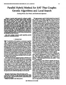
Fig. 3. Scale and wavelet symlets function for 32 coefficients
n∈Z
j
j
where a = 2 , b = k 2 , j ∈ N , k ∈ Z . The wavelet filter g plays the role of ψ [6]. The decomposition (filtering) process can be iterated, so that one signal is broken down into many lower resolution components. This is called the wavelet decomposition tree [6]. For detection of transients a multi-resolution analysis tree based on wavelets has been applied [7]. Every one of wavelet transform subbands is reconstructed separately from each other, so as to get k+1 separated components of a signal x[n]. The MATLAB multires function [8] calculates the approximation to the 2k scale and the detail signals from the 21 to the 2k scale for a given input signal. It uses the analysis filters H (lowpass) and G (highpass) and the synthesis filters RH and RG (lowpass and highpass respectively) (Fig. 2). As wavelet the symlets function was used. The symlets are nearly symmetrical wavelets proposed by Daubechies as modifications to the “db” family - orthogonal wavelets characterized by a maximal number of vanishing moments for some given support (Fig. 3).
V. METHOD OF SAG IDENTIFICATION WITH TRADITIONAL RMS VALUE BASED ALGORITHM Traditionally, in the power quality monitoring devices the tracking of RMS value of the voltage signal [1] is a sufficient indicator for the occurrence of a disturbance (sag or swell). Although this approach is robust and seen as a standard, for the DVR operation it is not fast enough. Some comparisons have been made to the other methods in use throughout the research activity. This is done by using the following equation
Vrms (k ) =
1 N
i =k
∑
vi 2
(36)
i = k − N +1
VI. RESEARCH RESULTS For experimental testing of the algorithms performance, a voltage dip generator was used that is capable of generating voltage dips of different magnitudes, duration and phase jumps A. Influence of Point on Wave The Point-on-Wave (Fig.4) corresponds to the instant of time of the voltage sinusoid signal when the voltage dip begins.
Fig. 2. Filters coefficients for symlets wavelet
Dips detection was realized through tracking values of details (D) representing higher frequencies in the signal. High
Fig. 4. Voltage dip characteristics
In Table I, the detection time (ms) using Kalman filter and Fourier based algorithms (using 1/8 cycle samples,) are shown
5 TABLE I INFLUENCE OF VOLTAGE DEPTH AND POINT ON WAVE RMS Residual voltage point on Kalman FFT magnitude [p.u] wave [deg] Detection Detection Detection time [ms] time [ms] Time [ms] (1/8 of cycle) samples
(Fig. 6). The results obtained with RMS tracking are also included (Fig. 5). Generally, dependence between point on
wave of the dip and detection time can be noticed. Dips starting when the voltage curve was in proximity of zero crossing were detected faster than voltage dip with an initial phase of 135 degrees. RMS tracking is significantly slower.
0
amplitude
0.2
0.2 0
0.5
-0.2 0.2
0.22
0.24 0.26 time [s]
0.28
0.3
0.8
0.08
rms
0.06
0,7 2,1 0 0,6 2,1 0,1 0,8 2,2 0,2 1,1 2,3 2,1
2,2 0,1 1,5 3,8 0,3
4,1 6,3 2,3 4,4 6,4 2,1 4,9 6,9 3,3 5,3 10,0 10,0
TABLE II WAVELET METHOD RESULTS
0.04 0.02 0.2
0.22
0.24 0.26 time [s]
0.28
0.3
Fig. 5. Time plot of the voltage under sag and computation of RMS value.
The voltage depth is another factor that has an important influence on the voltage dip detection algorithms. Both detection algorithms offer similar response. In general, for severe voltage dips (voltage depth 0.8 p.u. and residual voltage 0.2 p.u.) both detection algorithms are faster than for smaller ones.
amplitude [pu]
0,7 1,8 0,1 0,7 1,8 0,1
0 135 270 0 135 270 0 135 270 0 135 270
Residual voltage magnitue [p.u]
point on wave [deg]
0
135 270 135 270 135 270 135
0.2 0.5 0.8
Wavelet Symlet32
Wavelet Daub6
max/ mean 18.6884 25.2424 13.9072 17.2276 -10.4925 --
max/ mean 16.1074 -12.4587 -7.6045 ----
detection time 0.2599 0.2674 0.2599 0.2674 -0.2673 --
detection time 0.2572 -0.2573 -0.2572 ---
B. Influence of Phase angle jump From Fig.7 it can be deduced that the voltage magnitude during the dip, Udip, is:
0.15
u dip = 0.1
Z line Ethev Z line + Z thev
(1)
And the phase angle jump: arg(u dip ) = arctan
0.05
0
0.1
0.2 0.3 0.4 0.5 time [s] Fig. 6. Amplitude computation with Fourier based Algorithm (1/8 period)
Wavelet method delivered satisfactory results of beginning detection for signals shown in Table II. Compared with other methods the detection time is about 0.25 ms for all the signals analysed. For other signals this method did not perform well. Assumingly, higher order frequency components present in the signal deteriorated the detection ability. Two wavelets with significantly different lengths have been used; Symlet (length of the filter 32 samples) and Daub 6 (length of the filter 6 samples). The method, based on sudden change in the signal, rather than amplitude computation used the ratio of mean value of the first scale detail and the maximal value indicating sudden change (max/min, Table II).
X line X + X thev − arctan line Rline Rline + Rthev
(2)
Where Zline=(Rline+j·Xline) corresponds to the impedance of the fault, Zthev=(Rthev+j·Xthev) is the supply impedance and Ethev is the voltage supply.
Fig. 7. Diagram of the origin of voltage dips.
In distribution systems, Zthev, is typically composed by the transformer impedance with a large X/R ratio, while Zline is formed by cables with smaller X/R ratio. This will lead to a significant phase-angle jump during the dip. The detection algorithms have been compared considering different phase angle-jump during the voltage dip in two
6
situations: voltage depth 80% and 20%. Fourier based methods have been proved considering 1 /4 samples and 1/8 samples, (Table III). It is noted that the phase angle jump during the voltage dip affects the detection time, but in general the detection time is more affected by the voltage depth. Kalman filter and the Fourier based algorithms using 1/8 cycle samples offer very similar detection time results. The 1/4 cycle samples Fourier based algorithm does not offer any clear improvement. In some conditions the detection time is faster, but in other the detection time is much higher.
30
TABLE III INFLUENCE OF PHASE ANGLE JUMP Kalman FFT FFT Detection time (1/4 of cycle) (1/8 of cycle) [ms] samples. samples. Detection time Detection time [ms] [ms] 0,9 1,4 0,8
10 0 -30 -10 0 10 30 -30 -10
0,4 0,7 1 0,5 1,5 0,6 2,9 3,2 0,1
Residual Phase jump voltage magnitude [deg] [p.u] 0.2
0.8
0,1 1,6 1 1,1 3,9 0,6
0,3 0,6 1 0,5 1,1 0,4 2,2 2,5 0,2
C. Influence of frequency grid variation In practice, the power system frequency fluctuates around 50 Hz (Fig.8). For this reason, it is important to test the performance of the voltage dip estimation algorithms under frequency grid variations.
Fig. 8 Voltage dip measurement with frequency variation
Table IV shows the detection time employed by the different algorithms: Kalman filter, FFT (1/4 cycle samples) and FFT (1/8 cycle samples). It is noted that Fourier based algorithms using 1/8 cycle samples are the fastest. However, Kalman filter behaviour could have been improved by using a non linear extended Kalman filter, but the complexity is increased and consequently the final implementation on the DSP card becomes more complex. TABLE IV INFLUENCE OF FREQUENCY GRID VARIATION
Residual voltage magnitude [p.u]
Frequency grid [Hz]
Kalman Detection time [ms]
0,2
49.5 50 50,5 49.5 50 50,5
0,4 0,7 0,9 1,7 1,5 1,9
0,8
FFT (1/4 of cycle) samples. Detection time [ms] -0,9 1,5 -2,3 2,8
FFT (1/8 of cycle) samples. Detection time [ms] 0,3 0,6 0,8 0,9 1,1 1,1
VII. CONCLUSION Modern Power Electronic equipment for voltage dip mitigation requires fast and reliable detection algorithm. This paper has investigated several voltage dip detection algorithms such as Kalman filtering, Fourier based algorithms and Wavelets advanced processing signals. The performance of the amplitude estimations methods is compared in relation to the time it takes to each detection algorithm to estimate the beginning of the voltage dip. Wavelets method approach was different. Instead of amplitude estimation, details indicating higher frequency components were applied. This method was, however, prone to noise and other disturbances with higher frequencies components. Results from the study indicate that Kalman and Fourier based algorithms are able to respond within 1 ms for deep sags and swells, but for low voltage depth it takes up to 4 ms. This behaviour is acceptable according to the mitigation requirements since the voltage dips with largest magnitude require the fastest response. Popular RMS value tracking procedure underperforms. VIII. REFERENCES [1] M. H. J. Bollen, ‘‘Understanding Power Quality Problems: Voltage Sags and Interruptions’’. New York: IEEE Press, 1999, vol. I. [2] K.M. Tsang and W.L. Chan. ‘‘Simple, fast detector for voltage dip or voltage swell’’. ELECTRONICS LETTERS. February 2007 Vol. 43 No. 4. [3] J.E. Jipping, W. Ii. Carter, ‘‘Application and experience with a 15 kV static transfer switch’’, IEEE Transactions on Power Delivery, vol. 14, no. 4, October 1999, pp.1477 -1481. [4] E. Styvaktalcis , I.Y.H. Gu , M.H.J. Bollen ‘‘Voltage Dip Detection and Transients Power System’’, IEEE PES Summer Meeting, 2001.Vol 1, pp 683 688 [5] T. Lobos ‘‘Nonrecursive methods for real time determination of basic waveforms of voltages and currents’’ IEE PROCEEDINGS, vol. 136, Pt. C. No 6, November 1989. [6] M. Misiti, Y. Misity, G. Oppenheim, J-M. Poggi, ‘‘Wavelet Toolbox User’s Guide, MathWorks’’, 1996. [7] S. G. Mallat, ‘‘A theory of multiresolution signal decomposition: the wavelet representation", IEEE Trans. Pattern Analysis and Machine Intelligence’’, vol. PAMI 11, July 1998, pp. 647-693. [8] S.G. Sanchez, N.G. Prelcic, S.J.G. Galan, ‘‘Uvi Wave-Wavelet Toolbox for Matlab (ver 3.0)’’, University of Vigo,[Online]. Available: http://www.tsc.uvigo.es/~wavelets/uvi_wave.html, Apr. 1996