Computational Aeroelasticity of Rotating Wings with ... - FUN3d - NASA

Computational Aeroelasticity of Rotating Wings with Deformable Airfoils Smith Thepvongs

James R. Cook

Graduate Research Assistant

Graduate Research Assistant

[email protected]

[email protected]

Carlos E.S. Cesnik

Marilyn J. Smith

Professor

Associate Professor

[email protected]

[email protected]

Department of Aerospace Engineering School of Aerospace Engineering University of Michigan, Ann Arbor, MI Georgia Institute of Technology, Atlanta, GA Abstract This paper presents a simulation for high-fidelity aeroelastic analysis of rotating wings with camber-wise structural flexibility and embedded actuators. An unstructured Reynolds-Averaged Navier-Stokes (RANS) computational fluid dynamics (CFD) solver is coupled with a non-linear structural dynamics analysis. The CFD solution uses overset grids to combine the stationary and moving frames of reference. The structural formulation expands the conventional one-dimensional beam representation with additional degrees-of-freedom to capture plate-like cross-sectional deformations while allowing an arbitrary distribution of active and passive materials in the cross section. Motion and forces on the non-coincident fluid and structural grids are transferred using a finite-element-based interpolation, along with a least-squares fit for extrapolations. Trim and convergence to periodic response are assisted by a low-order analysis that is also discussed. Finally, as an initial verification of the implementations, results from the low-order and CFD-based solutions are compared for a rigid-airfoil rotor in forward flight.

Introduction Reducing noise, vibration and power consumption is becoming increasingly important to the modern helicopter industry. This has inspired the development of many new technologies. Especially promising are those based on active blade control which have a potential ability to adapt to flight conditions as well as improve multiple characteristics through the same system. Such concepts have traditionally achieved control without intentionally deforming the airfoil’s main supporting structure. Recently Presented at the American Helicopter Society 65th Annual Forum, Grapevine, Texas, May 27-29, c 2009. Copyright °2009 by the American Helicopter Society, Inc. All rights reserved.

however, actuation systems have been proposed that apply continuous shape changes through the use of integrated active materials [1, 2]. These morphingtype systems may offer several benefits, including improved aerodynamic efficiency as well as potential for good structural weight efficiency if the actuators themselves contribute to blade overall stiffness and strength. Although some aspects of these systems have been previously studied, general design requirements and effectiveness are still largely unknown. In order to analyze morphing-type rotors in depth, one must consider several phenomena normally assumed to be unimportant in rotor problems. Structurally, shape changes can be introduced by a combination of cross-section flexibility and actuator forces. Bending along the chordline cannot be modeled in the beam formulations typically used for rotor analyses, while the coupled actuator/structural

dynamics may be difficult to analyze when the actuator is highly integrated. Aerodynamically, the possibility of general conformations adds a large degree of complexity. Besides altering the behavior associated with linear phenomena, shape changes can also signficantly change the effects of compressibility or viscosity. To properly assess the impact on vibration and power, these higher-order effects must be considered. In the modern aeroelastic analysis of rotors, nondeforming cross sections are generally assumed in the structural and aerodynamics theories, as well as in their coupling. The structural theories are based on classical beam degrees-of-freedom, and the aerodynamics use either a lifting line model (often augmented with semi-empirical models to account for higher-order effects), or computational fluid dynamics. For the latter, the current state-of-the-art is Reynolds-Averaged Navier Stokes (RANS). Examples of the successful coupling of structural dynamics analyses with RANS-CFD include CAMRADOVERFLOW [3], DYMORE-OVERFLOW [4], RCAS-OVERFLOW [5], UMARC-TURNS [6], and HOST-elsA [7]. Though significant progress has been made in CFD-based aeroelastic simulation, the ability to model deformable airfoils (with or without actuation) while also having sufficient accuracy for noise, vibration and power assessment has not been developed to the authors’ knowledge. This paper describes the development of a highfidelity simulation for the aeroelastic analysis of rotors with actuated, flexible airfoils. The simulation consists of a RANS CFD analysis coupled threedimensionally with a structural analysis that captures camber deformations. The simulation is supported by a finite-state, semi-empirical aerodynamics analysis, which is used to assist initialization and trim. The theories and coupling strategies of the different formulations are presented. A preliminary comparison of the aeroelastic response predictions from the low-order and CFD-based analyses is also shown for a rotor in forward flight.

Structural Dynamics Formulation The computational structurual dynamics (CSD) formulation used in the current study has been presented in Refs. 8 and 9. It follows the variationalasymptotic method for the analysis of composite beams [10]; that is, the equations of motion

for a slender anisotropic elastic three-dimensional solid are approximated by the recursive solution of a linear two-dimensional problem at each cross section [9], and a one-dimensional geometricallynonlinear problem along the reference line [8]. This procedure allows the asymptotic approximation of the three-dimensional warping field in the beam cross sections, which are used with the one-dimensional beam solution to recover a threedimensional displacement field. The present implementation adds an arbitrary expansion of the displacement field through a set of functions approximating the sectional deformation field to capture “non-classical” deformations, which are referred to as finite-section modes. The geometrically-nonlinear dynamic equations of equilibrium along a reference line of a slender solid were presented in Ref. 8. If all magnitudes are expressed in their components in a reference frame attached to the deformed reference line, they are written as: d ˜ B )PB = ( d + KB )(FB − f1 ) + f0 +Ω dt dx d ˜ B )HB + VB PB = ( +Ω dt d + KB )(MB − m1 ) + (˜ e1 + γ˜ )FB + m0 ( dx d d Qt = (Qs1 − fs1 − (Qs0 − fs0 ) dt dx

(

(1) The first two sets of equations imply equilibrium of forces and moments, where K is the current curvature of the reference line, the pairs (V, Ω) and (P, H) are the local translational and rotational inertial velocities and momenta, respectively, and F and M are the sectional forces and moments (similar to traditional geometric-nonlinear blade modeling in state-of-the-art rotorcraft aeromechanics codes). In addition, f0 and m0 are the conventional (zeroorder) applied forces and moments, respectively, per unit length on the beam, while f1 and m1 are the first-order loads associated to the work needed to deform the cross section. The last set of equations includes the equilibrium of the generalized forces (Qs0 , Qs1 ) and momenta, Qt , corresponding to the finite-section modes, which are defined by prescribed cross-sectional displacement shapes ψq (x2 , x3 ) with amplitude q(x). These equations are complemented by the cross-sectional constitutive relations, which, for a elastic solid with embedded ac-

tuation, are derived in Ref. 8 using the variationalasymptotic method. These equations take the final form of  FB    MB Qs0    Qs1   PB HB  Qt

    γ          κ − = [S]       q0        q      VB  ΩB = [M ]    q˙    

F (a) M (a) (a) Qs0 (a) Qs1

h(ξ) = Z

    

∞ X

hn Tn (ξ)

n=0 1

Ln = −b

Tn (ξ)∆P dξ

(3)

−1

    (2)

where [S] and [M ] are the cross-sectional stiffness and mass matrices, respectively. The superscript (a) indicates actuation loads per unit length on the structure, and γ and κ are the beam strain measures associated to forces and moments, respectively. The variational asymptotic method determines [S], [M ] and actuation loads by discretizing the cross section into finite elements, allowing an arbitrary geometry and material distribution. To develop a finite-element solution, the dynamics of the member are first described by a mixed formulation in which the variation of the equations of virtual work are taken with regard to displacement, force and momentum variables. These variables are used to define the structural state. Straindisplacement relations and velocity-displacement relations are satisfied simultaneously by using Lagrange multipliers. The resulting governing equations are first-order in time and space, which allows the use of simple integration schemes. The solution of these equations has been implemented in the computer code UM/NLABS (University of Michigan’s Nonlinear Active Beam Solver).

Low-Order Aerodynamics Formulation Deforming Thin-Airfoil Theory The low-order model uses the two-dimensional finite-state formulation for flexible airfoils presented in Ref. 11. It is based on a Glauert expansion of the potential flow equations for a deformable airfoil of infinitesimal thickness. The camber-wise airfoil deformation is written as:

where h is the local displacement normal to the chord, b is the semi-chord length and ξ is the nondimensional coordinate along the chordwise direction. Tn are the Chebyshev polynomials of the first kind, which define the generalized camber-wise displacement amplitudes, hn , and its associated airloads, Ln integrated from the local airloads ∆P . The final result (Ref. 11) for the airloads computed in the normal and chord directions arising from the potential flow assumptions is: 1 ¯ L ρc`α

¨¯ + ν¯˙ ) = −b2 M (h ¯ ¯˙ + ν¯ − λ ¯ 0 ) − u2 K h −bu0 C(h 0 ¯ ¯ −bG(u˙ 0 h − u0 ν¯ − u0 λ0 )

1 ¯ D0 ρc`α

(4)

¯˙ + ν¯ − λ ¯ 0 )T S(h ¯˙ + ν¯ − λ ¯0) = −b(h ¨¯ + ν¯˙ )T Gh ¯ +b(h ¯˙ + ν¯ − λ ¯ 0 )T (K − H)h ¯ −u0 (h T ¯ ¯ ¯ +(u˙ 0 h − u0 ν¯ + u0 λ0 ) H h

¯ = L ν¯ = ¯ λ0 =

{L0 , L1 , Ln , ...}T {ν0 , ν1 , 0, ...}T {λ0 , 0, 0, ...}T

(5)

(6)

¯ is the vector containing the generalized airwhere L loads, and similar definitions are given for the gener¯ rigid-section alized camber-wise displacements (h), normal velocity (¯ ν ), and section inflow distribution ¯ (λ). The drag force is D0 , and M, S, G, K, and H are constant coefficient matrices whose complete definition is given in Ref. 11.

Dynamic Wake The wake-induced velocity (λ0 in eqn. 6) is solved using the dynamic inflow theory of Ref. 12. It assumes that the velocity normal to the rotor disk can

be expressed in terms of the radial and azimuthal expansion functions,

w(s, ψ, t) =

∞ X

∞ X

φrj (s) ×

tion, the total airloads can be expressed as: 1

D0,tot

= D0 + ρbcd (u20 + ν¯T S ν¯) 2 u0

L0,tot L1,tot

= L0 − ρbcd (u20 + ν¯T S ν¯) 2 S ν¯ + ρu0 Γ0 = L1 + +ρu0 Γ1 (10)

1

r=0 j=r+1,r+ψ,...

£ r ¤ αj (t)cos(rψ) + βjr (t)sin(rψ)

(7)

where s and t are the non-dimensionalized radius and time, while ψ is the azimuth. The inflow states, α and β, are coefficients of terms containing the product of azimuthal harmonics and radial expansion functions φ, indexed by r and j, respectively. The governing equations for the inflow states are given by: 1 mc {τ } 2 n £ 1¤ r 1 M {β˙ j } + [Ls ]−1 {βjr } = {τnms } 2 [M 1 ]{α˙ jr } + [Lc ]−1 {αjr } =

(8)

The pressure coefficients, τ , are determined from the circulatory lift, which is available from eqn. 4 by neglecting terms associated to accelerations in the zeroth-order loading. The left hand side coefficient matrices, [M 1 ] and [Lc,s ] are determined by the wake skew angle. Finally, with the solution of the inflow states, the zeroth-order inflow (λ0 ) is calculated from: µ ¶ ∞ ∞ X X rb λ0 = J0 φrj (s) × s r=0 j=r+1,r+3,... £ r ¤ αj (t)cos(rψ) + βjr (t)sin(rψ) (9) where J0 is the Bessel function of the first kind and can be approximated by taking the first few terms in its series.

Drag and Dynamic Stall A potential benefit of camber actuation is the ability to alter profile drag and stall characteristics, which have implications in power and vibration. To include these effects in the low-order model, the potential-flow airload expressions are augmented with a quasi-static profile drag term as well as a dynamic-stall correction that is based on the ONERA model [13], taking the approach described in Stumpf and Peters [14]. In the current implementa-

where cd is the profile drag coefficient, Γ0 and Γ1 are the dynamic stall states corresponding to the zeroth and first-order generalized loads, respectively. The ONERA model assumes that the dynamic stall states are governed by a second-order differential equation, and requires static loading coefficients near and beyond stall. These, along with cd , are determined using the two-dimensional boundary layer analysis code XFOIL [15] (which is valid to justafter-stall), along with a simple, empirically-derived approximation for deep-stall. The coefficients are obtained under varying Reynolds number, angle-ofattack and camber deformation. A detailed account of the method used for determining the coefficients is available in Thepvongs et. al [16].

Coupling with Finite-State Aerodynamics The finite-state aerodynamics formulation uses Chebyshev polynomials to form a basis for the camber deformations and associated airloads, while the choice of basis functions for the finite-section modes are arbitrary. The motion and force variables of the aerodynamics formulation are related to those of the structural formulation by a simple linear expression, as derived in Thepvongs et. al [16]. This straightforward connection between the aerodynamic and structural states allows the same space and time integration methods to be used for both formulations as well as a simultaneous solution. The governing structural dynamics equations (eqn. 1), aerodynamic load expressions (eqns. 4, 5), dynamic stall equations and wake equations (eqn. 8) together define the time-domain problem. An explicit method is used with iterative refinement to achieve the desired convergence. Consider the following form of the structural dynamics equations, obtained by applying spatial discretization (finiteelements) to eqn. 1. The set of differential-algebraic equations, along with the appropriate set of boundary conditions can be written as:

ˆp) A(Xp )X˙ p + S(Xp , X ˆp) BC(X

ˆp, = LF S (Xp , X˙ p , X ¯p) α |p , β |p , Γ = 0

(11)

where A is the inertia matrix operator, S is the structural matrix operator, written as functions of the structural state vector, X , its time derivative, ˙ and boundary values, X. ˆ These, along with the X, aerodynamic states, are all obtained at the current time (time is indexed by p). The load matrix operator LF S is the contribution of the aerodynamic loading which is a function of the structural, inflow, and dynamic stall states. A simple three-point backwards Euler timeintegration scheme is used in accordance with the first-order form of the structural and potential flow ¨¯ term of eqn. 4 is obtained governing equations (the h by first derivatives of the velocity, which is a structural state variable due to the mixed formulation). A four-point scheme is used to integrate the secondorder dynamic stall equations. The time-integration formulas are:

˙ = 3()p − 4()p−1 + 1()p−2 () p 2∆t 2() − 5() + 4() p p−1 p−2 − 1()p−3 ¨ = () p (∆t)2

τ θ¨ + θ˙

=

Jkl

≈

J −1 {a(G − g) − bg˙ − d¨ g} Z 1 T ∂gk dt T 0 ∂θ1

where θ = [ θ0 θ1c θ1s ]T is the control settings, and G and g are the target and current values of the variables representing equilibrium (i.e., the thrust, pitch and roll moments), respectively. For the test cases run in this study, coefficients b, d, and τ are set to zero, and a = 1/T , where T is the period. The ”trimmability matrix” J can be approximated by numerically-computed Jacobian, determined by stepping the controls and examining the response at an instant one revolution later. It should be noted that the trim is solved externally to the aerodynamic and structural equations, using the time integration scheme of eqn. 12. Since the body loads are computed from structural variables, namely the root reaction loads, the trim is independent of the aerodynamics. Thus, the same trim algorithm and implementation is used for the low-order and CFDbased analyses.

High-Fidelity Formulation (12)

The nonlinear system is solved, along with the boundary conditions of eqn. 11 by Newton-Raphson iterations, with the Jacobians of the left-hand side operators of eqn. 11 available in closed form.

Trim The enforcement of vehicle equilibrium adds more variables and constraints to the aeroelastic problem. The present work assumes a wind-tunnel setup, where the variables are taken to be the collective, sine and cosine components of the cyclic pitch, and equilibrium is represented by specifying values for the time-averaged thrust, pitch and roll moments. An auto-pilot method has been described by Peters et. al [17], which makes incremental changes to the control settings at every timestep. The control settings are governed by:

(13)

Aerodynamics

Unstructured or mixed-element CFD methods have advantages over structured-based CFD methods that can be exploited for rotorcraft analysis. In particular, rapid grid generation for complex configurations is usually cited as a major reduction in the preprocessing stage. Additional advantages exist because unstructured methods can model rotors with fewer overset grids, resulting in less computational expenditure for grid motion and potentially a reduction in numerical errors via fringe and orphan computations. The most physically correct analysis requires that all surfaces be accurately modeled via the time-accurate Navier-Stokes equations, requiring that two frames of motion be modeled during a single simulation. While several options exist, one of the most applied approaches utilizes a combination of overset grids to generate smaller grids around each rotor blade, which then rotate through a background grid that may include a fuselage, ground planes, or other important configurations. This overset approach has been used to correctly capture the general experimental trends on several configurations by Hariharan [18], Potsdam et

al [3] and Duque et. al [19], O’Brien and Smith [20] and Abras and Smith [21]. Because of the potential of the unstructured methodologies for advanced rotor configurations, as well as their ability to rapidly model rotor vehicle components, an unstructured methodology has been chosen to provide the aerodynamic simulation for this effort. The unstructured methodology selected for this effort is the FUN3D code developed at the NASA Langley Research Center [22–24]. FUN3D can resolve either the compressible or incompressible RANS equations on unstructured tetrahedral or mixed element meshes. The incompressible RANS equations are simulated via Chorin’s artificial compressibility method [25]. A first-order backward Euler scheme with local time stepping has been applied to steady-state applications, while a second-order backward differentiation formula (BDF) has been utilized for time-accurate simulations. A pointimplicit relaxation scheme resolves the resulting linearized system of equations. The RANS equations are resolved via non-overlapping control volumes surrounding each cell vertex or node where the flow variables are stored. Inviscid fluxes on the cell faces are solved via Roe’s scheme [26] that splits the flux differences. The viscous fluxes are computed with a finite volume formulation to obtain an equivalent central-difference approximation. The FUN3D methodology was originally developed for fixed-wing applications by NASA researchers. Georgia Tech researchers have extended it for rotary-wing applications of interest, as described by O’Brien and Smith [20] and Abras and Smith [21]. O’Brien [27] has shown that FUN3D’s steady incompressible formulation is not only robust for low-speed flight regimes, but both compressible and incompressible results comparable to structured methods are obtained when the grids are locally comparable on the surface and boundary layers. In addition, O’Brien developed an overset formulation of FUN3D to handle mixed inertial-moving frames necessary to model rotating wings. This formulation makes use of the DiRTLib [28] and SUGGAR [29] libraries to compute the cell connectivity and provide the hole cutting necessary with moving frames. Abras [30] has extended the FUN3D code further to provide full rotor articulation, as well as loosecoupling with a computational structural dynamics code, assuming that the rotor is modeled as a structural beam. These extensions form the basis for the three-dimensional aeroelastic rotating wing simulations, extended further to include camber deformations.

Modifications for Aeroelastic Coupling While many of the components necessary to perform rotating, overset computations were extended by prior Georgia Tech researchers, there remained a number of modifications that were necessary to accomplish full surface deflections within a tightlycoupled framework. FUN3D is capable of handling multiple grids to define the rotor blade and, as a massively parallel simulation methodology, will decompose each grid further as it parses the computational load among a number of processors. The current coupling scheme uses subdivisions of the blade surface nodes, dividing them into smaller groups (as later described). In order to couple FUN3D, the nodes of each of the blade surfaces in FUN3D must be identified and sorted into the groups. The blade local coordinates of the surface nodes in FUN3D are collected from each processor. The CFD nodes that define the edges of the groups may belong to more than one group, so the nodes are flagged to ensure that the same surface node is not passed to included in the coupling more than once. Another array containing the coordinates of the surface face centers is created and sorted in the same way. As is the case with most CFD solvers, FUN3D resolves the primitive variables of the flowfield using a nondimensional system. NLABS, as is typical for CSD solvers, uses dimensional quantities. Thus, the pressure coefficient on each cell face that lies on the blade surface is computed within the CFD code, and are then dimensionalized using the freestream pressure of the simulation. Similarly, spatial coordinates of each cell are dimensionalized and the area of the CFD cell computed, so that a dimensional force is computed from the cell pressure and area. This force array is passed into NLABS, which finds the structural deflections at each node location and passes the new coordinates back to FUN3D, along with the orientation of the blade. For the coupling, it is necessary to deform not only the CFD surface, but also the CFD volume grid. As illustrated in Refs. 21 and 30, large surface deflections from not only the elasticity of the blade but new trim or articulation commands can cause the blade near-body grid to encounter poor cell resolution. In order the minimize the volume grid deformation, the elastic deflection of the blade is included in the Euler angle rotations. For example, in this application, the pitch angle is defined as the control pitch angle plus 0.5 times the elastic

twist of the blade at the tip. Flap and lead/lag angles are defined using a straight line extending from the elastic axis at the root to the location of the elastic axis of the tip. Using the deformations and any control changes from NLABS, the pitch, flap, and lead/lag angles are extracted and updated in the six degree-of -freedom motion equation. The remaining elastic deformations are then applied to the rotor surface. The near-field volume grid based on the new surface node coordinates is then generated, and the SUGGAR library [29] is then accessed to calculate new connectivity data. At this point the flow solver is allowed to advance to a new time step at which point the process is repeated.

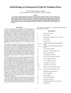
Figure 1: Simulation flow.

Time Coupling and Initialization

loads are set to gradually transition from those of the low-order model to those of the CFD in order to prevent disturbances that may be slow to decay.

Due to its computational cost, the CFD-based analysis uses a weaker coupling of the fluid and structural solutions compared to that of the loworder model. Any coupling scheme that needs repeated solutions of the CFD or modification of the CFD boundary conditions during a timestep would not likely be affordable. Instead, the current approach obtains separate solutions for the CFD and CSD analyses, where, within a given timestep, the computed state of one is held fixed during the solution of the other, using the most-recently available information and no subiterations. It has been demonstrated by prior work [31, 32] that for hover and forward flight that a loose-coupling between the CFD and CSD codes is sufficient. Further, fixedwing researchers, (e.g. Refs. 33, 34), have shown that for the small time step size needed for a stable (uncoupled) CFD solution, that the resulting errors are negligible. To further reduce computational time, the loworder aerodynamics model supports the initialization and trimming of the CFD-based aeroelastic analysis. Long-time simulations are required for computation of the trim Jacobian and convergence to a sufficiently periodic and trimmed response. The low-order model can be used to compute the Jacobian and provide a starting condition of the CFDbased analysis. The starting condition is obtained by allowing the low-order model to run to convergence, then extracting the structural state and control settings. These are used to initialize the CFD-based analysis, which is run with the low-order model kept activated. The applied aerodynamic

The time-coupling scheme described above is formalized by augmenting eqn. 11 so that the scheme becomes:

ˆp) = A(Xp )X˙ p + S(Xp , X ˆ p−1 ) ζLCF D (Xp−1 , X˙ p−1 , X +(1 − ζ)LF S

(14)

where LCF D represents the numerically-computed (non-linear) CFD loads (transformed and integrated to structural forcing variables, as described in the following section) and ζ is the weighting factor that controls the transition between the CFD and loworder loads (0 ≤ ζ ≤ 1). A diagram showing the general operation of the combined aeroelastic simulation is shown in Fig. 1.

Transformation of Structure Variables

Fluid

–

The fluid and structure wetted surfaces are discretized separately according to the resolution requirements of the individual analyses. Therefore a transformation is needed to properly connect the motion and force variables between the two. This transformation has to consider the presence of camber-wise flexibility in addition to the usual beam degrees-of-freedom. Although the finite section modes are treated as one-dimensional beam variables, they are defined in a discrete way within

the cross-section analysis. This is accomplished by specifying the modes’ contribution to the displacement at a selected number of grid points within the cross section (which are a subset of the total grid points used to discretize the cross-section problem). Additionally, the motion of these crosssection grid points is determined partly by warping arising from sources other than the finite-section modes. For these reasons, quantities at the CFD grid cannot be directly expressed by (or integrated to) one-dimensional beam variables, as is often done when coupling CFD to conventional beam analyses [31, 32]. An intermediate step involving the threedimensional structural grid is required. From this three-dimensional structural grid, the displacements are interpolated to the CFD grid finite-element shape functions, as originally described by Pidaparti [35] and extended by [37]. A triangulation of the structural grid points forms a new set of elements which are used solely for the interface. Next, for each structural interface element, all enclosed CFD nodes are identified. The criterion for enclosure is that there exists a vector normal to the element that intersects both the element and the grid point. Among the structural interface elements meeting this criterion, the one having the shortest distance to the CFD node is used for interpolation. D The displacement of this CFD node, uCF , is dej fined by: D uCF = Nj uCSD + Rdj j i

(15)

uCSD i

is the column matrix of the displacewhere ments at the nodes of the structural interface element i, and Nj is the row matrix containing the element shape functions evaluated at the CFD node. The shape functions are linear for the 3-node element. The last term in the above equation accounts for separation between the CFD node and the element plane. It preserves the separation distance and CFD node’s local coordinate within the element throughout the deformation. The vector from the element plane to the CFD node is dj , and the matrix rotating the element normal from its undeformed to deformed orientation is R. The transformation of the forces from the CFD cell centers to the structural interface mesh uses the same finite-element shape functions. The force at a CFD cell, FkCF D , is distributed to the nodes of the enclosing structural interface element by the relation:

FiCSD = NkT FkCF D

(16)

where Nk represents shape functions evalutated at the cell center position k. Some CFD nodes may not be enclosed by a structural interface element due to the boundaries of the CFD and CSD grids being slightly offset. The present study attempts to model the same geometry (the wetted surface) in each analysis, therefore the offset is caused only by the different discretizations in each grid or numerical precision errors. For the displacement of these points, extrapolation is performed using a function fitted to the structural interface grid:

D = uCF j

P X £ ¤1 D 2 − xCF ) + r2 2 γji (xCSD i j

(17)

i=1 D are the position of the strucwhere xCSD and xCF i j tural and fluid nodes, respectively. P is the total number of structural nodes over which the extrapolation function is formed, r is a shape parameter (Ref. 36) and γji are the computed weighting coefficients. Following the extrapolation, the displacements of these points are averaged with its neighbors to improve smoothness between interpolated and extrapolated regions. Forces originating from CFD cell centers not enclosed by any element are simply lumped along with its moment contribution to the nearest structural node.

In the current study, the CSD and CFD meshes are subdivided into four domains, corresponding to the tip, root, top and bottom surfaces of the blade. The interpolations (specifically, the searching) and extrapolations are done separately for each domain to reduce overall computational costs. The interpolation and extrapolation algorithms described above are implemented in modified versions of the work by authors of Refs. 36 and 37. It should be mentioned that the fluid and structural problems should ideally form a closed system, as discussed by Smith [38]. The right-most term of eqn. 15, which has been added as part of the current work, removes the conservation of work across the interface that normally occurs with finite-elementbased interpolation. This term, however, improved accuracy of the interpolations when the separation distance between the CFD nodes and its enclosing element became large, as discussed in the next section. Similarly, the method of extrapolation and integrating forces for unenclosed CFD nodes does

not enforce conservation of work. Errors resulting from the addition/loss of energy through the transformations are presumed to be small. This should be further investigated, however, in future studies.

Numerical Investigation: Rotor Model and Discretization Results presented in this study are based on a scaled BO105 rotor model. The rotor is hingeless, 4-bladed, and has a 2-m tip radius. From 0.44R to the tip, the blade has a 0.121-m chord and an NACA 23012 airfoil, modified with a trailing-edge tab. The rotation speed is 109 rad/s. The CFD blade surface grid (Fig. 2) was constructed from the detailed geometry provided in Ref. 39. The moving-volume grid forms a rectangular prism that encloses the region between 1-chord length inboard of the root-most blade edge to 2chord lengths beyond the tip, 1-chord length ahead of the leading edge to 1-chord length behind the trailing edge, and 2-chord lengths below the blade to 2-chord lenghts above it. A total of 896,241 nodes are contained in the moving-volume grid of each blade. The background grid is a cylinder extending 40 m above and below the rotor, with a diameter of 80 m, and is comprised of 1,046,807 nodes. The CSD discretization is defined by the distribution of finite-element nodes along the beam reference line, along with grid points within the crosssections at those nodes. For the reference line, there are 43 elements, concentrated near the transition region. Each cross section contains 80 grid points, distributed along the wetted surface and concentrated near the leading and trailing edges. These grid points and their triangulation for the fluid-structure interface is shown in Fig. 3. A summary of the fluid and structural discretizations is given in Table 1. For the cross-section properties, integrated mass and stiffness data for the conventional beam degrees-of-freedom were available, however, detailed layup information could not be obtained. The finitesection mass and stiffness were set to values [16] that prevented significant camber deformation due to aerodynamic loads or dynamic response. This created a realistic condition for the initial validation of the simulations.

(a) CFD surface grid

(b) Near-field blade grid

(c) Full CFD volume grid

Figure 2: CFD grids for the BO105 rotor.

Figure 3: CSD mesh for the BO105 rotor.

Table 1: Blade discretization summary (per blade). CFD surface nodes CFD surface cells Structural interface nodes Structural interface cells Structural 1-D elements

Figure 4: Test load magnitude (N ) at discrete points on CFD grid.

20398 40972 3680 6864 43

Numerical Investigation: sults

Re-

Verification of the Fluid – Structure Transformation The basic methodology of the interface algorithms has already been validated for a set of canonical cases, as presented by Lee [37]. Several aspects of the interface are re-examined, using the grids for the BO105 model currently being studied. To verify the transformation of forces, a load was prescribed at the CFD cell centers that varied substantially in amplitude and orientation. Fig. 4 shows the distribution of the amplitude along the top and root surfaces. These forces were then transferred to the structural nodes through the interface, and integrated to find the total forces and moments acting on the blade (the latter about the hub center). Under this loading, the error in the global forces along the three axes was found to be less than 1 × 10−12 % and for the moments, less than 0.01%. A visual approach was employed to verify the displacement transformations. A sample displacement field was set up by applying transverse and finite-section (camber-wise bending) forces along the structure, producing large displacements. Fig. 5 shows the co-movement of the fluid and structural wetted-surface nodes. The necessity of the rotational term in the in-

Figure 5: Sample undeformed and deformed grids including camber-wise bending response – small points: CFD; large points: structural interface. terpolation scheme of Eqn. 15 is demonstrated in Fig. 6. Because the CSD grid is substantially coarser than that of the CFD, the CFD-node-to-interfaceelement distance can become large when there is discontinuous geometry in the CFD grid. An example is the transition region of the blade, near the trailing-edge tab. Fig. 6 shows this region, where the view is from the root towards the tip, as indicated by the arrow in Fig. 2(a). A 20◦ rigid-body pitch rotation is applied to the structure, and the interface transforms the CFD mesh shown in Fig. 6(a). The rotational term in the interpolation equations preserves the shape of the mesh (Fig. 6(b)), while neglecting the term causes the surface to become wrinkled (Fig. 6(c)).

Forward Flight With verification of the fluid-structural interface, several characteristics of the aeroelastic response are examined for a forward-flight condition. The advance ratio considered is 0.25, and the shaft angle is −5◦ . Following the wind-tunnel experiments of Ref. 39, the trim condition is 3100N thrust (Fz ), zero pitching moment (My ) and zero rolling moment

(Mx ), evaluated as time-averaged quantities. In the first set of results, the effect of the transition length between the low-order and CFD loads is examined. Three time functions are setup for the variation of (ζ) in Eq. 14. The first is a step function, while the second two increase linearly from 0 to 1, over a half and full revolution. In the following figures, the first revolution contains the response computed by the low-order analysis after its convergence to periodicity and trim. After this revolution, the CFD solution begins along with the transition from the low-order to CFD loads, using one of the three transition methods.

(a) Original

(b) With rotational term

(c) Without rotational term

Figure 6: CFD grid near trailing edge of transition region; a) original; 20 deg. pitch applied through fluid-structure interface with (b) and without (c) rotational term in Eqn. 15.

Figure 7 shows the time-history of the instantaneous, fixed-frame hub loads, while Fig. 8 shows the control settings. Comparing the converged control settings of the low-order and CFD-based analyses (Table 2), there is a 0.6◦ difference in the collective, while the cosine and sine components differ by 0.2◦ and 0.3◦ , respectively. The step transition from loworder to CFD loads produces the largest deviation from the previously-established equilibrium. This deviation is reduced by the half-revolution ramp, then further by the full-revolution ramp. Despite this perturbation, the convergence of both the control settings and hub loads appear to take less time overall using the step transition. In examining the control settings, the collective changes at a faster rate with the step transition while also appearing to have a head start compared to the other transition methods. The sine and cosine components of the pitch control also show earlier arrival at the converged value, although the rate appears to be unaffected by the transition method. These results suggests that allowing the trim algorithm to act earlier on the CFD-based aeroelastic response is more important than avoiding disturbances caused by sudden transitioning. In other words, the damping (which is dominated by aerodynamic loading) is sufficient to decay the disturbances such that they are insignificant well before trim is reached. Table 2: Control settings in degrees at convergence of trim and aeroelastic response.

θ0 θ1c θ1s

The

second

CFD 10.8 0.7 -2.5

set

of

Low-order 10.2 0.857 -2.82

results

compare

the

CFD

Low−order

x

F (N)

100

θ1s (deg.)

0.5

1.0 revs.

F (N)

y

10.5 10 1

Fz (N)

0 −2.5 −3 0

1

2

0.0

3 4 Revolutions

5

6

7

0.5

1.0 revs.

Fz (N)

3500

Mx (Nm)

3100 3000

Figure 7: Pitch control history, varying length of transition between low-order and CFD loads.

3000 2500 2000 100 0 −100 −200

My (Nm)

0 −200 3200

0.5

−3.5

0 −100 200

11

θ1c (deg.)

θ0 (deg.)

0.0

0 −100 −200 0

1

2

3 4 Revolutions

5

6

7

Figure 8: Hub loads history, varying length of transition between low-order and CFD loads.

0

0.25

0.5 Revolutions

0.75

1

Figure 9: Hub forces comparison of converged loworder and CFD predictions. periodically-converged, trimmed responses of the low-order and CFD analyses as an attempt to co-validate them. The fixed-frame hub forces are shown in Fig. 9, while the moments are shown in Fig. 10. The rearward and starboard-side loads, Fx and Fy , show good agreement in frequency and phase of the response, though significant differences are seen in the amplitudes, as well as the mean value of Fy relative to its amplitude. As expected, the mean values of Fz , Mx , and My approach the values enforced by the trim algorithm, however, large differences can be seen in most other aspects of the time response. Also, in the torque (Mz ), the low-order prediction of the magnitude of the mean value is 13% smaller than that of the CFD which if uncoupled from the other errors, may indicate that improvements in the drag model are needed. Lastly, it is important to note that for all of the fixed-frame loads, the CFD generally predicts a larger vibratory amplitude. The tip deflections are presented in Fig. 11. The chordwise (positive in the leading direction), flapwise (positive up) and pitchwise (positive nose up) responses are shown. Several similarities can be seen in the predictions from the two analyses. In the chordwise response, both results show a dominant 1/rev component and a similar phase. The CFD loads produce a larger mean deflection in the lag direction, which agrees with the larger torque magnitude found in the hub loads. The flapwise response also shows agreement in several aspects. The positive peak occurs near 270◦ azimuth (0.75 of the

Low−order

CFD flapwise (m) chordwise (m)

CFD Mx (Nm)

100 0

0

−50 −300 −350 −400

−0.015 −0.02

pitch (deg.)

Mz (Nm)

My (Nm)

−100 50

0

0.25

0.5 Revolutions

0.75

1

Low−order

0.08 0.06 0.04 6 4 2 0 −2

0

0.25

0.5 Revolutions

0.75

1

Figure 10: Hub moments comparison of low-order (converged) and CFD (latest rotation available) predictions.

Figure 11: Tip deflections comparison of low-order (converged) and CFD (latest rotation available) predictions.

revolution), while a flat response is seen near 0◦ azimuth. The CFD loads, however, appear to induce a more significant 3/rev component than those of the low-order model. The mean values from both predictions are similar. In the pitchwise response, the absolute rotation is shown (includes both elastic and rigid-body contributions). The CFD predicts a more negative overall rotation at the tip, despite the increased collective pitch. This suggests that a larger nose-down aerodynamic pitching moment is computed by the CFD analysis, and this may be the source of the requirement for increased collective pitch.

which has been parallelized, is pending and should improve the execution speed. The combined loworder aerodynamics, structures and fluid-structure transformations take several seconds of serial computations for each time step.

Despite the differences in the aeroelastic response predicted by the two aerodynamics models, correlation in several aspects including control settings, tip flapwise response and some hub loads, appear to verify a correct implementation, especially given the vastly different approaches used in coupling the analyses.

Computational Requirements The coupled code is executed on a cluster of IBM Power5+ 1.9 GHz processors. For the high-fidelity analysis, a total of 64 processors have been used: 63 for the parallel FUN3D computations and one for the serial computations which includes NLABS and SUGGAR. Execution takes about 4.5 minutes per time step (about 27 hours per revolution). It should be noted that a new version of SUGGAR,

Concluding Remarks A simulation for high-fidelity analysis of rotors with actuated, flexible airfoils has been presented. It includes a quasi-three-dimensional CSD analysis, RANS CFD (FUN3D) analysis, as well as coupling, trim and initialization algorithms. Results were presented for a scaled BO105 rotor that explored several aspects of the coupling in addition to the general time response. When using a low-order aerodynamics model for initializing the structural state and control settings, a sudden transition between the low-order and CFD-based loads was found to produce faster convergence to a periodic, trimmed solution compared to that produced by a gradual transition. A comparison of the aeroelastic response predicted by the low-order aerodynamics model and CFD showed agreement in trimmed control settings, as well as aspects of the tip deflections and fixedframe hub-loads. Although further validations are needed, these results serve as a basic verification of the methodology for coupling FUN3D with the three-dimensional CSD analysis.

Acknowledgments This work is sponsored by the National Rotorcraft Technology Center (NTRC) Vertical Lift/Rotorcraft Center of Excellence (VLRCOE) at the Georgia Institute of Technology and University of Michigan. Dr. Mike Rutkowski is the technical monitor of this center. Opinions, interpretations, conclusions, and recommendations are those of the authors and are not necessarily endorsed by the United States Government. Computational support for the NTRC was provided through the DoD High Performance Computing Centers at ERDC and NAVO through HPC grants from the US Army (S/AAA Dr. Roger Strawn).

REFERENCES 1. Anusonti-Inthra P., Sarjeant R., Frecker M. and Gandhi F., “Design of a Conformable Rotor Airfoil Using Distributed Piezoelectric Actuators,” AIAA Journal, Vol. 43, No. 8, pp. 1684–1695, 2005. 2. Kota S., Ervin G., Osborn R., and Ormiston R., “Design and Fabrication of an Adaptive Leading Edge Rotor Blade,” Proceedings of the 64th Annual Forum of the American Helicopter Society, Montreal, QC, 2008. 3. Potsdam, M., Yeo, H., and Johnson, W., “Rotor Airloads Prediction Using Loose Aerodynamic Structural Coupling.” Proceedings of the American Helicopter Society 60th Annual Forum, Baltimore, Maryland, June, 7–10 2004. 4. Georgia Tech/Penn State/Northern Arizona team, “Revolutionary Physics-Based Design Tools for Quiet Helicopters,” Final Report, DARPA Helicopter Quieting Program, Dec. 2006. 5. Makinen, S. et al, “OVERFLOW-RCAS CFDCSD Coupling.” Proceedings of the American Helicopter Society 62th Annual Forum, Phoenix, Arizona, May 9–11 2006. 6. Datta, A., and Chopra, I., “Prediction of UH60A Dynamic Stall Loads in High Altitude Level Flight using CFD/CSD Coupling.” Proceedings of the American Helicopter Society 61st Annual Forum, Grapevine, Texas, June 1–3, 2005.

7. Beaumier, P., Costes, M., Rodriguez, B., Poinot, M., Cantaloube, B., “Weak and Strong Coupling Between the elsA CFD Solver and the Host Helicopter Comprehensive Code.” Proceedings of the the 31st European Rotorcraft Forum, Florence, Italy, Sept. 13–15, 2005. 8. Palacios R. and Cesnik C.E.S., “A Geometrically-Nonlinear Theory of Composite Beams with Deformable Cross Sections,” AIAA Journal, Vol. 46, No. 2, pp. 439–450, February 2008. 9. Palacios R. and Cesnik C.E.S., “Cross-Sectional Analysis of Non-Homogeneous Anisotropic Active Slender Structures,” AIAA Journal, Vol. 43, No. 12, pp. 2624–2638, December 2005. 10. Cesnik C. E. S. and Hodges D. H., “VABS: A New Concept for Composite Rotor Blade CrossSectional Modeling,” Journal of the American Helicopter Society, Vol. 42, No. 1, pp. 27–38, January 1997. 11. Peters D.A., Hsieh M.A., and Torrero A., “A State-Space Airloads Theory for Flexible Airfoils.” Proceedings of the 62nd Annual Forum of the American Helicopter Society, Phoenix, AZ, May 2006. 12. Peters D.A. and He C.J., “Comparison of Measured Induced Velocities with Results from a Closed-Form Finite State Wake Model in Forward Flight,” of the 45th Annual Forum of the American Helicopter Society, Boston, MA, May 1989. 13. Petot D., “Differential Equation Modelling of Dynamic Stall”, La Recherche Aerospatiale, No. 5, pp. 59–72, 1989. 14. Stumpf W.M. and Peters D.A., “An Integrated Finite-State Model for Rotor Deformation, Nonlinear Airloads, Inflow and Trim,” Mathematical Computer Modeling, Vol. 18, No. 3/4, pp. 115– 129, 1993. 15. Drela M. and Giles M.B., “Viscous-Inviscid Analysis of Transonic and Low Reynolds Number Airfoils,” AIAA Journal, Vol. 25, No. 10., pp.1347–1355, October 1987. 16. Thepvongs S., Cesnik C.E.S., Palacios R., and Peters D.A., “Finite-State Aeroelastic Modeling of Rotating Wings with Deformable Airfoils ,” Proceedings of the 64th Annual Forum of the

American Helicopter Society, Montreal, QC, May 2008. 17. Peters D.A., Bayly P., and Li S., “A Hybrid Periodic-Shooting, Auto-Pilot Method for Rotorcraft Trim Analysis,” Proceedings of the 52nd Annual Forum of the American Helicopter Society, Washington, DC, June 1996 18. Hariharan, N., High Order Simulation of Unsteady Compressible Flows Over Interacting Bodies with Overset Grids, Ph.D. Thesis, School of Aerospace Engineering, Georgia Institute of Technology, Atlanta, GA, 1995. 19. Duque, E., Sankar, L. , Menon, S., Bauchau, O.. Ruffin, S., Smith, M., Ahuja, K., Brentner, K. , Long, L., Morris, P., and Gandhi, F., AIAA2006-1068, 44th AIAA Aerospace Sciences Meeting and Exhibit, Reno, Nevada, Jan. 9–12, 2006 20. O’Brien, D., M., and Smith, M. J., “Understanding The Physical Implications Of Approximate Rotor Methods Using An Unstructured CFD Method,” Proceedings of the 31st European Rotorcraft Forum, Florence, Italy, September, 2005. 21. Abras, J. and Smith, M. J., “Rotorcraft Simulations Using Unstructured CFD-CSD Coupling.” Proceedings of the AHS Specialists Meeting, San Francisco, CA, January 2008. 22. Bonhaus, D., An Upwind Multigrid Method For Solving Viscous Flows On Unstructured Triangular Meshes, M.S. Thesis, George Washington University, 1993. 23. Anderson, W., Rausch, R., and Bonhaus, D., “Implicit/Multigrid Algorithms for Incompressible Turbulent Flows on Unstructured Grids,” Journal of Computational Physics, Vol. 128, No. 2, 1996, pp. 391–408. 24. Biedron, R., Vatsa, V., and Atkins, H., “Simulation of Unsteady Flows Using an Unstructured Navier-Stokes Solver on Moving and Stationary Grids,” 23rd AIAA Applied Aerodynamics Conference, Toronto, Canada, June 2005. 25. Chorin, A., “A Numerical Method for Solving Incompressible Viscous Flow Problems,” Journal of Computational Physics, Vol. 2, No. 1, 1967, pp. 12–26.

26. Roe, P., “Approximate Riemann Solvers, Parameter Vectors, and Difference Schemes,” Journal of Computational Physics, Vol. 43, Oct. 1981, pp. 357-371. 27. O’Brien, David, Analysis Of Computational Modeling Techniques For Complete Rotorcraft Configurations. PhD Dissertation, Georgia Institute of Technology, Advisor: Prof. M. J. Smith, May 2006. 28. Noack, R., “DiRTlib: A Library to Add an Overset Capability to Your Flow Solver,” 17th AIAA Computational Fluid Dynamics Conference, Toronto, Canada, June 2005. 29. Noack, R., “SUGGAR: A General Capability for Moving Body Overset Grid Assembly,” 17th AIAA Computational Fluid Dynamics Conference, Toronto, Canada, June 2005. 30. Abras, J. N., Enhancement of Aeroelastic Rotor Airload Prediction Methods. PhD Dissertation, Georgia Institute of Technology, Advisor: Prof. M. J. Smith, May 2009. 31. Potsdam, M., Yeo, H., and Johnson, W., “Rotor Airloads Prediction Using Loose Aerodynamic Structural Coupling.” Proceedings of the American Helicopter Society 60th Annual Forum, Baltimore, Maryland, June, 7–10 2004. 32. Abras, J., Lynch, C. E., and Smith, M., “Advances In Rotorcraft Simulations With Unstructured CFD,” Proceedings of the American Helicopter Society 63rd Annual Forum, Virginia Beach, VA, 2007. 33. Lewis, A. P., and Smith, M. J., “Euler/NavierStokes Aeroelastic Analysis for Shell Structures,” AIAA Journal of Aircraft, Vol. 37, No. 4 (NovDec 2000). 34. Farhat, C., and Lesoinne, M., “A Conservative Algorithm for Exchanging Aerodynamic and Elastodynamic Data in Aeroelastic Systems.” AIAA–98–0515, 36th Aerospace Sciences Meeting and Exhibit, Reno, NV, Jan. 12–15,1998. 35. Pidaparti R.M.V., “Structural and Aerodynamic Data Transformation Using Inverse Isoparametric Mapping,” AIAA Journal of Aircraft, Vol. 29, No. 3, pp. 507–509, May–June 1992.

36. Smith M. J., Cesnik C. E. S., and Hodges D. H., “An Evaluation Of Computational Algorithms Suitable For Fluid-Structure Interactions,” AIAA Journal of Aircraft, Vol. 37, No. 2, Mar–Apr 2000, pg. 282–294. 37. Lee P.K., CFD/CSD Grid Interfacing of ThreeDimensional Surfaces by Inverse Isoparametric Mapping, Master’s Thesis, Massachusetts Institute of Technology, 2001. 38. Smith M.J., “Conservation Issues for RANSBased Rotor Aeroelastic Simulations,” Proceedings of the 34th European Rotorcraft Forum, Liverpool, UK, September 2008. 39. Splettstoesser W., Seelhorst U., Wagner W., Boutier A. Micheli F., Mercker E., and Pengel K., “Higher Harmonic Control Aeroacoustic Rotor Test (HART) –Test Documentation and Representative Results,” Report IB 129-95/28, DLR, December 1995.