from Samsung, National Science Foundation and the Department of Energy. ..... Figure 2.10 Temperature distribution along a thin rod for several values of ml. ............. 34 ...... sent to a laptop, tablet or even a smartphone for display and storage.
Computational and Experimental Development of Ultra-Low Power and Sensitive Micro-Electro-Thermal Gas Sensor
A Dissertation Presented to The Academic Faculty
by
Alireza Mahdavifar
In Partial Fulfillment of the Requirements for the Degree Doctor of Philosophy in the G.W. Woodruff School of Mechanical Engineering
Georgia Institute of Technology May 2016 Copyright 2016 by Alireza Mahdavifar
COMPUTATIONAL AND EXPERIMENTAL DEVELOPMENT OF ULTRA-LOW POWER AND SENSITIVE MICRO-ELECTROTHERMAL GAS SENSOR
Approved by: Dr. Peter J Hesketh, Advisor School of Mechanical Engineering Georgia Institute of Technology
Dr. Todd Sulchek School of Mechanical Engineering Georgia Institute of Technology
Dr. Mostafa Ghiaasiaan School of Mechanical Engineering Georgia Institute of Technology
Dr. Shannon Yee Mechanical Engineering Georgia Institute of Technology
Dr. Hamid Garmestani School of Materials Science Engineering Georgia Institute of Technology
and
Date Approved: November 24, 2015
TO MY PARENTS, SHAHNAZ AND MOJTABA; MY BROTHER, HADI; AND MY LOVE, TAYEBEH
ACKNOWLEDGEMENTS
First and most I wish to thank my PhD adviser Prof Peter Hesketh for his kind guidance, supervision and support. His scientific vision, unlimited dedication and interdisciplinary knowledge was key to the success of this research. I also like to thank the members of my thesis Committee; Dr Shannon Yee, Dr Hamid Garmestani, Dr Todd Sulchek and Dr Mostafa Ghiaasiaan for collaborations, providing technical inputs, feedbacks and comments towards improvement of this research. I would like to thank my colleague graduate students, Dr Milad Navaei, Drew Owen, Sushruta Surappa, Sirinivas and Tayebeh Fatemipouya for sharing their scientific knowledge with me during the course of this project. People from KWJ Engineering especially Dr Joe Stetter and Melvin Finlay have provided technical support and funding for this project. NASA has provided the initial funding for this project and we were pleased to collaborate with Dr Garry Hunter at this center. I would like to thank Gary McMurry, Dough Britton, Wayne Dailey and Jie Xu at GTRI for financial support and scientific collaborations. This work was also supported by funding from Samsung, National Science Foundation and the Department of Energy. The electronic shop at the school of mechanical engineering has provided support in building electronic hardware for this project. At the end I am grateful for the ultimate support that I received from my family and friends in pursuing this PhD study.
iv
Table of Contents ACKNOWLEDGEMENTS ............................................................................................... iv LIST OF TABLES ............................................................................................................. ix LIST OF FIGURES ............................................................................................................ x LIST OF SYMBOLS AND ABREVIATIONS ............................................................... xix SUMMARY ...................................................................................................................... xx CHAPTER 1:
INTRODUCTION ................................................................................. 1
1.1
Motivation ............................................................................................................ 1
1.2
Background .......................................................................................................... 5
1.2.1
Pellistor Gas Sensors..................................................................................... 7
1.2.2
Thermal Conductivity Detectors ................................................................... 9
1.2.3
Application in Miniature Gas Chromatography ......................................... 13
1.3
Objectives and Scope ......................................................................................... 17
1.4
Organization of the Dissertation ........................................................................ 18
CHAPTER 2:
Micro-Electro-Thermal Bridge; Design, Fabrication and Principle of
Operation
20
2.1
Design................................................................................................................. 20
2.2
Microfabrication Process.................................................................................... 24
2.3
Sensor Packaging ............................................................................................... 26
2.4
Characterization ................................................................................................. 27 v
2.5
Thermal Analysis ............................................................................................... 32
2.5.1
Lumped System Analysis ........................................................................... 35
2.6
Initial Testing ..................................................................................................... 39
2.7
Summary ............................................................................................................ 43
CHAPTER 3:
computational modeling of electro-thermal phenomena; sensor
simulation
45
3.1
Fundamental Equations and Numerical Approach............................................. 45
3.2
Geometry, Meshing and Boundary Conditions .................................................. 47
3.3
Thermo-physical and Electric Properties ........................................................... 50
3.4
Investigating Effect of Free Convection and Radiation ..................................... 52
3.5
Temperature Distribution and Resistance Prediction ......................................... 55
3.6
Simulation of Thermal Stresses.......................................................................... 58
3.7
Suggestion for Improved Efficiency .................................................................. 60
3.8
Summary ............................................................................................................ 64
CHAPTER 4:
Transient Analysis of micro-electro-thermal sensor; a novel method of
detection
65
4.1
Introduction ........................................................................................................ 65
4.2
Thermal Analysis of Micro-Electro-Thermal Gas Sensor; Analytical Approach 66
4.3
Developing a Thermal Resistance Circuit:......................................................... 72
vi
4.4
Experimental Technique and Materials.............................................................. 74
4.5
Simulation of Transient Phenomena in Microbridge ......................................... 81
4.6
Comparison of Time Resolved Results .............................................................. 85
4.7
Summary ............................................................................................................ 91
CHAPTER 5:
3ω technique for measurement of gas CONCENTRATION in a mixture;
the AC excitation method ................................................................................................. 94 5.1
Introduction ........................................................................................................ 94
5.2
Mathematical Development of 3ω AC Method for Gas Sensing ....................... 97
5.3
Experimental Procedures.................................................................................. 103
5.3.1
Implementation of Digital Processing and Compact Electronics for 3ω
Method 108 5.4
Results .............................................................................................................. 111
5.4.1
Raw Signals .............................................................................................. 111
5.4.2
The Out-of-phase Component of the Signal and the Characteristic Frequency 120
5.4.3
Determining Gas Composition ................................................................. 122
5.4.4
Uncertainty Analysis for 3ω Measurements ............................................. 126
5.5
Summary .......................................................................................................... 131
CHAPTER 6:
Integration of the micro electro thermal sensor as detector for gas
chromatograpgy 134 6.1
Introduction ...................................................................................................... 134 vii
6.1.1 6.2
Micro Gas Chromatography GC and Detector ......................................... 136
Simulation of MicroTCD Operation in Flow; including the forced convection
effect 137 6.3
Integration of Micro-Detector to GC System and Experimental Results......... 140
6.4
Design and Integration of Portable Electronics and Telemetry ....................... 153
6.5
Summary .......................................................................................................... 157
CHAPTER 7:
CONCLUSIONs AND RECOMMENDATION FOR FUTURE WORK 159
7.1
Conclusion Remarks ........................................................................................ 159
7.2
Outlook for Future Development ..................................................................... 164
7.2.1
Hardware and software Improvements ..................................................... 164
7.2.2
Portable GC System .................................................................................. 165
7.2.3
Investigating New Applications................................................................ 166
APPENDIX A: SOFTWARE AND PROGRAMMING ................................................ 168 APPENDIX B: ELECTRONIC HARDWARE DATASHEET ..................................... 172 APPENDIX C: ADDITTIONAL RESULTS FOR 3ω METHOD ................................. 175 REFERENCES ............................................................................................................... 181
viii
LIST OF TABLES Table 3.1: Modeling results for power consumption, mean temperature, maximum temperature and change in resistance of the microbridge with 5 volts DC, for different gasses ................................................................................................................................ 58 Table 4.1 Sensitivity and levels of detection for both steady state resistance change and transient time constant ...................................................................................................... 90 Table 5.1: Relevant thermophysical properties of the different gases and polysilicon used in this work ..................................................................................................................... 117 Table 5.2: Slope and y-intercept of the composition curves based on different signals. 127 Table 5.3: Uncertainties in the measured concentration of different gases for different composition curves at 0.6 mA. ....................................................................................... 130 Table 5.4: Minimum concentration of different gases that can be detected based on the composition curve used................................................................................................... 131 Table 6.1 Resistance change of detector for different GC inlet pressures with a 3 m column ......................................................................................................................................... 145 Table 6.2 Mixture of six compounds used in experiments, all compounds were premixed with equal volumetric concentration of 16.7% ............................................................... 147
ix
LIST OF FIGURES Figure 1.1: Typical ambient air quality monitoring system and distribution map of these stations around the US (www.epa.gov) .............................................................................. 4 Figure 1.2 Gas sensing methods categorized based on the sensing mechanism ................. 6 Figure 1.3: Chemoresistor sensors depend on reaction of analyte with sensor surface ...... 7 Figure 1.4 A micromachined microhotplate for detection of combustible gases [12]........ 9 Figure 1.5 A micro sensor design used to determine natural gas methane number based on thermal conductivity measurement [15] ........................................................................... 10 Figure 1.6 A computational model of a microheater detector. (Note: The simplification that assumed the sensor at constant temperature seems to be unrealistic) [13] ....................... 11 Figure 1.7: A second sensor is utilized as reference for a steady-state measurement [15] ........................................................................................................................................... 13 Figure 1.8 (A) Micro-devices, (B) SEM images showing micro-posts in µPC, (C and D) polydimethylsiloxane coating on the interior wall of the column channel.[30] ............... 15 Figure 1.9: Block diagram of the MEMS µGC prototype analytical system: calibrationvapor source before (left) and after (right) assembly; diffusion channel and headspace aperture can be seen in the top section and macro- Porous Silicon(PS) reservoir can be seen in the bottom section [33] ................................................................................................. 16 Figure 2.1: (a) The relationship between resistivity and dopant density for phosphorus-and boron-doped silicon (b) Normalized resistivity versus temperature for P-type polysilicon samples [35]. ..................................................................................................................... 22 Figure 2.2 Composition of materials forming the suspended microbridge ...................... 23 Figure 2.3 Fabrication process of the doped polysilicon microbridge [36] ...................... 25 x
Figure 2.4 Sensor packaged in 8 pin and 20 pin IC DIP that provide easy accessibility to each microbridge. .............................................................................................................. 26 Figure 2.5: SEM images of 50 µm and 100 µm long microbridges, showing the nitride layer flange, the etched area and runners connections. ..................................................... 27 Figure 2.6 Optical images of a wirebond die containing 8 microbridges with 100 µm long. Runners and pads are also shown. (b) a close-up of the bridges and side access runners. (c) close-up of a microbridge anchors and underetched area. (d) a sample defect in the silicon nitride layer around the anchor of the bridge. ................................................................... 28 Figure 2.7: Three dimensional reconstruction of confocal LEXT 3D microscopy, and the resulting gap profile measurements for two microbridges. The gap heights are consistently around the nominal 10 µm value. ..................................................................................... 30 Figure 2.8: Schematics of the temperature calibration system, and the isothermal oven used for electrical characterization of the sensors. The temperature dependency of the resistant is a linear function. ............................................................................................................ 32 Figure 2.9: Thin rod extended between two plane surfaces and simplified half rod with one insulated end ..................................................................................................................... 33 Figure 2.10 Temperature distribution along a thin rod for several values of ml. ............. 34 Figure 2.11: Schematics of heat dissipation from an electro thermal bridge.................... 36 Figure 2.12: (a) The mass flow controllers used for mixing and regulating the flow. (b) The sensor mounted in a glass container and exposed to controlled gas. (c) The schematic circuit for measuring the real time resistance of the sensor. ........................................................ 40 Figure 2.13: Close up of Cold and Hot resistant response signals from the sensor. Taking the resistant change can eliminate small drifts due to ambient temperature changes. A
xi
moving average of high sample rate data reduces the electric noise (horizontal axis represents the number of samples, recorded at 1 MS/s). .................................................. 41 Figure 2.14: Change in resistance of the microbridge in three different pure gases, at driving voltages of 4, 4.5 and 5V applied to the sensor. ................................................... 42 Figure 2.15: 50 um long microbridge and 100 um long microbridge with narrower center part were subjected to variation of helium in nitrogen mixtures at three different power levels. ................................................................................................................................ 43 Figure 3.1. Two symmetry planes of the problem, dashed lines represent orientation of the planes. ............................................................................................................................... 48 Figure 3.2. Composition of microbridge model, because of two plane symmetry in the problem and to save in computation, only a quarter of the microbridge is simulated. Bridge and surrounding gas ambient shown in the insert. Different layers of materials are labeled. ........................................................................................................................................... 48 Figure 3.3 Thermal conductivity and thermal capacity of the selected gases as a function of temperature, data compiled from NIST database and was used in the computational model................................................................................................................................. 51 Figure 3.4: Modeling results of free convection and radiation over the microbridge in nitrogen with 5 V potential on sensor, (A) velocity streamlines colored with the magnitude of the velocity, (B) values of radiative heat flux on the microbridge and substrate surface ........................................................................................................................................... 53 Figure 3.5: Temperature distribution from simulation in presence of pure nitrogen with an applied voltage of 5 volts (A) on surfaces of the microbridge (B) in surrounding gas and substrate ............................................................................................................................ 55
xii
Figure 3.6. Calculated temperature distribution along half of the microbridge in nitrogen under three applied voltages. ............................................................................................ 56 Figure 3.7 Comparison of simulation and experimental results for sensor resistance change at three different operating voltages: 4, 4.5, and 5 volt pulses for three different pure gases. ........................................................................................................................................... 57 Figure 3.8: (a) and (b) Von Mises Stress along the microbridge, (C) distribution of the vertical displacement, under steady-state power of 4 mW. .............................................. 60 Figure 3.9 A thermally optimized design with wide anchors. .......................................... 62 Figure 3.10: Simulation of the wide anchor bridge in nitrogen at 4 mW (a) temperature distribution on microbridge surface, (b) symmetric temperature distribution in the gas ambient, (c) heat dissipation density, (d) temperature profile at the centerline. ............... 63 Figure 4.1 Schematic of heat dissipation from an electro thermal bridge ........................ 68 Figure 4.2 The thermal circuit developed for the microbridge sensor; subscript “s” indicates solid material properties and “g” corresponds to surrounding gas properties. ................. 73 Figure 4.3 Diagram of experimental setup including the flow control system, data acquisition devices and circuit interface and signal processing unit. ............................... 76 Figure 4.4: Input pulse train, corresponding output voltage and calculated microbridge resistance for a duty cycle of 10% applied. ...................................................................... 80 Figure 4.5: The adaptive time step division applied for simulations compared to conventional equal time steps. For the same number of steps adaptive scheme results in better time resolution close to initial condition where rate of changes are higher. .......... 84
xiii
Figure 4.6: Simulated temporal evolution of temperature distribution in the microbridge and the gas medium nitrogen under 2 mW, from initial condition (t=0 s) to the steady state (t=300 us) a quarter of the geometry is shown. ................................................................ 85 Figure 4.7: A close up of an input pulse and the resulting sensor signal in pure nitrogen. Steady-state and transient regions corresponding to heating and cooling are clearly distinguishable at this time scale....................................................................................... 86 Figure 4.8 Extracted heating curves from experiment and simulation results at 2 mW, and the fitted curve. A time constant of 65 µs was obtained for this case. ............................. 87 Figure 4.9: Experimental and simulation data for (a) steady-state resistance change and (b) transient time constant, at three different power levels. ................................................... 88 Figure 4.10: (a) steady-state and (b) transient response of the sensor to mixtures of nitrogen with helium, carbon dioxide, methane and argon. Analyte concentration was varied from 0 to 5% ................................................................................................................................. 90 Figure 5.1 An AC current source of frequency ω drives temperature, resistance and voltage oscillation across the sensor at higher harmonics associated with a phase lag ............... 100 Figure 5.2 The resulting voltage from an alternating current source of ω will have both ω and 3ω frequency components ........................................................................................ 100 Figure 5.3 Resistance variations with temperature to determine dR/d, for a 100×2 µm bridge. ............................................................................................................................. 104 Figure 5.4: The analog 3-Omega block diagram illustrating the experimental set-up highlighting the gas flow system and a brief overview of the measurement circuit....... 105 Figure 5.5 Instruments setup including Lock-in amplifier, current source and voltage measurement setup .......................................................................................................... 106
xiv
Figure 5.6 Digital signal processing architecture designed and implemented for our 3ω technique. ........................................................................................................................ 110 Figure 5.7: The raw 3ω signals for the He-N2 mixture obtained from lock-in amplifier setup, for six different compositions, and a current amplitude of 0.4 mA. Figure (a) and (c) indicate the amplitude and phase lag, while (b) and (d) indicate the in-phase (real) and outof-phase (imaginary) gcomponents of the amplitude, respectively. The amplitude and X are most sensitive at low frequencies whereas the phase lag and Y are more sensitive at frequencies close to the characteristic frequency............................................................ 112 Figure 5.8: The raw 3ω signals obtained from DAQ and digital signal processing system at 0.4 mA for low concentrations of He in nitrogen. (a) and (c) indicate the amplitude and phase lag, while (b) and (d) indicate the in-phase (real) and out-of-phase (imaginary) gcomponents of the amplitude, respectively. .................................................................. 113 Figure 5.9: Effect of input current amplitude on the measured 3ω signal for a 5.08 % He in N2 mixture. The amplitude, X and Y are functions of the current amplitude, but the phase lag is independent of the input current and dR/dT. This indicates that using the phase signal to differentiate gas compositions has the advantage of not requiring a current-dependent calibration. (data for 100 µm long bridge with narrow center) ...................................... 119 Figure 5.10: The frequency at which Y has a minimum versus concentration for different binary mixtures with a current amplitude of 0.6 mA. A linear fit and the resulting slopes are indicated. The four curves converge to the same frequency at a concentration of 0 %, which is the characteristic frequency of the sensor-N2 system. ...................................... 121 Figure 5.11: Differential signals of amplitude, phase, X and Y versus the frequency for six compositions of He-N2 mixtures with a current amplitude of 0.4 mA. The differential phase
xv
and Y signals have a maximum at frequencies near the characteristic frequency of the system. An isosbestic point exists in the differential X signal at the characteristic frequency (1505 Hz) of the sensor-N2 system. This suggests that the system’s response at the characteristic frequency is independent of the presence of the trace gas (He, Ar, CO2, CH4). ......................................................................................................................................... 123 Figure 5.12: Composition curves for the gas mixtures of He and N2. A linear trend between the differential signal and the concentration is observed for all the four signals. The phase signal is independent of the current amplitude and does not require calibration of individual sensors. The slopes of the linear fits for the differential amplitude, X, Y and phase are shown. ............................................................................................................................. 125 Figure 6.1: Velocity streamlines for average velocity of 0.1 m/s (a) and temperature profiles around the detector in presence of laminar flow at 4 mW, for average velocity of (b) V=0.1 m/s, (c) V=1.5 m/s, and (d) V=20 m/s ........................................................................... 139 Figure 6.2: Resistance of the microbridge at different temperatures up to 80 ˚C. A linear fit was used to determine TCR ............................................................................................ 141 Figure 6.3: Micro-sensor packaged for GC purpose, with flow ports and electrical connections ..................................................................................................................... 142 Figure 6.4 Schematic of the experimental setup for µTCD testing in GC system and the Agilent 6800 GC ............................................................................................................. 143 Figure 6.5 (a) Response of the MEMS TCD (100 µm long with narrow center) to different volumes of injected hexane sample, and (b) area under each curve versus volume of the injected hexane with 3 m long column at 80 ˚C ............................................................. 146
xvi
Figure 6.6: Chromatograph of the six compounds mixture using a commercial FID detector ......................................................................................................................................... 147 Figure 6.7: Comparison of the microTCD (b) and the commercial FID (a) detection for the six compound mixture with a 3 m column and inlet pressure of 10 psi. ........................ 148 Figure 6.8: Mask layout of the MEMS column (a) along with the final column (b) and etch profile of the column (c) [68].......................................................................................... 149 Figure 6.9: Integration of the MEMS separation column and the microTCD, the result is a miniature GC system....................................................................................................... 150 Figure 6.10: Response of the micro GC system, including the micro column and the mciroTCD to (a) mixture of three hydrocarbons (hexane, octane, and decane) (b) the mixture of compounds in Table 6.2. ............................................................................... 151 Figure 6.11: (A) Schematic diagram showing the key components of the proposed MEMSGC system (B) Photograph of the concept prototype of the MEMS-GC system ........... 152 Figure 6.12 Portable electronic components (a) compact wireless module (b) a 96 MHz and processor with integrated 14 bit ADCs and DACs (c) system concept tested on a breadboard (d) Sensor hot and baseline resistance values for the sensor and averages are continuously transferred trough Bluetooth and displayed on the PC ............................. 154 Figure 6.13 Demonstration of portable electronic casting the detection on a Tablet wirelessly via Bluetooth. ................................................................................................. 156 Figure 6.14: Final portable integrated device, including interface electronics, sensor packaging and telemetry modules. Its overall size is smaller than a credit card in length and width. .............................................................................................................................. 157
xvii
Figure 7.1: Schematic architecture of the proposed system for control, processing and communication the portable micro GC ........................................................................... 166
xviii
LIST OF SYMBOLS AND ABREVIATIONS TCR
Thermal Coefficient of Resistance
TCD
Thermal Conductivity Detector
GC
Gas Chromatography
ω
Angular Frequency
f
Frequency
Z
Transfer function (impedance equivalent)
AC
Alternating Current
DC
Direct Current
ADC
Analog to Digital Converter
DAC
Digital to Analog Converter
BC
Boundary Condition
FFT
Fast Fourier Transform
X, Y
Real and Imaginary part of complex quantity
δ
Uncertainty
I
Current
V
Voltage
J
Current Density
SEM
Scanning Electron Microscopy
α
Thermal Coefficient of Resistance
xix
SUMMARY The growing market of gas sensing applications and elevated need for environmental and health monitoring has created great demands for new technologies in the field of gas detection. Although some solutions are currently available, each suffer from limitations such as high costs, limited life time, high power consumption, need for repeated calibrations, and outdated instrumentation. The electro-thermal sensor can promise improvements in several of these aspects because it is based on thermo-physical measurements. The realization of this technology for practical applications, however, requires efficient design, scientific understanding and new methods of measurement that are aims of the present thesis. In this research a state-of-the-art micro-thermal conductivity detector is developed based on MEMS technology. Its efficient design include a miniaturized 100×2 µm bridge, with 50×1 µm narrow center, from doped polysilicon, suspended 10 µm away from the single crystalline silicon substrate through a thermally grown silicon dioxide sacrificial layer. The microbridge is passivated by 200 nm silicon nitride layer deposited on its bottom and top to protect it from reactions and provide more life time. Analytical models were developed that describe the phenomena and relationship between the sensor response and ambient gas material properties. To obtain local temperature distribution and accurate predictions of the sensor response, a computational three dimensional simulation based on real geometry and minimal simplifications was prepared. The simulation tool showed great agreement with experimental results obtained from testing the sensor in different gases and powers. It was able to handle steady-state and transient state, include multiple physics such as flow, heat transfer, electrical current and thermal stresses. The understanding of transient state signals enabled development of two xx
new methods of measurement for micro TCD, that provide lower power consumption, faster measurement and better sensitivity and less calibration. A time resolved method based on transient response of the detector to a step current pulse was introduced that correlates time constant of the response to the concentration of gas mixture. The other method is based on AC excitation of the micro detector; analysis showed that the amplitude and phase of the third harmonic of the resulting output signal is related to gas composition. In this regard a novel minimum frequency technique was identified that allows for detections that are independent of input power, and results in significant reduction in the need for individual sensor calibration. In another highly practical approach, the developed micro-sensor was packaged and tested in a GC system and was compared against conventional and complex FID for the detection of a mixture of VOCs. Moreover compact electronics and telemetry modules were developed that allow for highly portable applications including microGC utilizations in the field. Overall advantages of the microelectro-thermal sensor developed in this work along with the new methods and insights make it highly suitable as stand-alone sensor, as a component of a sensor array (electronic nose) or as a detector in GC systems.
xxi
CHAPTER 1:
INTRODUCTION
1.1 Motivation
In today’s highly modernized society, industrial power serves as the source of many benefits to human, but at the same time is harmful to overall ecosystem of life on earth. The effect of human activities on the rise of greenhouse gases and global warming, as well as on elevated environmental pollutions, in now undeniable. In the course of recent vast efforts to develop beneficial technologies and make things more efficient, demands to sense and know our surrounding materials have been on the rise. Gases as constituents of the atmosphere and the big players of industries are among the most important ones; combustion, a process that is responsible for most of our daily energy consumption, depends on reactions with oxygen in air and releases harmful agents and greenhouse gases. In the biological world, breathing is the most vital activity for human and animal species; we continuously need to inhale clean air containing enough oxygen while every exhale carries biomarkers that indicate our health condition. Gases are involved in major natural and industrial reactions, partly because of their ability to diffuse, flow and mix rapidly. During the past four decades gas sensors, detectors and analyzers have been developed and used to measure the composition of gas mixtures or detect presence of a particular species in a gas medium [2]. Object of these measurements ranges from detection of leaks, inflammable and toxic gases in domestic and industrial environments, to regulating the
1
combustion process. Gases of interest include
,
,
,
,
,
, ozone,
propane, methane, ethanol, and so on. Current and potential applications of gas sensors, detectors and analyzers, include the following areas: •
Health and safety
•
Detection of methane, for mining and for first responders when a gas leak occurs.
•
Detection of fire and other hazards in buildings.
•
Medical
•
Breathe diagnosis, detection of cancer markers, drug compliance, diabetics, cardiac stress, bacterial versus viral lung infections etc.
•
Gas chromatography instrumentation
•
Used As the detector after separation column
•
Law enforcement
•
Detection of illicit drugs or drug residues
•
Vehicle safety
•
Checking for alcohol and drugs for safe driving
•
Cabin air quality monitoring
•
Air quality in buildings and transportation systems (Airplane/Train/Car)
•
Combustion products and CO2 levels
•
Radiation detection
•
Radon and Xenon detection
•
Environmental
2
•
Level of greenhouse gases and pollutant emissions.
•
Agriculture
•
Early detection of disease in crops
The global market for gas detection is growing at Compound Annual Growth Rate of 4.3 percent and it is expected to grow faster in the future [3]. Legislation and public concerns regarding monitoring of gas leaks and emissions has stimulated market growth. In addition, the increasing awareness of safety concern among end users led to a greater demand for gas sensors and detectors. Increasing enforcement of the occupational health and safety regulations and government bodies is also an important driver for the sales of gas sensors, detectors, and analyzers. The Environmental Protection Agency (EPA), one of the largest environmental agencies has regulations in place for indoor and outdoor air quality. Figure 1.1 shows a typical ambient air monitoring system used by the EPA to enforce the air quality standard. A map of hundreds of these stations around the US is also shown in Figure 1.1. Each station normally include over $100,000 worth of instruments. It typically monitors NOx, ozone, particulates and BETX.
3
Figure 1.1: Typical ambient air quality monitoring system and distribution map of these stations around the US (www.epa.gov) Currently the top five companies in the Gas Analyzer, Sensor and Detector (GASD) business are: Honeywell International Inc. (U.S.); Dragerwerk AG & Co. KGaA (Germany); Mine Safety Appliances Co. (U.S.); Industrial Scientific Corporation (U.S.); Testo AG (Germany). Emerging economies, their future growth, and innovation in applications and products are the opportunities that the GASD companies are aiming for in the future [4]. The described significant impact of gas sensing on industry, environment and health, provides a great motivation for development of new technologies in this field. In the present work a gas sensor based on MEMS technology fabrication and electro-thermal sensing mechanism is under development that addresses and improves some aspects of the current 4
sensing technologies; such as response time, power consumption, sensitivity and cost of production. The sensor is especially suited for portable gas chromatography systems, and detection of inert gases where chemo-resistor sensors are not applicable. The technology described in this dissertation has great potentials in gas analyzers, as a standalone gas sensor or as a component of the sensing array, especially for portable applications or distributed network of detectors for leak detection in gas pipelines.
1.2 Background
Figure 1.2 shows a categorization of different sensing methods used for gas detection and electronic nose applications [5]. Several sensing mechanisms are based upon change in resistance of an element. Metal oxides are common type of this category and are widely used, for instance Tin oxide sensors. Metal oxide is mainly applied to detect target gases through redox reactions between the target gases and the oxide surface. Other types of sensors detect gases by measuring the change in capacitance or work function, while some sensing principles monitor mass, optical characteristics or reaction energy.
5
Figure 1.2 Gas sensing methods categorized based on the sensing mechanism
Most of the conventional gas sensors are based on electrochemical or chemo-resistor technology, this makes them limited by characteristics of a chemical process and/or adsorption of the chemical to the surface as illustrated in Figure 1.3. Therefore many types of conventional sensors suffer from slow response, memory effect and need for frequent calibration. The relationship between resistance and target gas concentration may be nonlinear that makes the calibration of the sensor more difficult. [6] Nonselectivity, instability and poor shelf-life or life time are other current challenges in gas sensing [2].
6
Important characteristics of gas sensors are sensitivity, power consumption, response time and hysteresis effects.
Figure 1.3: Chemoresistor sensors depend on reaction of analyte with sensor surface Recently sensors based on semiconductor technologies have improved gas sensing applications by taking advantage of their small size, simple operation, high sensitivity, and relatively simple associated electronics. As size of the sensor gets smaller ratio of its surface area to volume increases, this improves the sensor sensitivity as it allows for more interactions between the sensor surface and surrounding gas. This trend is valid for both thermophysical sensors and sensors that work based on chemical reaction or adoption. Smaller dimensions also can lead to less energy dissipations and therefore lower power consumption.
1.2.1 Pellistor Gas Sensors
Conventional combustible gas detectors are widely used as relatively small pellistors [7]. Pellistors are solid state devices used to detect gases which are either combustible; It measures temperature of a hot element covered with a catalyst e.g. platinum, the heat released from oxidization of combustible gases then can be detected by the element. 7
Pellistors usually require large power consumption (hundreds of milli-Watts to Watts) and have response times in order of tens of seconds. Also their relatively large footprints prevents them from being used in modern compact applications. The basic heat balance equation from a hot element suspended in a gas can be written as + where
=
(
−
)
is the electrical power dissipation rate and can be represented as
thermal conductivity of the gas medium, L is the characteristic length,
(1.1) , k is is the average
surface temperature. In the recent decade MEMS technology has provided opportunity to reduce the size of the devices from microfluidics detection and capturing to actuators and sensors [8-10], with benefits towards reduced costs, size and power consumption. MEMS technology was utilized in development of micro-hot-plates that operate based on similar principle as pellistors. However smaller size of new micro-plates make them capable of reaching operating temperatures of 500°C in 20 ms at a power level of 100 mW [11, 12]. Zanini et al. [12] fabricated first calorimetric microhotplate sensor, shown in using silicon micromachining technique. The device output was found to be proportional to concentration of combustible gas, in this case hydrogen and propane.
8
Figure 1.4 A micromachined microhotplate for detection of combustible gases [12]
1.2.2 Thermal Conductivity Detectors
An electro-thermal sensing mechanism, unlike calorimetric gas sensors, works based on the thermo-physical properties of gases and does not rely on gas adsorption and reaction with catalyst films. Therefore, the response speed can be more rapid, and the sensor can be operated in a continuous manner and be repeatedly used without memory effect. These type of sensors are in the conductometric type category. Miniature thermal conductivity sensors have been developed for gas chromatography systems [13, 14] with power levels up to 1 W; the design included a platinum heater resting on a silicon nitride membrane. However the total size of membrane structure wasn’t very small and exceeded 0.5 mm. Puente et al. [15] demonstrated a thermal conductivity microsensor for Methane Number determination in natural gas as shown in Figure 1.5.
9
They demonstrated correlation between Methane Number of natural gas and its thermal conductivity. It consumed about 5W power for operation. Methane Number, MN, is defined as “methane volume percentage of a mixture with hydrogen that provokes the same knocking intensity than the considered gas”, it is the parameter used to quantify knocking tendency of a gas mixture.
Figure 1.5 A micro sensor design used to determine natural gas methane number based on thermal conductivity measurement [15] Other groups have investigated nanoscale bridge type gas sensors using carbon nanotubes synthesis and assembly in localized chemical vapor deposition [16], nanowires [17], and nanobelts [18]. A review by G. Di Francia et al. [19] summarized nano-scale conductometric sensors. Although good sensitivity was reported from these devices, the fabrication process of nanostructures is not commercialized that has made these sensors limited to laboratory researches. Due to the fact that electro-thermal sensors rely on heat transfer as the sensing mechanism, there have been some efforts to model the thermal phenomena in Micro-Thermal Conductivity Detectors (MicroTCD). Moser et al.[20] developed an analytical model to predict their microbridge gas-flow sensor response to the flow up to 25 m/s. They 10
formulated an analytical two-dimensional model for the sensor function. Mayer et al.[21] modeled the heat transfer characteristics of the gas flow sensors using the FE modeling tool SOLIDIS. Using this simulation tool they tried to optimize their thermal flow microsensor. In another work, Rasmusen et al.[21] presented a model that allowed for the simulation thermal phenomena within the SPICE simulation environment for a micro-flow sensor. Cruz et al.[13] described a computational prototyping of a micro-fabricated thermal conductivity detector for gas chromatography purpose as shown in Figure 1.6. They used a boundary element algorithm that for optimization of geometry. In all these previous works an efficient model that is capable of handling multiphysics electrical and thermal phenomena without much simplifications is not yet provided.
Figure 1.6 A computational model of a microheater detector. (Note: The simplification that assumed the sensor at constant temperature seems to be unrealistic) [13]
11
Part of the current work is dedicated to developing a computational model with minimal simplifications that can model electrical, thermal and natural convection phenomena at the same time, and provides more details on MicroTCD sensor detection mechanism. Methods for sensing based on thermal properties, can be categorized by the thermal forcing function: steady-state, impulse, or periodic. Steady-state thermal property techniques apply a known steady heat flux on the sensor and measure the resulting temperature variations. This method is widely used in previous works on thermal conductivity detectors. While steady-state techniques are conceptually simple, accurate implementation is fraught with difficulties due to these factors. Steady-state techniques have serious drawbacks that include long settling times, natural convection effects, radiation losses, complex 3D isotherms, and relatively large test samples.[22, 23] To partially reduce these issues sensors are used in Wheatstone bridge arrangements and/or a second sensor is used that serves serve as a reference to reduce drifts due to temperature variations of gas sample or help with calibration as shown as an example in Figure 1.7.
12
Figure 1.7: A second sensor is utilized as reference for a steady-state measurement [15]
A few non-steady state techniques have been used in similar areas for measuring properties of solid or liquid materials. Amongst those, are transient hot wire [24, 25] method for measurement of liquid properties and the AC method for measurement of thin films and microstructures thermal conductivity. [26, 27]
1.2.3 Application in Miniature Gas Chromatography
Gas Chromatography is the most widely used instrument for analytical chemistry and is considered a potential area of application for the current thermal detector technology. Conventional GC systems use Flame Ionization Detectors (FID) due to its sensitivity and reliability. FID uses a mixture of a combustible gas and air to form a flame above the burner and measure the current generated across the electrodes and nozzle due to ionized combustion products. The nozzle is typically polarized at several hundreds of volts. FIDs 13
are sensitive to hydrocarbon, VOCs and halogens; however, the detector is not sensitive to incombustible gasses such H2O, CO2, SO2, and NOx. Zimmerman et al. [28] proposed a MEMS FID and flame spectrometers for pentane, which uses a combustible gas to generate flame. Later Kuipers et al. designed a planner MEMS FID with an integrated electrode [29]. However, the a FID detector for portable applications is rarely available, mainly due to the safety precautions involved with combustible gases and high level of fuel consumption. Recent growing portable applications has encouraged miniaturization of the GC system. Garg et al. [30] have demonstrated implementation of a microfabricated gas chromatography system specialized for detecting hazardous air pollutants (HAPs). A MEMS separation column and a micro preconcentrator were integrated for separating and detecting benzene, toluene, tetrachloroethylene, chlorobenzene and ethylbenzene. They have reported using 3 orders of magnitude lower sample volume as compared to the conventional GC system.
14
Figure 1.8 (A) Micro-devices, (B) SEM images showing micro-posts in µPC, (C and D) polydimethylsiloxane coating on the interior wall of the column channel.[30]
Cheng Chen and et al. [31] have developed a hybrid sensor system for monitoring VOCs in the air by integrating a GC column with a quartz tuning fork detector. The system was used to separate benzene, toluene, ethylbenzene, and xylenes (BTEX) in the presence of complex interfaces. Zampolli and et al. [32] have micromachined a GC system with a 0.5 m long spiral channel was etched into a silicon wafer and encapsulated with a Pyrex wafer. A very sensitive MOX array sensor, which is highly sensitive to aromatic volatiles, was developed to detect VOC, NO2 or O3 while using air as the carrier gas. Lu et al. [33] developed the first hybrid microfabricated gas chromatograph system with all analytical components integrated into a complete system; it is shown in Figure 1.9. The system is comprised of a preconcentrator,
15
a separation column, and multi chemoreceptors. The separation column was etched in silicon and sealed using anodic bonding.
Figure 1.9: Block diagram of the MEMS µGC prototype analytical system: calibrationvapor source before (left) and after (right) assembly; diffusion channel and headspace aperture can be seen in the top section and macro- Porous Silicon(PS) reservoir can be seen in the bottom section [33] The thermal conductivity sensor that is under development in this work is especially suitable for microGC instruments used by environmental constants or autonomous mobile applications.
16
1.3 Objectives and Scope
The overall objective of this thesis is to make a scientific and technical contribution to field of MEMS electro-thermal sensors through development and testing of a polysilicon microbridge thermal conductivity gas sensor system. In this regard the research is divided into four main objectives, 1.
Developing scientific knowledge and understanding of the complex physical phenomena involved in operation of electro-thermal sensors. This objective is pursued by developing analytical approaches along with analyzing the simulation and experimental results, and will lead to achieving a fast and ultra-low power sensor system.
2.
Developing an accurate computer model capable of simulating the microbridge operation and anticipating the microbridge response, both in steady-state and transient state. This is achieved by employing a realistic geometrical model in COMSOL and minimizing the thermo-physical simplifications. The model will provide a platform for future design and optimizations in this field.
3.
Developing test bed, experimental setup, circuit interface, algorithms and software for testing of the sensor performance. Experiments have been conducted to evaluate sensor response in gas mixtures. As a practical application operation of the sensor will be demonstrated as detector for Gas Chromatography system.
4.
Investigating and development of new measurement methods that can save power or enable faster measurements, based on time resolved response of the sensor. A
17
transient technique based on pulsed excitation and a phase shift method based on AC excitation are investigated in this regard. The results obtained from these objectives will lead to significant fundamental knowledge of thermal conductivity detectors phenomena. Moreover it provides computational and experimental platform for further developments in this field. This thesis bridges between basic science and the real world application gas analyzers leading to the sensor system that is compact, faster and low power, ideal for growing portable applications and Internet Of Things.
1.4 Organization of the Dissertation
In the present chapter we discussed impact and applications of gas sensing and reviewed the current technologies. A comprehensive background on different types of TCDs and pellistors were provided. We also discussed the literature on the modeling of these sensors and also basic methods of measurement. As Gas Chromatography is a very significant area of application for the developed sensor, we reviewed some related work on micro gas chromatography. Chapter 2 describes design and fabrication of the electro-thermal sensor along with characterization results and testing of the design. An analytical approach in thermal analysis of the sensor is developed that helps in understanding of the governing electrothermal phenomena.
18
In Chapter 3 we introduce an advanced comprehensive computer model of the sensor capable of predicting the sensor response and evaluating the current design. Details of the model from advanced meshing to handling of the complex coupled physics are provided along with the results of the simulation. Free convection, radiation and thermal stresses are additional studied effects. Chapter 4 introduces a new transient analysis of the sensor response to a step pulse and develop it as a new and faster method of measurement. Analytical method and thermal circuit are developed describing the phenomena. The method is tested for the gas mixture and results are compared to numerical time resolved results. Details of experimental procedure, circuit interface and computer processing algorithm is provided. Chapter 5 moves forward to a new AC method of excitation with benefits towards simplified calibration and indecencies of response to the input power. Mathematical development of the method is described and an algorithm is developed along with hardware setup for signal processing. The method is tested for different gas mixture and sensitivity and level of detection is evaluated for each case. In Chapter 6 describes integration of the sensor into a microGC system as a detector. This chapter introduces and evaluates the developed technology for a very impactful real-life application. Additionally it describes integration of portable electronics, telemetry and software development for remote measurements. The results of microGC detections for some standard mixtures are provided. At the end, in Chapter 7, concluding remarks are presented followed by some recommendations for the future works in this field.
19
CHAPTER 2: MICRO-ELECTRO-THERMAL BRIDGE; DESIGN, FABRICATION AND PRINCIPLE OF OPERATION
In this chapter we describe design, fabrication, characterization and testing of a novel micro-electro thermal sensor base on MEMS technology. The goal is to achieve a next generation technology of sensor that is ultra-low power yet sensitive and have a very small footprint.
2.1 Design
Micro-electro-thermal sensor works based on interaction of joule heating in an electrically conductive microbridge and heat transfer from the microbridge through the surrounding gas medium. When electrical power dissipation takes place in the sensor heater suspended in gas, the thermal conductivity of the gas surrounding the heater defines the rate of heat loss. Therefore steady state temperature of the heater is a function of the gas ambient thermophysical properties. If the bridge is made of an electric conductor with a high temperature coefficient of resistance, it allows us to determine the average temperature by measuring the change in resistance of the bridge when heating occurs. In this work we introduce a new micro scale deign of electro-thermal sensor based on MEMS technology. Ultra-small dimensions of the heater, resulted from pushing MEMS microfabrication to the limit, make both the thermal mass and the surface area of the micro heater very small. Therefore the device is able to achieve and maintain higher temperatures,
20
necessary for good sensitivity, at much lower powers than the current technologies. To achieve the best performance the heater has to have minimum contact with the solid surrounding. On the other hand the structure needs to be fixed at least on two ends to prevent bending and response fluctuations. A high aspect ratio microbridge can serve these purposes best. In general the heat loss to the surrounding gas from the top of the bridge to the ambient environment can be influenced by the gas flow velocity, resulted from natural or forced convection. However as it be shown later by analysis, very small scales help making the sensor insensitive to the surrounding currents. Heat also conducts along the bridge itself, heat loss, q3, which is minimized due to the small cross-sectional area and high aspect ratio of the beam. To have compatibility with CMOS process, the microbridge is made from polysilicon. Besides having good structural integrity, polysilicon can be doped to become electrically conductive and therefore serves at the heating element at the same time. Temperature Coefficient of the doped polysilicon is constant and helps microbridge to be also utilized as the sensing element. Integration of the three tasks in one material saves significantly in the mass of the microbridge. Figure 2.1 shows the relationship between resistivity and TCR with dopant density for boron-doped silicon [34, 35]. This property can be utilized to achieve the desired electrical characteristics. Estimations show that a doping level of 10
can provide resistance
in the range of 2000 Ω, and a positive value of TCR that are a convenient to work with.
21
Figure 2.1: (a) The relationship between resistivity and dopant density for phosphorusand boron-doped silicon (b) Normalized resistivity versus temperature for P-type polysilicon samples [35].
22
As solid material have high thermal conductivity it is necessary to suspend all parts of the microbridge from the substrate with reasonable clearance. Silicon dioxide can provide electrical insulation while serving as the sacrificial layer. Its slightly lower thermal conductivity compared to silicon is another advantage in this regard. As microbridge operates at considerably high temperatures and may be exposed to reactant gases, a thin layer of silicon nitride is selected for its passivation. It can provide excellent electrical insulation along with protecting the bridge from reactions and increasing the life time of the sensor. 50 or 100 um long microbridges are made of 1 × 1 or 1 × 2 micrometer doped polysilicon layer, suspended through a silicon dioxide sacrificial layer; the process is CMOS compatible. Figure 2.2 shows the schematic of the resulted design with color coded materials. 50 or 100 µm long bridges are made with 1 × 1 or 1 × 2 micrometer cross sections. A 200 nm silicon nitride layer is thick enough to provide excellent passivation.
Figure 2.2 Composition of materials forming the suspended microbridge
23
2.2 Microfabrication Process
Microfabrication process of the microsensor was developed in our research group; [36] First, a 10 µm SiO2 layer was thermally grown on a Si wafer (step 1). This thick layer of SiO2 will be used as both the anchoring material to suspend the bridges as well as the sacrificial layer to be removed to form the suspended bridges later on. Next, a thin nitride layer, e.g., ~0.2 µm, was deposited by a Low-Pressure Chemical Vapor Deposition (LPCVD) furnace (step 2) followed by the polysilicon deposition of desired thickness, ~1µm (step 3). The parameters of the deposition of nitride layer were as follows: 100 sccm of dichlorosilane and 17 sccm of ammonia, at a temperature of 835°C. The nitride layer will be used as the protection layer during the removal of SiO2 sacrificial layer. Then ptype doping of the polysilicon layer was carried out using boron source at 1050°C for 2hrs, followed by drive-in process at the same temperature for 1hr. Next, the polysilicon layer was patterned using a technique called mix and match or double exposure [37], in which the pattern was exposed electron-beam lithography and deep UV lithography separately but into the same resist layer. This was followed by an Inductively Coupled Plasma (ICP) etch (step 4). Different dimensions of the bridges considered in the design include widths of 1 to 2µm, thickness of 1 um and lengths of 50 or 100 µm as shown in Figure 2.6. The patterned polysilicon wafer was then Piranha cleaned followed by the growth of another LPCVD nitride layer (~0.2µm) to sandwich the polysilicon beams (step 5). The sandwiched structure is necessary to protect the polysilicon material from being attacked from the side by oxide etch during the beam release step later on. Then UV lithography and RIE etch were applied to open electrical contact windows at the top surface of the 24
bridge anchors (step 6). The electrical contact was defined using resist patterning for the runners, platinum (Pt) evaporation, resist patterning for the contact pads and gold (Au) evaporation (step 7). To deposit the electrical runners, 30 nm of chromium at a rate of 0.5 Å/s were evaporated first to act as an adhesive layer, followed by 250 nm of platinum at a rate of 1 Å/s. Bonding pads were deposited by evaporation of 30 nm of chromium at a rate of 0.5 Å/sec, after which 450 nm of gold at a rate of 2 Å/sec were deposited. In order to release the beams and form the suspended bridges, we first open the etch windows in alignment with the polysilicon beams using UV lithography and Reactive Ion Etching (RIE) of the nitride layer (step 8). The final step on the wafer process is using Buffered Oxide Etch (BOE 6:1) to etch away the exposed SiO2 material (step 9).
Figure 2.3 Fabrication process of the doped polysilicon microbridge [36] 25
2.3 Sensor Packaging
In the current design each microbridge can be individually addressed through runners that connect two isolated anchors of one beam to the bonding pads. After fabrication, the wafers are diced into small 3×3 mm dies. Each die, also referred to as a sensor, consist of four to eight microbridges depending on the design. Dies are attached to the packaging using epoxy. Due to the type of the epoxy used, it is unsafe to expose the sensors to the environmental temperatures over 100 ˚C. Dies are wire-bonded to an IC package with aluminum wires. Figure 2.4 shows two 8 pin and 20 pin ceramic DIP packaging (KYOCERA Inc.); this IC type of packaging can be conveniently integrated to any custom circuit boards for measurement and study purposes.
Figure 2.4 Sensor packaged in 8 pin and 20 pin IC DIP that provide easy accessibility to each microbridge.
26
2.4 Characterization Figure 2.5 shows SEM images of two types of fabricated microbridges. The longer 100 µm bridge has a narrower cross section at 50 µm of its center length. The 50 µm long microbridge has a uniform cross section. Both type has a wider and thin flange under the microbridge. This is the silicon nitride made about 2 µm wider to ensure full passivation even if small misalignments occurs in fabrication process. At it can be seen about 5 µm of the silicon nitride on the edge opening is under-etched.
Figure 2.5: SEM images of 50 µm and 100 µm long microbridges, showing the nitride layer flange, the etched area and runners connections.
Photographs taken from a die under the microscope is shown in Figure 2.6. The runners are connected to both end of each bridge and also bonding pads. 8 microbridges are placed
27
on this single die. Before running any test on the die, it should be visually inspected under microscope for potential defects. Figure 2.6d shows a broken nitride part close to the bridge anchor.
Figure 2.6 Optical images of a wirebond die containing 8 microbridges with 100 µm long. Runners and pads are also shown. (b) a close-up of the bridges and side access runners. (c) close-up of a microbridge anchors and underetched area. (d) a sample defect in the silicon nitride layer around the anchor of the bridge. One important dimension on the die in is the gap between microbridge and the substrate. A significant change in this height may cause a considerable shift in the operational 28
temperature of the sensor at any given power, as it directly affect the heat flux. However SEM images can’t provide the accurate gap size measurement without destroying the sensors. To confocal microscopy (LEXT 3D ) was employed that can map the topography of the surfaces and reveals an accurate profile of the features. Figure 2.7 shows three dimensional reconstruction of the microscopy results and the profile measurements. Every die can have different gap size, although our measurements show that the gap size are consistently around the nominal value of 10 µm. These dimensions are later used for reconstructing the geometry for computer simulations.
29
Figure 2.7: Three dimensional reconstruction of confocal LEXT 3D microscopy, and the resulting gap profile measurements for two microbridges. The gap heights are consistently around the nominal 10 µm value.
30
Next, the electrical characterization of the sensors is conducted. Each sensor may have slightly different geometry and doping level and that affects the electrical properties of each sensor. To obtain temperature coefficient of the microbridge resistivity and determine and
in the linear resistant model, a temperature calibration experiment was carried
out. The sensor was placed in an oven and was subjected to the air at uniform temperatures. Oven temperature was raised in increments and after reaching steady state for each temperature, base resistance of the microbridge was recorded, the result is shown in Figure 2.8. Accuracy of the thermocouple temperature measurement was 0.05 oC. Data show that the base resistance of doped polysilicon microbridges varies proportionally about 2 Ω/˚C. The base resistance varied by up to 200 Ω and TCR values varied by 15% for different bridges on a die.
31
Figure 2.8: Schematics of the temperature calibration system, and the isothermal oven used for electrical characterization of the sensors. The temperature dependency of the resistant is a linear function.
2.5 Thermal Analysis
As a result of the three dimensional complex geometry of the sensor, an analytical solution that accurately describes sensor operation does not exist. However analytical study of more simplified cases can provide some insight on the electro-thermal phenomena. Figure 2.9 shows a cylindrical thin rod extended between two infinitely large plain walls. Assume the 32
rod is heated via electrical current I and have an electrical resistance of R. Heat is transferred to the gas at
through convection coefficient h and the solid walls are at
.
Due to the planar symmetry this problem is equivalent to a rod connected to a wall on one end and adiabatic condition on the free end as showed in Figure 2.9.
Figure 2.9: Thin rod extended between two plane surfaces and simplified half rod with one insulated end From energy balance along the bridge, the governing differential equation may be restated here as [38]
+ where
=ℎ ⁄
and
=
( −
=
)
(2.1)
⁄ is the rate of heat generation per unit volume and is
assumed to be constant. To solve Equation (2.1), it can be rearranged as
−
=−
+
General solution of this equation is combination of a particular and homogeneous solutions as ( )=
( )+
where 33
( )
( )= and ⁄
( )=
and
+
(
coefficients are determined from boundary conditions;
)
+
(
)
(0) =
and
( ) = 0. Then solution of Equation (2.1) will be
( )
=
+
+
−
) ℎ( − cosh( )
−
Because the aspect ratio of the rod is very high and walls are resting in equilibrium with ambient then it can be assumed that the base temperature
is very close to
. Then the
temperature distribution along the thin rod is obtained as
( )
−
=
1−
) ℎ( − cosh( )
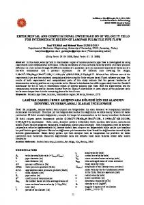
(2.2)
Figure 2.10 presents shape of this temperature distribution from Equation (2.2) for several values of ml. Maximum temperature always occurs at the center of the rod where
= .
Figure 2.10 Temperature distribution along a thin rod for several values of ml.
34
Several simplifications were assumed for the above analysis including constant heat transfer coefficient on the bridge surface, uniform cross section, neglecting the substrate under the bridge, and temperature independent electric resistance and therefore a uniform heat generation.
2.5.1 Lumped System Analysis
Figure 2.11 presents schematics of heat transfer components from the microbridge TCD. The heat loss to the surrounding gas,
, from the top of the bridge to the ambient
environment can be influenced by the gas flow velocity. We will show later that in absence of forced convection and operation in temperatures of few hundred degrees above ambient, effects of radiation and natural convection from a micro TCD is negligible [36], therefore conduction via gas medium is the dominant heat loss mechanism. Due to high aspect ratio of the micro bridge (order of 100:1), conduction along the bridge to the substrate, q3, is smaller. Also, given the substrates much larger thermal mass, its temperature is at almost ambient temperature even at locations close to the hot microbridge. This means conduction from below the microbridge, q2, is expected to be bigger than the top portion, q1, because of small gap between microbridge and the cool substrate. Overall major heat transfer from the bridge,
+
, is a function of thermal properties of the gas mixture. The small mass
microbridge is suspended in low thermal conductivity gases that makes it capable of reaching high temperatures at very low power levels of few microwatts.
35
Figure 2.11: Schematics of heat dissipation from an electro thermal bridge
Even though the complex three-dimensional geometry of the microbridge makes it difficult to use existing analytical solutions, the relation between sensor response, gas properties, and the applied power can be described with a Lumped System Method [39]. Lumped System Method includes the assumption that temperature variations within an object can be neglected in thermal analysis whenever heat conduction within an object is much faster than heat transfer across the boundary of the object, especially in this case thermal conductivity of silicon microbridge is three orders of magnitude larger than that of the surrounding gas medium. As this is a high aspect ratio microbridge (100:1), the significant amount of heat is conducted from its surface to the gas. By looking at the radial heat transfer and considering an average temperature for the microbridge, spacial temperature variations within the solid object is neglected for this thermal analysis, while nonetheless the average temperature of the microbridge used for Lumped analysis can still be variable with time.
36
Biot number gives an index of the ratio of heat transfer resistance inside and at the surface of a body. The Biot number is an indication of the applicability of Lumped System Method and is defined by Equation (2.3) ≡ Assuming
=ℎ
⁄
ℎ
(2.3)
≈ 1 which is true for conduction dominant heat transfer, then
h can be estimated as
ℎ≈
therefore, for this problem, Bi number can be estimated from Equation (2.4)
= In radial direction,
∙
(2.4)
can be considered the thickness of the bridge that is 1 µm, also
we assume that the characteristic length for conduction in gas medium is the gap under the microbridge i.e. 10 µm, therefor values for air 0.024
⁄ .
⁄
≈ 0.1. Substituting the thermal conductivity
and silicon 149
⁄ . , Bi number is estimated to be
≈
1.6 × 10 . Such a small Bi number verifies assumption of a lumped system and suggests a uniform temperature profile across the thickness of microbridge . At steady state, consideration of the energy balance implies that the rate of heat transfer from a lumped solid object is equal to the rate of heat generation within the object. For a high aspect ratio microbridge it can be written as
=
37
Where
is rate of heat generation in the microbridge,
is thermal conductivity of
surrounding fluid, A is surface area of the bridge and
is temperature gradient of
gas medium at external surface of the bridge that can be estimated using temperature of solid, ambient temperature
and a characteristic length of conduction, L, as
=
( −
≈
)
(2.5)
The left hand side of the above equation is dissipated electrical power, thus ( −
=
)
(2.6)
Where I is the electric current and R is the resistance. For a doped silicon, temperature dependence of resistance can be described with a linear model as = Where
(1 +
−
)
(2.7)
is the resistance of the conductor at reference temperature
resistivity temperature coefficient. For easier analysis, lets choose
and =
is and
substitute R in Equation (2.6) from Equation (2.7), thus (1 + ( −
)) =
( −
)
(2.8)
As equation (2.8) describes, temperature, therefore resistance, of the microbridge sensor at steady-state operation is related to thermal conductivity of gas medium at an input power. Left side of the equation describes the electrical phenomena and first order dependency to
38
the temperature while right side is conduction heat loss and is proportional to average temperature of the microbridge. From this equation the temperature change in microbridge can be obtained as ( −
)=
1 −
Or 1 ( −
)
=
−
Therefore at steady state, inverse of the average temperature change of the microbridge is proportional to effective thermal conductivity of the surrounding gas.
2.6 Initial Testing
The packaged sensor was mounted on a custom built PCB terminal through which each microbridge can be individually addressed. The package was placed in a 100 ml glass container that has inlet and outlet ports for gas flow as shown in Figure 2.12. The sensor was then subjected to different gases using mass flow controllers (Alicat Inc.) and excited with at constant voltages. The schematic circuit for measuring the real time resistance of the sensor is shown in Figure 2.12.
39
(2.9)
Figure 2.12: (a) The mass flow controllers used for mixing and regulating the flow. (b) The sensor mounted in a glass container and exposed to controlled gas. (c) The schematic circuit for measuring the real time resistance of the sensor. Figure 2.13 illustrates close up of Cold and Hot resistant response signals from the sensor in pure nitrogen. Data in recorded at high sampling rate, it is possible to reduce the electric noise an order of magnitude by taking a real time moving average. A closer look at the signals show that both cold and hot resistant slightly drift due to ambient temperature variations. Taking the difference of the two signals and working with the resistance change can eliminate this issue as shown in Figure 2.13.
40
Figure 2.13: Close up of Cold and Hot resistant response signals from the sensor. Taking the resistant change can eliminate small drifts due to ambient temperature changes. A moving average of high sample rate data reduces the electric noise (horizontal axis represents the number of samples, recorded at 1 MS/s).
Figure 2.14 presents change in resistance of the microbridge in three different pure gases, at three driving voltages. Consistent with thermal analysis, the resistant change increase as more power is applied to the sensor, however that also means the operating temperature of the sensor is higher. Therefore although more power gives a stronger signal, to protect the sensor from damaging, it should not be pushed to the limit. For the same applied voltage and current helium shows smallest resistance change, that is because its thermal conductivity value is the highest and according to equation (2.9) this should lead to the smallest temperature raise. On the other hand carbon dioxide has a bigger response
41
compared to nitrogen. These contrasts will allow us to detect a fraction of one gas in another medium.
Figure 2.14: Change in resistance of the microbridge in three different pure gases, at driving voltages of 4, 4.5 and 5V applied to the sensor.
In the next step microsensor operation was tested in gas mixture. Both 50 µm and 100 µm were tested for percentages of helium in nitrogen. Figure 2.15 shows the results obtained at three different power levels. The slope of the signal versus concentration represents the sensitivity and it is increasing as the power is raised. Overall the longer 100 µm shows more efficient performance that is because most of the heat is dissipated the narrow center of the bridge where resistance is higher. In the following chapters, response of the sensors in more gas species and with different methods are studied.
42
Figure 2.15: 50 um long microbridge and 100 um long microbridge with narrower center part were subjected to variation of helium in nitrogen mixtures at three different power levels.
2.7 Summary
In this chapter design and fabrication of a novel microbridge sensor was described. The microbridge is made of 1 µm doped polysilicon layer passivated with 200 nm of silicon nitride thin film for protection. The bridge is suspended from substrate via a 10 µm silicon oxide layer. Each die containing several microbridges is packaged in DIP chip, each bridge can be excited and measured individually. Geometrical and electrical characterization of the sensor were conducted to obtained accurate dimension and specifications. An analytical thermal solution was studied that provides insight on the electro-thermal phenomena. At the sensors were tested in different pure gases and gas mixture. Response of the sensor at 43
three power level was studied. Results show that at the same power level the longer microbridge has a better sensitivity to concentration variations that is consistent with our thermal analysis as it provides a better thermal isolation.
44
CHAPTER 3:
COMPUTATIONAL MODELING OF ELECTRO-
THERMAL PHENOMENA; SENSOR SIMULATION
In CHAPTER 2: we developed a thermal analysis using analytical approach to provide better understanding of electro-thermal phenomena in the sensor. It proved useful in describing the relationships between material properties, power consumption and the sensor response. However the general descriptive picture that it provided is not enough when it comes to design or accurately predicting the sensor response. A full scale computer simulation is potentially a better tool in this regard as it allows more complexity to be involved in the problem. As described in the Background of the first chapter, very little has been done on simulating the operation thermal conductivity detectors. Previous works have been limited to simple geometries with many simplifications in temperature distribution or heat flux. In this chapter we develop a comprehensive model capable of coupling physics such as convective flow, heat transfer, electrical current and joule heating. It involves using a realistic three-dimensional geometry, with multilayer composite material and applying temperature depend gas properties. The steady state is considered in this chapter, however in the following chapters the model is further developed to include the transient state.
3.1 Fundamental Equations and Numerical Approach
45
When a voltage is applied to the sensor, the geometry of conductive doped polysilicon layer determines the electric current distribution and therefore distribution of local heat generation over the bridge. The resistivity polysilicon itself is a function of local temperatures. The resulting local joule heating is then dissipated through condition via solid and gas medium. Potentially free or forced convective currents or radiation may be involved that can enhance the heat transfer. To include these phenomena the governing equations in steady state includes continuity equation that in vector notation is stated as ∇∙
=0
momentum equation is ∙∇
= −∇p + μ∇
+
and finally energy equation in the form of ∙∇
= ∇
+∅
Heat transfer is conjugate phenomena and in solid parts this equation is reduced to ∇ where
+
=0
is the volumetric heat generation that has a non-zero value only in the electrically
conductive layer; doped polysilicon. However to have the local
values, electric current
equation must be solved. =
( )
where σ is the temperature dependent electrical conductivity tensor and current density defined as 46
is the electric
= Once electric equations are solved,
∙
can be calculated and plugged back into the heat
equation, however, the temperature dependency of resistance make the equation system Fully Coupled. Such complex system of equations were handled in COMSOL 4.4 environment that allows for multiphysics modeling. Equations were discretized with finite element method.
3.2 Geometry, Meshing and Boundary Conditions
Figure 3.1 shows an optical image of the sensor under microscope of a thin flat doubly clamped beam. There are two planes of symmetry for the physical phenomena in this problem, as indicated by the dashed lines. For simulation purpose this allows us to model a quarter of the microbridge and significantly reduce computational cost.
47
Figure 3.1. Two symmetry planes of the problem, dashed lines represent orientation of the planes.
A detailed geometry of the composite bridge, obtained from SEM images, was used in three dimensional reconstruction of the bridge as shown in Figure 3.2. A unique aspect of this simulation method is direct inclusion of gas medium. This eliminates needs for assumption of temperature distribution or heat flux in the heat transfer problem. The extent of the computational domain was adopted large enough so it can represent the infinite surroundings of the microbridge. As gradients are expected to be smaller in the gas due to smaller thermal conductivity, the domain includes more volume of the gas than the solids. One great advantage of such modeling is that the only required thermal boundary condition will be the constant ambient temperature
=
on the outer boundaries.
.
Figure 3.2. Composition of microbridge model, because of two plane symmetry in the problem and to save in computation, only a quarter of the microbridge is simulated. 48
Bridge and surrounding gas ambient shown in the insert. Different layers of materials are labeled.
The continuity and momentum equations are solved for the gas medium, the heat transfer equation is solved for the whole geometry, while the electrical current equation is solved only for doped polysilicon layer; The electrical insulation BC ( = 0 ) is prescribed on the side boundaries of the beam while the anchor was set as the ground and a constant electric current density ( =
) was imposed on the other end of the beam to match the constant
current applied in the experiments. Room temperature of 20 oC and 1 atm absolute pressure were assumed as initial conditions, these also serve as BCs for the most outer boundaries. A symmetry boundary condition was used for the two planes of symmetry for electrical, free convection and heat transfer equations. The composite three dimensional geometry makes tetrahedral mesh the best choice for this modeling as it provides the best flexibility while allows to keep the total number of grid points lower compared to other structures. As shown Figure 3.2 utilizing a gradient scheme in grid point size was necessary to be able to handle both great extends of the geometry and small dimension of the bridge. The mesh is fine around the microbridge (0.1 µm) to resolve sharp temperature gradient and the small geometry features, it becomes coarser continuously with a factor of about 1.1 where it approaches the outer boundaries. Simulations were carried out with around 300,000 grid points on 8 CPU cores; each simulation took a few hours to complete. It was verified that the mesh resolution is fine
49
enough by rerunning the repeated simulations with a double fine mesh and observing a change of less than 0.1% in the results.
3.3 Thermo-physical and Electric Properties
Doping of polysilicon was assumed to be uniform. Resistance of doped polysilicon varies linearly with temperature and was implemented in the model according as = where
(1 +
is electric resistance at temperature
temperature
and
− ,
) is the base resistance at reference
is resistivity temperature coefficient.
and
for modeling are
obtained from electrical calibration of the fabricated sensors as described in Chapter 2. Thermal conductivity is another important property affecting heat transfer. In real world properties of gases varies considerably with temperature. This dependency cannot be considered in analytical approaches that is part of the reason those approaches fall short on accuracy. In our computational model however material properties are implemented as temperature dependent. Figure 3.3 shows Thermal conductivity and thermal capacity of the selected gases as a function of temperature, data was compiled from NIST database and was used in our modeling.
50
Figure 3.3 Thermal conductivity and thermal capacity of the selected gases as a function of temperature, data compiled from NIST database and was used in the computational model.
Moreover gas density, heat capacity at constant pressure, and dynamic viscosity are considered temperature dependent. Properties of solid materials were considered homogeneous and isotropic. For heat radiation calculations solid surfaces are considered
51
diffuse gray. The surface emissivity was set to 0.4 for silicon and 0.8 for silicon nitride, gas was considered a non-participating medium i.e. no volume radiation absorption.
3.4 Investigating Effect of Free Convection and Radiation
Potentially all three modes of heat transfer including conduction, convection and radiation can contribute to dissipation of heat from the microbridge. Even though the fabricated sensor is tested in stationary fluid, the effects of natural convection and radiation need to be investigated. For this purpose, a conjugate heat transfer model including non-isothermal flow and radiation from participating surfaces was implemented in COMSOL. A simulation was run with nitrogen as the gas medium and using an applied voltage of 5 V over the sensor. Figure 3.4a shows the obtained velocity streamlines of the free convection, colored with the magnitude of velocity. As heat is generated in the microbridge, it heats up the gas above it and the resulting buoyancy force cause a convective flow from the sides towards the region above the microbridge, with speeds reaching 80µm/s. Heat also radiates from microbridge surfaces towards the etched substrate and the surroundings. Figure 3.4B presents the radiative heat flux values on the participating solid surfaces, the highest radiative heat transfer rate at the center of the bridge is 2.5×10⁴ W/m2 while the conduction heat flux through the gas to the substrate was obtained to be of the order108 W/m2.
52
Figure 3.4: Modeling results of free convection and radiation over the microbridge in nitrogen with 5 V potential on sensor, (A) velocity streamlines colored with the magnitude of the velocity, (B) values of radiative heat flux on the microbridge and substrate surface
53
The average temperature on the surface of microbridge for this case was 636 K, using this quantity the Rayleigh number
was calculated. The Rayleigh number is a measure of
convective heat transfer strength, and is defined as (
= where gravity,
−
(3.1)
)
is the characteristic length i.e. length of the microbridge, is ambient temperature and
surface temperature of microbridge, deffusivity and
is acceleration due to
is surface temperature, in this case average is kinematic viscosity of the gas,
is thermal
is thermal expansion coefficient of gas. All the gas properties are
evaluated at film temperature
where
=(
+
)⁄2 . For pure nitrogen as the
surrounding gas and 5 V applied potential across the sensor,
= 5.56 × 10 . The
Rayleigh number is very small and confirms that the conduction is the dominant heat transfer mechanism for the problem. By comparing the results of simulations with and without radiation and convection, it was observed that convection and radiation are responsible for less than 0.1% of resistance change of the microbridge. For the radiation and convection heat transfer to be significant component, i.e. the order of few percent of the total heat loss, the temperature of the bridge would need to reach much higher values. Hence, subsequent simulations were carried out without convection and radiation, just examining the heat conduction through the gas surrounding the microbridge. This eliminates the need to solve for the flow field and saves significantly in computational costs.
54
3.5 Temperature Distribution and Resistance Prediction
Figure 3.5 shows the calculated temperature distribution on the microbridge surface as well as in the surrounding gas under in the presence of nitrogen. While dissipation of heat to the gas caused a small temperature gradient in the gas above it, temperature of the gas in the gap changes sharply. This is because the temperature of the substrate surface below the gap is within 1% of the ambient temperature due to the high thermal conductivity of silicon. Having such a low temperature within 10 micrometers of the microbridge causes a big portion of the heat to be dissipated below the microbridge, making the role of the thermal conductivity of the gas dominant compared to the other effects.
Figure 3.5: Temperature distribution from simulation in presence of pure nitrogen with an applied voltage of 5 volts (A) on surfaces of the microbridge (B) in surrounding gas and substrate
55
Figure 3.6 shows a plot of the calculated temperature distribution for three different applied voltages. Temperature at the anchor of the bridge is close to ambient temperature, while it is increasing farther away from this point; temperature at the center of the bridge is highest, this is because the center point is the farthest from highly thermally conductive solid substrate. At this point temperature was raised by about 500 K more than ambient temperature, for 5 volts potential. At higher voltages temperature of the mid-point could reach a critical value and the microbridge can start to burn-out. Experimentally, burn-out was typically observed for applied voltages in excess of 8V. 890 3V
Temperature (K)
790
4V
690
5V
590 490 390 290 0
5 10 15 20 25 30 Distance from the microbridge anchor (µm)
Figure 3.6. Calculated temperature distribution along half of the microbridge in nitrogen under three applied voltages. Response of the sensor to pure individual gases was simulated; the sensors were exposed to pure gases including nitrogen, carbon dioxide and helium, with constant input voltage applied to the circuit interface. A comparison of the computational and experimental results for each of the three gases mentioned is given in Figure 3.7. Among the three gases, the 56
resistance change for carbon dioxide was the greatest, while that for helium was the least. Simulation was able to predict change in resistance of the sensor within eight percent of error from experimental data.
Figure 3.7 Comparison of simulation and experimental results for sensor resistance change at three different operating voltages: 4, 4.5, and 5 volt pulses for three different pure gases.
Error! Reference source not found. shows the modeling results for how temperature and resistance of the microbridge change for three different gases at the same 5 volts potential; a change in the mean temperature of the polysilicon bridge alters its resistance and provide a tool to detect the surrounding gas. Overall, applying higher voltages (i.e. currents) yielded higher resistance changes for all three gases that were tested. Therefore, the sensitivity of the sensor increases with increasing operating voltages. At higher voltages the sensor reaches a higher temperature and is therefore more sensitive to the heat loss mechanisms
57
through the gas, although the sensor may be less stable at the higher temperatures when more power is consumed. . Table 3.1: Modeling results for power consumption, mean temperature, maximum temperature and change in resistance of the microbridge with 5 volts DC, for different gasses
Gas Composition
Power (mW)
Mean T (K)
Maximum T (K)
He N2 CO2
9.44 8.55 8.46
468 647 668
522 789 820
Resistance (Ω) 265 541 573
change
3.6 Simulation of Thermal Stresses
Our simulation results show that during the operation microbridge heats up to a few hundred degree C. This potentially can lead to considerable thermal stress. Previous works have shown correlations between stress in MEMS structures with reliability and life time of the devices [40-42]. In this section we add a mechanical analysis to the existing model to investigate levels and locations of thermal stresses in the hot sensor. The governing linear elasticity equations which are partially coupled with the heat transfer equation, are the equation of motion
58
Strain-displacement equation
and constitutive equation for isotropic homogenous media
where ν is Poisson's ratio and E is Young's modulus, σ represents the stress tensor, ε is the strain tensor and u is displacement. A material is said to start yielding when its von Mises stress reaches a critical value known as the yield strength. von Mises stress is defined as
where
,
,
are normal stresses and τ is the shear stress. Figure 3.8 shows
distribution of von Mises stress on the microbridge in typical steady-state operational condition in nitrogen at 4 mW. Due to mismatch of thermal expansion coefficient between silicon nitride and polysilicon a considerable tension stress is developed in the silicon nitride layer around the center of the bridge. The vertical displacement due of the bridge due to these thermal stresses is shown in Figure 3.8c and is less than 10 nm.
59
Figure 3.8: (a) and (b) Von Mises Stress along the microbridge, (C) distribution of the vertical displacement, under steady-state power of 4 mW.
3.7 Suggestion for Improved Efficiency
The insights provided by our analytical approach and thermal simulations can serve as a tool to suggest improvements for the future designs. One major goal in many applications is to obtain a stronger signal for lower consumed power, in other words, achieving a better power efficiency. Solid constituents have relatively high thermal conductivity and our results so far show that conduction along the beam and more importantly conduction through the gap underneath the sensor have important role in heat transfer while solid
60
pathways of heat don’t contribute to gas sensing. From this aspect it will further improve the efficiency if design provide more thermal isolation for the heated element. It was observed that temperature distribution on the microbridge was non-uniform with its maximum occurring happening at the center. As there are higher limits for the temperature, it means the whole temperature distribution is limited by the maximum values. From this aspect it will be beneficial if the temperature distribution can be more uniform over the heater, although a fully uniform distribution cannot be achieved because of conduction in solid material. To improve the above issues, we suggest optimizations to the beam anchor region while keeping all strong aspects of the current technology such as small dimensions, low power consumption, great surface to volume ratio and high aspect ratio. The recommendation includes having wider anchors made out of same electrically conductive material as the microbridge center, and suspended from the substrate as shown in Figure 3.9. The idea is that this wider part will have several folds less electrical resistance than the thin bridge due to the larger cross section. Therefor it provides electrical connection while doesn’t contribute to the power consumption; almost all the heat will be dissipated on the thin microbridge. The thermal resistant of the solid structure in this design is much higher the wider anchor are suspended from substrate and don’t participate in heating. Thus a larger portion of heat will transfer through gas medium. To improve the thermal insulation further, it will be beneficial to increase the gap size. However it will be too costly to increase the thickness of the current silicon oxide sacrificial layer to more than 10 µm size. To achieve a larger gap height, silicon nitride layer can be
61
deposited directly on silicon substrate and then the silicon substrate can be etched to create cavities of a few hundred micrometers.
Figure 3.9 A thermally optimized design with wide anchors. Also the bridge can be made wider (e.g. 5 µm) and thinner, this will keep the total resistance and surface area of the bridge almost same while eliminates need for electron beam lithography. This design is especially more convenient in applications where a metal thin film is used as the heater. The new design was simulated in nitrogen with the same model and conditions that was described in this chapter. Figure 3.10 shows the temperature distribution on the heated structure (a), and in the gas medium around the bridge (b). Temperature profile is more symmetric in the gas above and below the bridge that make it more independent of the gap size. Figure 3.10c presents the power density distribution and verifies that the triangulate anchors don’t participate in heat generation. Figure 3.10d is the temperature profile on the center line of the bridge with a flat center.
62
Figure 3.10: Simulation of the wide anchor bridge in nitrogen at 4 mW (a) temperature distribution on microbridge surface, (b) symmetric temperature distribution in the gas ambient, (c) heat dissipation density, (d) temperature profile at the centerline.
63
3.8 Summary
In this chapter a novel computational model was developed, that is capable of predicting the microTCD response, and revealing the local temperature distribution. The model utilizes realistic three dimensional geometry and minimal simplifications. It directly solves for temperature in both solid and gas surroundings by coupling momentum, energy and electric current equations. Results showed a highly non-uniform temperature distribution on the sensor, with maximum temperature value and location, and heat fluxes. Effect of natural convection and radiation was modeled and it was shown to be small. Thermal stresses were calculated and locations of maximum stresses were identified. Results show that the stress can put a limit to the operational power as well as temperature. The model was prepared with minimal simplifications; it includes the joule heating of doped polysilicon with temperature dependent resistance, considers temperature dependent properties for the surrounding gas, and is capable of modeling radiation and convective heat transfer as well. Simulation calculates the temperature distribution in the microbridge and provides electrical resistance of the sensor. The simulation platform developed in this chapter provides a great tool for future designs and optimizations in this field.
64
CHAPTER 4:
TRANSIENT ANALYSIS OF MICRO-ELECTRO-
THERMAL SENSOR; A NOVEL METHOD OF DETECTION
4.1 Introduction
During the past few decades, gas sensors, detectors and analyzers have been widely used to measure the composition of gas mixtures or to detect the presence of particular species in a gas medium.[2] Despite advancements in fabrication of micro sensors and efforts on pushing the dimensions to smaller limits, methods of measurement for using those sensors are still underdeveloped; the main method in real applications remains to be based on steady state readings from a conventional Wheatstone bridge. [12] [13] [14] [15] A micro thermal conductivity gas sensor, unlike calorimetric or metal oxide gas sensors, is based on changes in the thermo-physical properties of surrounding gas and do not rely on gas adsorption and reaction with a catalyst or thin films. Therefore, the response speed is more rapid, and the sensor can be operated in a continuous manner and be repeatedly used without memory effects due to absorption/desorption reactions. This property opens up great potentials for utilization of faster and more robust measurement techniques. The frequency methods and time domain thermo-reflectance (TDTR) are a few example of non-steady state methods that have been used in other applications for measuring thermal conductivity of solids specimen. Also Transient hot wires (THW) have been utilized in measuring properties of some fluid samples [24, 25]. Relatively large geometry of detectors
65
used in these studies involved long settling times, losses, complex 3D isotherms, natural convection effects and radiation. While our results so far showed correlations between steady state temperature and response of the sensor with gas composition, characteristics of a transient response may provide a similar or better accuracy within smaller time or utilizing less power. Especially ultra-small dimensions and therefore low thermal mass of our developed microbridge makes it a good candidate for this study. In this chapter, we develop a new measurement method, test bed, and experiments for optimum operation of the sensor in gas mixtures. To provide more insight and anticipate microsensor behavior, an accurate multiphysics model is developed that is capable of simulating transient response of the sensor in a gas medium without major simplifications. The developed technology is especially suitable for emerging ultra-portable and wireless gas analyzers in the “Internet of Things” era, where power consumption and footprint are critical criteria.
4.2 Thermal Analysis of Micro-Electro-Thermal Gas Sensor; Analytical Approach
So far thermal analysis have proven to be useful in understanding of sensors operations in other applications such as flow speed sensors.[20] Electro-thermal gas sensors work based upon the interaction between heat generation in an electrically conductive suspended element, and heat transfer from the element via the surrounding gas medium. We 66
introduced a sophisticated thermal analysis for steady-state response of the microbridge sensor in CHAPTER 2:. To further understand sensor performance in transient regime, we extend the thermal analysis to include a full transient solution. Figure 4.1 presents schematics of heat transfer components from the microbridge TCD. The heat loss to the surrounding gas,
, from the top of the bridge to the ambient
environment can be influenced by the gas flow velocity. Previously we showed that in absence of forced convection and operation in temperatures of few hundred degrees above ambient, effects of radiation and natural convection from a micro TCD is negligible [36], therefore conduction via gas medium is the dominant heat loss mechanism. Due to high aspect ratio of the micro bridge (order of 100:1), conduction along the bridge to the substrate, q3, is smaller. Also, given the substrates much larger thermal mass, its temperature is at almost ambient temperature even at locations close to the hot microbridge. This means conduction from below the microbridge, q2, is expected to be bigger than the top portion, q1, because of small gap between microbridge and the cool substrate. Overall major heat transfer from the bridge,
+
, is a function of thermal properties of the gas
mixture. The small mass microbridge is suspended in low thermal conductivity gases that makes it capable of reaching high temperatures at very low power levels of few microwatts.
67
Figure 4.1 Schematic of heat dissipation from an electro thermal bridge
Considering the geometry and dimensions of the problem Bi number estimation remains ≈ 8 × 10 . Such a small Bi number suggests that a
same as steady-state situation,
lumped system analysis can provide insights for both steady state and transient thermal phenomena. At steady-state, we concluded that the average temperature change of the microbridge is inversely proportional to effective thermal conductivity of the surrounding gas as 1 ( −
)
=
−
At transient state, i.e. the moments when sensor is switched on or off, microbridge temperature varies between
and the hot operating temperature, and changes
proportionally to the heat capacity of the microbridge. By adding a transient term, energy balance equation is extended to
=
+
68
(4.1)
It implies that the rate of heat generation within a lumped solid object is equal to sum of the rate of heat transfer from the object and rate of energy storage within the object. Where is rate of heat generation in the microbridge, where ρ is the density of the microbridge which is the dominant thermal mass in the system,
is thermal conductivity of
surrounding fluid, A is surface area of the bridge and
is temperature gradient of
gas medium at external surface of the bridge that can be estimated using temperature of solid, ambient temperature
and a characteristic length of conduction, L, as
≈
( −
)
(4.2)
The left hand side of the above equation is dissipated electrical power, thus
=
( −
+
)
(4.3)
Where I is the electric current and R is the resistance. The same verified linear model is used for temperature variations of doped silicon resistance, that means = Where
(1 +
−
)
(4.4)
is the resistance of the conductor at reference temperature
resistivity temperature coefficient. For easier analysis, lets choose
and =
is and
substitute R in Equation (4.3) from Equation (4.4), thus
(1 + ( −
)) =
+
69
( −
)
(4.5)
Unlike steady-state case, power generation (the right hand side of the above equation) isn’t constant as temperature is varying even though a constant current is applied. In absence of heat generation, when cooling happens, this equation is reduced to the following form ( −
=−
)
where T is the average temperature of the bridge,
(4.6)
is the ambient temperature, t is time.
This, in fact, states Newton's Law of Cooling, where the rate of heat transfer from a cooling object is proportional to the temperature difference between the object and ambient. Such a differential equation has a solution with exponential form of
( )
Where
=
⁄
=
+(
)
−
(4.7)
is the time constant of the exponential transition.
When electric current is applied and the bridge is heating up to the operating temperature, Equation (4.5) can be rearranged as −
+
( −
)−
=0
And furthermore
+
1
−
+
− 70
=0
Solution to this equation is similar to the cooling case and time resolved temperature equation is obtained as
−
=
1−
−
(4.8)
Where the time constant τ for the heating case is defined as
=
−
(4.9)
This analysis shows that the time constant of the heating is inversely proportional to the gas mixture thermal conductivity and the input power 1
−
=
(4.10)
This analysis shows that the time constant of the heating is inversely proportional to the gas mixture thermal conductivity and the input power. The term
represent the total
thermal capacitance of the system. kf is the effective thermal conductivity of the gas medium which is responsible for most of heat lost from the bridge. A portion of heat is conducted along the bridge to the solid substrate, in which case, thermal conductivity of solid, ks, plays a role. 71
4.3 Developing a Thermal Resistance Circuit:
There is an electrical analogy with heat transfer that can be exploited in problem solving and could help in understanding the system and effect of each parameter. The analog of heat transfer rate
is current, and the analog of the temperature difference,
voltage difference. From this perspective a heat transfer resistance
, is
can be defined as
−
=
−
(4.11)
For heat conduction through a medium, thermal resistant is obtained as
= ⁄( ∙ ). The
thermal resistance increases as L increases, as A decreases, and as k decreases. Once heat is generated in the polysilicon core, it transfers either to surrounding air or along the bridge to the substrate that rests at ambient temperature. These two thermal resistors act in parallel and are indicated in Figure 4.2 with
⁄(
For this situation, the total heat flow
is made up of the heat flow in the two parallel paths,
∙
) and
⁄(
∙
)
with the total resistance given by 1
=
1
+
1
=
∙
+
∙
For the thermal circuit to be able to describe the transient state, thermal capacitors should be taken into the account too; in analogy with electric circuits, thermal capacitance can be defined as 72
=
and consists of two parts; thermal mass of the solid material, gas medium,
(4.12)
=
, and thermal mass of
. However it is estimated that thermal mass of the solid bridge is
considerably larger than that of its surrounding gas.
Figure 4.2 The thermal circuit developed for the microbridge sensor; subscript “s” indicates solid material properties and “g” corresponds to surrounding gas properties.
Heat generation can be modeled as a current source with total power of
sent into the
circuit. A switch can simulates the moments that thermal excitation starts or stops; when a current pulse is sent to the sensor, it is equivalent to closing the switch in the thermal circuit. Part of the heat flows through parallel resistors and part of the heat is stored in the parallel capacitors as internal energy. Once capacitors reach steady state temperature (equivalent to steady voltage in the circuit), all the heat flows through the resistors and capacitors act as open circuit (steady-state). When excitation pulse ends, it is same as opening the switch 73
in Figure 4.2; in this case the source is out and the energy stored in capacitors is discharged through the thermal resistors until all temperatures reach ambient T. This provides insight on how properties of solid and gas material can affect the sensor response. The analytical approach discussed in this section provides insights on dependency of the sensor temperature (i.e. resistance) to the gas medium properties and verifies that the time constant of transient heating or cooling can provide data on thermal conductivity of the gas. However analytical models involve many simplifications and fall short in taking real word application details into consideration or in providing accurate numbers that can be used for design. For this reason computer simulation and experimental results are required on the path to develop and evaluate the new sensors and methods of measurements.
4.4 Experimental Technique and Materials
Low power and rapid response of our recently developed sensor make it suitable for a fast time resolved response study. A variation of our polysilicon microbridge was selected for the experiments that is 100 µm long and has a 1 × 1 µm cross section doped polysilicon layer, suspended through a silicon dioxide sacrificial layer. The other mass on the bridge is a 200 nm silicon nitride passivation layer, meant to provide electrical isolation and protect the bridge against any reactions at high temperatures. Half of this microbridge at its center is made narrower to keep more of the resistance and therefore the generated heat at the center, farther from solid anchors.
74
As mentioned earlier, doped polysilicon resistance changes highly with temperature, the average temperature of the bridge can be correlated to its resistance. Electrical characterization of the sensor was carried out to determine base resistance
and
Temperature Coefficient of Resistance, , for modeling and experiments. The sensor was placed in a temperature controlled oven and was subjected to a series of uniform steady temperatures up to 80 ˚C. For the microbridge in this study, a TCR of and a base resistance of
= 0.0013 1⁄℃
= 3084 Ω at 23 ˚C were measured.
For experimental studies, a flow system was designed, capable of subjecting the sensor to targeted accurate concentrations of gas mixtures. Ambient air is composed of 79% nitrogen and its thermo-physical properties is very similar to nitrogen. Therefore nitrogen was selected as the carrier gas for our experiments in controlled lab conditions. Each specific target concentration of an analyte was achieved by mixing the flow from a bottle of premixed 5% analyte in nitrogen, and the flow from a pure nitrogen bottle, as shown in Figure 4.3. By adjusting the flows through two high accuracy Mass Flow Controllers (Alicat Scientific Inc. MC series) analyte concentration can be controlled between 0% to 5%. The sensor was installed in a 100 ml small glass container connected to gas flow tubing, and was placed inside an insulated oven to provide temperature stability and eliminate room temperature fluctuations. The sensor container was flushed with the desired gas mixture for each measurement and a total volumetric flow of 500 standard cubic centimeters per minute (sccm) was maintained during data collection to ensure mixture of gas doesn’t change over time. Large enough size of the container and proper location of
75
the sensor in it, made convection effects negligible at this flow rate. Mixtures of helium, methane, carbon dioxide, and argon, in nitrogen were tested.
Figure 4.3 Diagram of experimental setup including the flow control system, data acquisition devices and circuit interface and signal processing unit.
16-bit analog to digital and digital to analog converters (National Instrument PCIe-6351) at a high sampling rate of 1 MS/s was employed for data acquisition. Such high sampling rate is essential to be able to resolve the fast transient variations. Serving as interface 76
between PC and rest of experimental setup, it is capable of generating waveforms for pulsed excitation of the sensor while simultaneously reading the analog output from measurement system. The excitation waveform is generated at a higher 2 MS/s. A circuit interface was designed that can apply a constant current across the sensor and translate sensor resistance into an output voltage, measureable by the data acquisition card. Conventionally, Wheatstone bridge is utilized to generate an output signal for such MEMS sensors, however a Wheatstone bridge cannot keep neither current nor voltage constant over the sensor, therefore expresses nonlinear output at extended range of measurements. Figure 4.3 includes schematic of the developed circuit interface consist of a reference resistor (4 kΩ), two other auxiliary resistors (300 Ω each) and an Op-amp. Upon application of an input voltage,
, the current I passes through the branch that includes the
reference resistance. The Op-amp keeps the voltage of its inverting and non-inverting inputs equal by changing the output voltage,
, this pulls a constant current through the
sensor equal to the current passing through the reference resistor. Therefore resistance of the sensor
at any instance can be obtained from equation (4.10). As long as
is
maintained constant, the current passing through the sensor will be constant regardless of its resistance variations. − +
=
(4.13)
To improve precision and stability under normal room temperature fluctuations, resistors are selected to have small temperature coefficients of less than 20
77
⁄ ℃.
Initially OP177 (Analog Devices Inc.) was selected as the Op-amp for the interface, because it offers low noise and ultra-low offset voltage of 25 µV and a offset voltage drift of 0.3 µV/˚C. However initial experiments revealed that Slew Rate of 0.3 V/µs wasn’t fast enough to resolve the sensor fast response. Slew rate is the maximum voltage change per unit time that an amplifier can generate on its output. Therefore it was changed to LT1028 (Linear Inc.) that offers a Slew rate of 11 V/µs at the cost of slightly higher noise level and higher offset voltage drift of 1 µV/˚C. The small output offset of 15 µV on this model can be adjusted to zero through an added trimmer resistor. More details about the specifications of the chips can be found in Appendix B. When no electric current is applied, microbridge is at ambient temperature and its resistance is minimum; we called this cold state and its corresponding resistance is referred to as base resistance or cold resistance,
. The excitation pulse is designed such that circuit
can also measure the base resistance by applying about 100 µA current and reading hot operation,
. At
switches to a predefined high value and microbridge temperature,
therefore its resistance, increases; this state and the corresponding resistance are referred to as hot state and hot resistance in this study. In previous Chapter 2 we showed that this value can change further depending on composition of the ambient surrounding gas. Passing a DC current, continuously operates the sensor at hot temperature and generates the steady-state output signal. However to study the sensor transient response regime, we excite the sensor with square current pulses. Transient variations occur upon each rising or falling edge. As side benefits, pulsed excitation can save in energy to few fold and eliminates heating of the chip and slow resistance drifts over time.
78
Figure 4.4 shows an input pulse train for
and the corresponding calculated resistance of
the sensor in nitrogen. Circuit interface turns the voltage pulse to a current pulse according to equation (4.10). Thanks to the very low thermal mass and fast response of the microbridge, in less than 2 ms it reaches steady state hot temperature and can provides one set of measurement. To make the next measurement, enough time should be allowed for sensor to cool off. Experiments showed that a 50 Hz pulse with duty cycle of 10% can prevent the drift while providing 50 measurements per second. This is fast enough even for applications such as Gas Chromatography. As shown in Figure 4.4, the low voltage in the pulse train was set to 0.25 V; it runs a current about 80 µA across the microbridge and makes it possible to measure cold resistance from
79
.
Figure 4.4: Input pulse train, corresponding output voltage and calculated microbridge resistance for a duty cycle of 10% applied.
In applications where chemical composition of gas medium does not vary quickly, i.e. stable over a second such as in our experiments, taking a moving average on readings can
80
improve the accuracy of measurements and cancel noise from electronic sources. While hot resistance values provide the sensor response, monitoring cold resistance can show variations of ambient temperature and could be used to compensate for the corresponding change in resistance.
4.5 Simulation of Transient Phenomena in Microbridge
Although, based on our extensive literature review, little work has been conducted on developing computer models for thermal sensors, [13] [21] [11] there was almost no efforts on transient modeling of these sensors. One reason could be the lack of transient detection methods for practical applications. However with our newly developed technique, it is highly useful to have a transient computational model capable of anticipating the sensor response and performance. Such a model could be used in optimization of design parameters. In this chapter our previous comprehensive model that was described in Chapter 3 is further developed to include the transient phenomena [43, 44]. The advantages of the current simulation model remains to be utilizing the realistic three dimensional geometry, minimal simplifications, including the mutiphysics phenomena including electrical and heat transfer, and temperature dependent material properties. For this purpose the governing equations have to be solved that includes the transient terms. As in the following vector notation continuity equation will be
81
+∇∙
=0
then momentum equation is stated as
+
∙∇
= −∇p + μ∇
+
and finally energy equation in the form of +
∙∇
= ∇
+∅
The governing equations along with electric current equation in the conductive polysilicon are discretized with finite element method in COMSOL 4.4. Information obtained from microscopy and SEM images were used towards three dimensional reconstruction of the bridge. The model was meshed with 500,000 tetrahedral gridpoints that are fine, about 0.04 µm, on the bridge and smoothly get larger close to the outer boundaries where gradients are negligible. Modeling the realistic geometry requires a heavy mesh and therefore an efficient meshing of the space is important, this gets even more critical as transient simulation takes up 100 times more computational cost as all the equations must be solved for very time step. Both solid materials and surrounding gas are included therefore no assumption and simplification was employed for thermal interaction of the gas and solid interface. However free convection and radiations are neglected as in previous chapter we showed that their effect is very small. The computational domain is large and extended at least 200 µm from the bridge in each direction. 82
The only thermal condition required on the domain outer boundaries is constant room temperature. As a wide range of temperatures are involved, properties of solids and gas are considered temperature dependent and taken into account for further accuracy. Electrical and heat transfer physics are coupled in the model. The input current and ground voltage are provided as a boundary condition to the ends of the microbridge. The model handles heat generation, heat transfer, and resistance calculations. The equations are also discretized in time; from cold state to the hot temperature for this sensor, about 300 µs of time is required. This time domain is divided into 100 time steps. As computational cost of these simulations are high, an efficient exponential scheme was applied that adjusts the time step to the rate of changes; from the thermal analysis we expect that the temperatures increase in an exponential manner, as shown in Figure 4.5 the time step size is adjusted based on these variations. Compared to conventional equal time steps this can reduce the number required time steps over two times and results in better time resolution close to the initial conditions where rate of changes are higher. On the other hand time steps are larger close to the steady state.
83
Figure 4.5: The adaptive time step division applied for simulations compared to conventional equal time steps. For the same number of steps adaptive scheme results in better time resolution close to initial condition where rate of changes are higher.
All temperatures are set to the room temperature as initial condition. Initial power of the sensor is set to zero, however electrical boundary condition will force the power to jump up to the operational power upon simulation starts running. Under the imposed conditions it takes several hours for each transient simulation to complete. Figure 4.6 shows evolution of temperature distribution developing over the sensor and the surroundings from initial condition (t = 0 s) to steady state (t = 300 µs) at 2 mW.
84
Figure 4.6: Simulated temporal evolution of temperature distribution in the microbridge and the gas medium nitrogen under 2 mW, from initial condition (t=0 s) to the steady state (t=300 us) a quarter of the geometry is shown.
4.6 Comparison of Time Resolved Results Figure 4.7 presents a close look at resistance change of the microbridge in nitrogen, in response to a square current pulse of 0.7 mA and 2 ms width. The first few hundred microseconds of the response corresponds to the transient heating due to thermal mass of the micro sensor; this part is ignored for the conventional steady state measurement. In the 85
second millisecond of hot operation, temperature field is already fully developed and resistance has reached its steady state. In this work we studied both transient and steady state regimes for comparison.
Figure 4.7: A close up of an input pulse and the resulting sensor signal in pure nitrogen. Steady-state and transient regions corresponding to heating and cooling are clearly distinguishable at this time scale.
According to our thermal analysis in previous section, it is expected that the microbridge resistance, i.e. its average temperature, responds exponentially during a heating as Equation (4.14) 86
=
where
is base resistance,
+(
−
)
(4.14)
is hot resistance, t is time and τ is the time constant of
transient signal, i.e. time required to achieve 63.2% of the total resistance change. As shown in Figure 4.8, τ was obtained from experimental and simulation results by fitting an exponential curve using least square method
Figure 4.8 Extracted heating curves from experiment and simulation results at 2 mW, and the fitted curve. A time constant of 65 µs was obtained for this case.
Figure 4.9 presents steady state and transient microbridge response in pure nitrogen at three different power level
, where I is the high current value corresponding to the square
excitation pulse train. As expected from our heat transfer analysis, 1⁄ varies linearly with power while 1⁄∆ has an inverse relation with power. Both resistance change and τ are increased at higher powers and therefore can provide a better sensitivity at higher powers. 87
However for currents over 1 mA this sensor shows instabilities due to very high local temperatures, thus in practice there is a higher limit to the input power. The trend of data coincide with thermal analysis that and suggests that at the lower end, as power approaches zero, ∆
approaches zero too while τ is approaching a constant value. Equation (4.9)
anticipates that this value is equal to the time constant of the cooling phenomena.
Figure 4.9: Experimental and simulation data for (a) steady-state resistance change and (b) transient time constant, at three different power levels.
88
Further experiments were conducted with gas mixtures at the higher power level of 2 mW. Figure 4.10 shows how the sensor responded to change of concentrations. A square current pulse of 50 Hz with duty cycle of 10% (2 ms width) excited the microbridge. Transient time constant was extracted from the first 300 µs of output pulse, simultaneously, steadystate resistance changes were calculated from the last 1 ms of it. Results were averaged over the course of 30 seconds to reduce electrical noise. Having the smallest thermal conductivity among those tested, helium expresses the largest contrast with nitrogen carrier. Same linear behavior was observed for resistance values and time constant.
89
Figure 4.10: (a) steady-state and (b) transient response of the sensor to mixtures of nitrogen with helium, carbon dioxide, methane and argon. Analyte concentration was varied from 0 to 5%
Table 4.1 summarizes sensitivity and minimum level of detection for different gases in nitrogen. The values are calculated from data in Figure 4.10 and standard deviation of resistance and time constant of individual pulses, 0.015 Ω and 0.0022 µs respectively. The reproducibility of overall gas flow and sensing system through multiple experiments was 0.25 Ω for resistance and 0.035 µs for time constant. Table 4.1 Sensitivity and levels of detection for both steady state resistance change and transient time constant
For transient measurement purposes both heating and cooling curves could be used, however in this study we focused on the heating curve. Cooling curve provide less benefit as it first requires the microbridge to heat up to a steady operating temperature. Based upon our experimental results this takes over a millisecond, however when the heating curve is
90
used only 300 µs of data is needed, so that a shorter pulse duration can be utilized for the measurements. Therefore use of the cooling curve will a longer pulse duration, of several milliseconds, and hence more energy and time for each measurement. To make it easier to compare data with heat transfer analysis, power levels reported in the figures corresponds to the DC power of
, where I is the high current value
corresponding to the square excitation pulse train. Because a 50 Hz pulse train with 10% duty cycle was utilized in this method for sensor excitation, the actual power consumption for continuous measurement was maximum 200 nW (4 nJ per single measurement) that is the lowest reported power management on a TCD so far.
4.7 Summary
In this chapter a new method for measuring gas composition with thermal conductivity gas sensors was introduced, that is based on analysis of transient thermal response. The novel method was implemented and tested, for the first time, for detection of gas mixtures with a miniaturized microbridge heater. Our analytical approach in study of sensor transient thermal phenomena revealed that the system’s response to a current square pulse is exponential and that the time constant of this response could be correlated to the thermal conductivity of gas mixture. An experimental setup for precise controlling of gas mixtures flow was integrated to a fast data acquisition system to experimentally investigate detector response to change in mixtures of helium, carbon dioxide, argon and methane in nitrogen. An automated program 91
was developed that simultaneously excites the sensor and reads the system response to it and can resolve variations down to 1 µs. Very low thermal mass of the micro sensor results in ultra-fast respond of only 300 µs that allows for rapid scanning rate. The proposed method was experimentally compared with the conventional steady state resistance readings. Results show that with the same hardware, transient method provides similar or better sensitivity using a fewer number of samples. Moreover transient analysis eliminates need for waiting for the system to reach steady state and therefore is faster. Unlike ∆ , the time constant τ does not approach zero when power is reduced towards zero. Analysis show that instead it approaches a value that is close to the cooling time constant of the microbridge. Our sophisticated computational modeling of the sensor was further developed to include simulation of the transient thermal behavior of the sensor. Due to minimal simplifications, numerical results were in agreement with experiments in estimating the transient curve and time constant. This provides a powerful simulation tool that could be utilized in design of the future mico/nano sensor technology. Making efficient measurements is not only a result of pushing the microfabrication to the limit but also requires developing improved measurement methods and low noise circuitry. This method compared to the conventional methods offers a few fold reduction in power consumption without need for modifications in sensor. The low voltage, and low power required for this μTCD sensor measurement system allow it to be combined with ultra-portable, wearable sensors, and wireless technology for data
92
processing and communication. Evolving miniature gas analyzer technologies such as micro gas chromatography systems demand integration of highly efficient micro detectors.
93
CHAPTER 5:
3ω TECHNIQUE FOR MEASUREMENT OF GAS
CONCENTRATION IN A MIXTURE; THE AC EXCITATION METHOD 5.1 Introduction
During the past decades, more efficient measurement techniques for thermal conductivity have received growing attention due to the emergence of novel and challenging to measure materials, including thin-films, superlattices, biological samples, and nanomaterials.[26, 27] In these areas, enhanced thermal property information could aid a diverse range of applications, including improved microprocessor heat removal, higher efficiency thermoelectric materials, and more effective minimally invasive cryosurgery. [45, 46] Our steady-state DC measurements and impulse response time resolved measurement techniques were described and applied for detection of gases in the previous chapters.[36] One important class of measurement techniques for dynamic systems are methods based on AC thermal excitations. The main motivation in this method is to use a narrow-band frequency detection technique and therefore obtaining a relatively better signal-to-noise ratio.[47] Similar to our other techniques, here an element itself can serve as a heater and at the same time a temperature sensor, if it is electrically conductive and with a temperature-dependent electric resistance. Feeding an AC electric current of the sinusoidal form across a conductometric element creates a temperature fluctuation on it and accordingly a resistance fluctuation at second
94
harmonic. This further leads to a voltage fluctuation at the higher harmonics across the element. [48] Corbino [49] showed that the temperature fluctuation of an ac heated wire gives useful information about the thermal properties of the solid constituent material. More investigations of the AC method were carried out later[50] and mainly in the last couple of decades[51, 52], which made the method more practical. In theoretical approaches, the heat conduction equations that describes the method, was solved under the approximations either only for the high frequency limit,[53, 54] or only for the low frequency limit.[55] With those approximations one lost either the information on the thermal conductivity or the information on the specific heat of the specimen. Later an explicit solution for the one-dimensional heat-conduction equation was provided.[48] With this solution and by using a modern digital lock-in amplifier, it was made possible to obtain both the specific heat and the thermal conductivity of a rod- or filament-like specimen simultaneously. A different class of experiments involved joule heating a serpentine wire on a platform for measuring thermoelectric properties of nanostructures, that applied a large direct current and measuring the resulting temperature rise using lock-in detection of a small alternating current superposed through the same heater.[56] Dames et.al [48] combined the dc-heating with ac-detection in experiments for a line heater on the Pyrex substrate and developed a more general framework of thermal and electrical transfer functions. By means of a DC offset superposition, in this method lower first and second harmonics also contain information about thermal properties. This eliminates the
95
need for higher-harmonic detection and may also be useful for systems with very fast thermal response. So far the AC thermal excitation method has been used as a tool for measuring thermal conductivity of solid constituents, films and substrates, while fluid samples have typically been studied with traditional steady state methods. The challenge of implementing an AC excitation method for gas detection application is that the solid material of sensor typically has much larger thermal effusivity,
, than the gas surrounding it. The periodic heat
generation in the conductive heater will split between the solid substrate and the surrounding gas based on their ratio of thermal effusivities, that can have their values different by two orders of magnitude,[57] therefore much of the heat will enter the substrate rather than the gas. As a result, a significant part of the 3ω signal will come from the substrate, rather than the fluid under test, which decreases the signal of interest’s size. In this chapter we implement a custom 3-Omega AC measurement technique for our microbridge heater for the purpose of high accuracy, low power gas sensing. The sensor performance is evaluated for binary mixtures of CO2, Ar, He and CH4 in nitrogen for the first time. The customized experimental setup are developed including a 3-Omega circuit that controls the AC heating current and conditioning of the 3-Omega output voltage signal. The amplitude and phase lag, and the in-phase and out-of-phase components of the 3Omega signal are investigated for each case and are studied correlated to changing gas concentrations.
96
5.2 Mathematical Development of 3ω AC Method for Gas Sensing The AC excitation technique offers a new approach to gas sensing that is amenable for low power gas sensing applications. One unique aspect of this method is that it can potentially operate without individual sensor calibration unlike several other gas sensors. Previously, variations of this technique was pioneered to measure the thermal conductivity of thinfilms and was described in the literature[58]. Our AC detection method is based on operating the sensor at a narrow-band frequency; the micro-electro-thermal sensor is thermally excited with an electrical current of angular frequency ω = 2πf and root-mean-square value (RMS) Iω,RMS that is driven through the heater line. The resulting joule heating value is product of the current square by the sensor resistance, thus occurs at the frequency 2ω. =
=
=
.
.
(
)
)=
.
.
(
.
(2
1−
)
2
The periodic heating creates a thermal wave that penetrates the surrounding environment. The amplitude of the temperature oscillation at the source depends on the thermal properties of the environment. The periodic temperature oscillation follows the periodic heating and occurs at a frequency 2ω but delayed in phase φ (i.e., the phase lag). Such a relation may be described generally by a linear transfer function Z, where Z depends on properties of solid and gas materials ∆ =
⊗
,
97
∆ ∝
∆ =
.
.
.
(2 2
1−
+
)
(5.1)
The Temperature Coefficient of Resistance then causes the resistance of the heater to oscillate at 2ω as.
=
(1 + . ∆ ) =
+ .
.
1−
.
(2 2
+
)
(5.2)
The resulting voltage across the sensor, is the product of current, and resistance, therefore will have a component at 3 times the current frequency (3ω) stemming from product the 1ω current and 2ω resistance signals.
= .
=
+1 2 .
.
.
(
)
+ 14 .
.
.
(
+ )
− 14 .
.
.
(3
(5.3)
+ )
The 3ω voltage amplitude and phase are directly measurable and provide information on the thermal environment of the heater i.e. the thermal transfer function Z. If V3ω,RMS is the RMS value of measured 3ω voltage, from Equations (5.1) and (5.2) the amplitude of temperature oscillation at the source can be calculated as Equation (5.4).
98
∆
,
=
2 . .
,
=
,
2 ⁄
.
,
(5.4)
,
The thermal wave (i.e., amplitude of temperature oscillation) exponentially attenuates over a distance. Similar to thermal boundary layer thickness in convective heat transfer, a characteristic length scale referred to as, the thermal penetration depth[59] is defined for the decaying temperature oscillations in the surrounding, as it is given by Equation (5.5), where α is the effective thermal diffusivity of the environment. (5.5) =
=
2
Thermal penetration depth is a function of the thermal diffusivity α of the material, and the current’s angular frequency ω. As the drive frequency is swept from low to high-frequency, the thermal penetration depth shrinks. Likewise, the magnitude of the temperature oscillations on the sensor will vary with driving frequency. Large temperature oscillations occur at low-frequency, while small temperature oscillations occur at high-frequency. This temperature versus frequency behavior depends on thermal conductivity. The summary of the above mathematical analysis in this section is illustrated in Figure 5.1 and Figure 5.2; the temperature in the heater oscillates at 2ω, so does the resistance, as quantified by the temperature coefficient of resistance. The voltage, the product of current, and resistance, will have a component at 3 times the current frequency (3ω) stemming from product the 1ω current and 2ω resistance signals. 99
Figure 5.1 An AC current source of frequency ω drives temperature, resistance and voltage oscillation across the sensor at higher harmonics associated with a phase lag
Figure 5.2 The resulting voltage from an alternating current source of ω will have both ω and 3ω frequency components 100
To extract the amplitude and phase lag at the specific 3ω frequency from the resulting voltage signal, a lock-in amplifier can be utilized. A lock-in amplifier, in common with most AC indicating instruments, provides a DC output proportional to the AC signal under investigation. The special rectifier, called a phase-sensitive detector (PSD), which performs this AC to DC conversion forms the heart of the instrument. It is special in that it rectifies only the signal of interest while suppressing the effect of noise or interfering components which may accompany that signal. The noise at the input to a lock-in amplifier is not rectified but appears at the output as an AC fluctuation. This means that the desired signal response, a DC level, can be separated from the noise and other signals accompanying it in the output by means of a simple low-pass filter. In order to function correctly the detector must be “programmed” to recognize the signal of interest. This is achieved by supplying it with a reference voltage of the same frequency and with a fixed phase relationship to that of the signal. This is commonly done by ensuring that they are derived from the same source. The use of such a reference signal ensures that the instrument will “track” any changes in the frequency of the signal of interest. This inherent tracking ability allows extremely small bandwidths to be defined for the purpose of signal-to-noise ratio improvement. As mentioned above, the heart of the lock-in amplifier is the phasesensitive detector (PSD), which is also known as a demodulator or mixer. The detector operates by multiplying two signals together, and the following analysis indicates how this gives the required outputs; assume that Vsig is the signal to be measured and Vref is the reference signal, =
,
. 101
+
=
.
,
+
The product of these two signals gives =
.
1 = . 2
= ,
.
.
,
,
.
(
,
+ −
.
)−
+ (2
+
+
)
By passing the product to a low-pass filter the higher harmonic component can be removed, leaving the output of the lock-in amplifier as the DC signal that is proportional to the signal amplitude and dependent on phase difference between the signal and the reference. If any other frequency is presented in Vsig, it will show up as the oscillating part when it gets multiplied by the reference signal and therefore it will get cancelled with DC measurement of the product. There are two mathematical methods to calculate the amplitude of the original signal; one way is to change −
maximal, i.e. 1 = . 2
,
and phase shift
,
until the output DC signal becomes
= 1, then
.
=
,
The other way is to carry out the measurement with two reference signals that have phase difference of 90 degrees, then
,
+
,
1 = . 2
,
.
=
,
102
, ,
In our AC technique however, excitation happens at frequency ω while the response information should be extracted at frequency 3ω. To achieve a good signal-to-noise ratio, the much larger Ohmic signal at 1 ω could be canceled either by nulling a bridge or by subtraction with a multiplying digital-to-analog converter. when using a lock-in amplifier with sufficient dynamic reserve, it is simpler to omit this cancellation step. Another issue in implementing 3ω methods could be that some lock-in amplifiers may not have thirdharmonic detection built-in, requiring an external frequency tripler.
5.3 Experimental Procedures
The 3-Omega heater used in this study is a 100 µm long microbridge made from a 1 µm thick doped polysilicon layer, suspended on a 10 µm silicon dioxide sacrificial layer. The sensor is passivated with a 200 nm silicon nitride layer. This microbridge serves dual purposes: it heats the surrounding medium (i.e., the gas mixture) and it acts as a temperature transducer. As we demonstrated in previous chapters, if the gas mixture surrounding the sensor is quiescent, convective heat transfer can be neglected and conduction will dominate the heat transfer from the sensor to the gas medium. According to our mathematical analysis in section 5.2, the amplitude and phase signals can then be directly related to the thermal properties (e.g., the thermal diffusivity) of the solid and gas medium. Since the thermal diffusivity is a function of the composition of gas mixture, the voltage and phase lag at 3ω vary with the gas composition.
103
The polysilicon microbridge was packaged in a dual in-line package (DIP) and was placed in an (quiescent) isothermal chamber. The temperature was increased from 24 to 69 ˚C uniformly to determine dR/dT. Resistance of the sensor was measured at intermediate temperatures and dR/dT was determined to be 4.09 ohm/˚C as shown in Figure 5.3.
Figure 5.3 Resistance variations with temperature to determine dR/d, for a 100×2 µm bridge.
Figure 5.4 illustrates the analog experimental set-up used for the 3-Omega measurements. 300 cu.ft. gas cylinders containing ultra-high purity nitrogen and a mixtures of 5% gas (He, Ar, CO2, CH4) in N2 were used to supply the gas mixture for our experiments. Using mass flow controllers, flow was regulated to a total of 500 sccm steady flow into the test section, with concentrations varying from 0 to 5% trace gas in N2, in increments of 0.5% or 1% by means of two highly accurate mass flow controllers. The volume of the test section is 200 mL and the flow into that section of the sensor is considered quiescent. 104
Figure 5.4: The analog 3-Omega block diagram illustrating the experimental set-up highlighting the gas flow system and a brief overview of the measurement circuit.
105
Figure 5.5 Instruments setup including Lock-in amplifier, current source and voltage measurement setup
At each concentration, we carried out the 3-Omega measurement sweeping over different heating frequencies from 100 Hz to 12 kHz. First under DC operation, we measure the resistance of the polysilicon microbridge using a Keithley 2400 sourcemeter. A variable ballast (heat sunk) potentiometer with a low temperature coefficient of resistance is connected in series to the microbridge. The potentiometer is adjusted to within 5% of the microbridge’s resistance, but allowed to be slightly higher than the microbridge resistance to allow for digital scaling later. Next, a Keithley 6221 AC and DC current source drives AC currents at variable frequencies through the microbridge and the ballast. The measured voltage across the microbridge is a direct input into the SR-850 lock-in 106
amplifier, which separates the voltage harmonics. The ratio of the microbridge to the ballast resistance sets a gain in a digital-to-analog amplifier reducing circuit connected in parallel to the ballast resistor. The output of the reducer circuit exactly matches the 1ω voltage across the microbridge but does not contain a 3ω voltage component. The voltage across the microbridge, however, has an additional 3ω component originating from the temperature oscillations. The lock-in amplifier then takes the difference in signals corresponding from the microbridge and the ballast resistor, which results in a pure 3ω signal from the thermal oscillations of the microbridge. The amplitude and phase lag of the 3ω voltage at frequencies ranging from 100 Hz to 12 kHz is directly measured using the lock-in amplifier. By using a (SR-850) lock-in amplifier, it is possible to obtain amplitude signals with a resolution of 1 nV, and phase signals of resolution 0.001˚, which corresponds to a temperature sensitivity of 1.7 μK for a current amplitude of 0.4 mA, and delayed response of 2.8 ns delay at f = 1 kHz. The amplitude of 3ω voltage corresponds to amplitude of temperature (ΔT) oscillation given by Equation (5.4) and the phase corresponds to the delay of the temperature oscillations from the heating oscillations. Apart from the amplitude and phase lag, the inphase (i.e., real) and out-of-phase (i.e., imaginary) components of the voltage signal at different frequencies were also recorded; this is a polar transformation of the amplitude and phase. The in-phase and out-of-phase components of temperature oscillation are given by Equation (5.6). =∆ .
( )
,
107
=∆ .
( )
(5.6)
This process was repeated for three different current amplitudes, which allows us to analyze the dependence of the 3ω voltage signal as a function of the gas mixture concentration, and amplitude (i.e., power consumption) and frequency of the input current.
5.3.1 Implementation of Digital Processing and Compact Electronics for 3ω Method
For laboratory research purposes AC response signals are usually analyzed by means of lock-in amplifier equipment. We utilized this approach in the first sets of experiments. However despite having good accuracy, the instrument set used in this method is bulky as shown in Figure 5.5, these instruments are also relatively expensive and complex. In addition some lock-in amplifiers may not provide third harmonics data required for our 3ω technique. During the recent decade however, improved speed and performance of digital signal processing instruments has provided opportunity to miniaturize sensor electronics and instrumentation. To comply with requirements of the real world applications, in this section we designed and evaluated a second setup that uses a small circuit interface and real time software signal processing to provide the results. Our 3ω analysis assumes that the circuit is driven with an ideal current source, but in practice it is more common and convenient to use an AC voltage sources instead. Figure 5.6 shows integration of a small circuit to overcome this issue. The OP177 operational amplifier on the developed resistor bridge, translates an input AC voltage from a an 108
external source into an AC current that passes through the sensor according to Equation (5.7).
=
=
+
=
+
(
)=
(
)
(5.7)
The initial voltage waveform is made on an integrated National Instrument device; Input frequency ω, initial phase, and the voltage amplitude are set as input parameters within the developed LabVIEW program. The input voltage amplitude can be adjusted based on the desired current amplitude I0. The initial phase is set to zero since this waveform also serves as the reference signal. The waveform is then transferred to the buffer of the 16 bit and 2 MS/s National Instrument DAC, and then is transferred to the circuit interface. The output voltage from the circuit is proportional to the difference between the sensor and the reference resistance. Therefore, by selecting Rref close to the sensor base resistance value, most of the ω component of the output signal is cancelled (reduced up to 30 times), that means the relative magnitude of 3ω signal increases and improves the signal to noise ratio. The same excitation signal was connected to the second ADC port of the same NI DAQ instrument, as shown in Figure 5.6, to serve as the reference signal, while the first ADC channel reads output voltage of the circuit interface i.e. sensor response. The reference sinusoidal reference signal is subjected to a threshold on the ADC, this adds an in-phase strong 3ω component that will later be used for third harmonic phase lag calculations. A discrete Fast Fourier Transform (FFT) analysis of the response voltage reveals the signal amplitude at frequency ω and higher harmonics including 3ω. To obtain the phase lag at different frequencies, including 3ω, a cross spectrum operation is 109
performed that includes multiplying the reference and the response signals and extracting the DC values of the product. The LabVIEW program that handles all the timings and signal processing is provided in Appendix A.
Figure 5.6 Digital signal processing architecture designed and implemented for our 3ω technique.
110
5.4 Results 5.4.1 Raw Signals Figure 5.7 show the raw output signals of the 3ω sensor in He-N2 mixtures for a current amplitude of 0.4 mA, obtained by the lock-in amplifier setup. Similar data trends for other current amplitudes and other gas mixture (Ar, CH4, and CO2 in N2) concentrations were observed (see Supplemental Information for data). The plots depict the (a) amplitude of temperature oscillation (ΔT) and (c) phase lag, as well as the (b) in-phase X and (d) out-ofphase Y parts of ΔT respectively. The dependence of these signals on concentration of He can clearly be observed of the frequency range. The effect of concentration on amplitude is more pronounced at lower frequencies corresponding to quasi-steady conduction and the effect of concentration on phase lag is more pronounced at intermediate frequencies close to a characteristic frequency of the gas-sensor system. The in-phase part of the signal (X) is closely related to the amplitude and thus, it is sensitive to the difference in concentration at lower frequencies. The out-of-phase component (Y), is also closely related to the amplitude but also has dependence on the phase, which is why it is also sensitive to frequencies near the characteristic frequency.
111
Figure 5.7: The raw 3ω signals for the He-N2 mixture obtained from lock-in amplifier setup, for six different compositions, and a current amplitude of 0.4 mA. Figure (a) and (c) indicate the amplitude and phase lag, while (b) and (d) indicate the in-phase (real) and out-of-phase (imaginary) gcomponents of the amplitude, respectively. The amplitude and X are most sensitive at low frequencies whereas the phase lag and Y are more sensitive at frequencies close to the characteristic frequency.
Figure 5.8 presents data for the same experiment obtained from NI DAQ and digital processing setup on a similar microbridge sensor. The lower limit of frequency sweep was extended to 100 Hz for this and future experiments. 112
Figure 5.8: The raw 3ω signals obtained from DAQ and digital signal processing system at 0.4 mA for low concentrations of He in nitrogen. (a) and (c) indicate the amplitude and phase lag, while (b) and (d) indicate the in-phase (real) and out-of-phase (imaginary) gcomponents of the amplitude, respectively.
113
As an illustration, low modulation frequencies (f < 100 Hz) should recover the steadyheating mode. At low modulation frequencies the penetration depth of the temperature oscillation is large (see Equation (5.5)). Thus, the thermal wave penetrates far into the gas and the gas-sensor system experiences quasi-steady heating (i.e., DC heating rather than AC heating) where the thermal transport is dominated by transport through the gas mixture. Hence, the 3ω signal is nearly independent of the sensor’s thermal characteristics and only depends on the thermal conductivity of the gas. The thermal conductivity of gas mixtures varies with composition, which manifests in the amplitude of 3ω signal. Lower thermal conductivity mixtures cause larger temperature amplitude oscillations. In the limit of ultralow thermal conductivity mixtures, this is equivalent to insulating the heater and thus the temperature amplitudes are large. Furthermore, because this is quasi-steady heating there is no phase lag (ϕ=0˚) and the temperature of the sensor tracks the heating. Hence, by monitoring the 3ω amplitude signal at low frequencies, it is possible to distinguish gas mixtures by their different thermal conductivities alone as is done in other thermal conductivity gas sensors. At high modulation frequencies (f > 100 kHz), the penetration depth is so small that most of the temperature oscillation is constrained to within a small volume inside the sensor. Thus, there is no sensitivity to the gas mixture and the 3ω voltage is small because the majority of the sensor does not experience a temperature oscillation. At intermediate frequencies, the phase lag is dictated by the thermal response of the gas and sensor, which is related to an effective thermal diffusivity of the gas-sensor system. The thermal diffusivity, α, is the quotient of the thermal conductivity and the volumetric specific heat. Just like thermal conductivity, the volumetric specific heat is related to the composition of the gas mixture. Thus, the phase lag can also be a strong function of the gas
114
mixture composition. Therefore, we can use the 3ω phase signal at these intermediate frequencies to sense gas mixture compositions. The phase lag is most sensitive at an intermediate characteristic frequency, which corresponds to the physical environment and geometry of the sensor-gas system. By rearranging Equation (5.5) we can approximate this characteristic frequency of the system based on the geometry and gas properties as =
(5.8) 2
where αsys is the effective thermal diffusivity of the sensor-gas system and is bounded between the thermal diffusivity of the sensor, αsensor, and the gas mixture, αgas. To determine a nominal range for the characteristic frequency we can approximate αsensor as the thermal diffusivity of polysilicon and we can approximate αgas to be the thermal diffusivity of N2, since the gas mixtures we tested are >95% N2. The length Lc is a characteristic heat transfer length of the sensor-gas system, which is related to the geometric dimensions of the sensor. Since the polysilicon microbridge transfers heat in multiple directions, it is important to identify the dominant direction of heat transfer and the corresponding dimension. Fig. 1b illustrates the possible directions for conduction. Since we are interested in sensing the gas medium, the length L2 (100 µm) is chosen as our characteristic length corresponding to the length that heats the gas and the length which we are averaging the temperature oscillation over in the measurement. Using Equation (5.5), the characteristic frequency of the sensorgas system is estimated to be between 1.40 kHz and 1.65 kHz based on the bounds of thermal diffusivity. As we will demonstrate in the results, this estimate is in good
115
agreement with a natural characteristic frequency at 1.525 kHz that results from the measurement where the bridge is most sensitive to gas composition. We would like to point out that this characteristic frequency is not related to the thermal time constant of the microbridge, which was measured to be 1/τ = 3.81 kHz from a temperature step response, as one may assume from a transient analysis (see Chapter 4).
Table 5.1 summarizes the thermos-physical properties of the four gases at room temperature. At low frequencies (< fc), the system is quasi-steady and ΔT is dominated by the thermal conductivity (k). Since Helium has a higher thermal conductivity than N2, the gas mixture conducts heat from the sensor better as the concentration of He in N2 increases (see Figure 5.8a). Thus, the ΔT of the sensor decreases as concentration of He increases. At higher frequencies, ΔT is not a strong function of concentration due to the small penetration depth and, therefore, sensitivity to the amplitude drops off. The phase lag, as explained before is dictated by the thermal response time, which is dominated by specific heat of the gas mixture. A system with higher concentration of He in N2 responds slower and has a larger phase lag because He has higher specific heat than N2. This can be seen in Figure 5.8c where the phase lag increases with the concentration of He in the mixture. Since X is closely related to ΔT, and Y is closely related to phase lag, their dependence on concentration follow the same trend as ΔT and phase lag, respectively.
116
Table 5.1: Relevant thermophysical properties of the different gases and polysilicon used in this work
The 3ω signals were gathered at 3 different currents (Figure 5.9) to demonstrate the low power potential of this device. The amplitude, X and Y are functions of the current amplitude, however, the phase lag, which quantifies the temporal response of the system 117
is only dependent on the geometry and the thermophysical properties. Specifically, the phase lag for a 3-Omega signal is given by
= arctan(
( (2 ))⁄
( (2 )), where
Z is the thermal transfer function that relates heat flow through the system and the temperature profile (see section 5.2). The phase lag originates because a temperature response always lags a heat source (i.e., temperature follows heat). As a result Z is only a function of the geometry and the thermal properties of the system since it is purely a thermal domain problem. Therefore, it is independent of the electrical properties, such as the change in electrical resistance as a function of temperature (dR/dT) and the amplitude of input current. Thus, the 3-Omega technique has distinct advantages compared to other gas sensor techniques and can distinguish gases without the need to calibrate the sensor under specific electronic conditions.
118
Figure 5.9: Effect of input current amplitude on the measured 3ω signal for a 5.08 % He in N2 mixture. The amplitude, X and Y are functions of the current amplitude, but the phase lag is independent of the input current and dR/dT. This indicates that using the phase signal to differentiate gas compositions has the advantage of not requiring a current-dependent calibration. (data for 100 µm long bridge with narrow center)
119
5.4.2 The Out-of-phase Component of the Signal and the Characteristic Frequency The 3ω voltage signal is periodic and therefore can be expressed as in-phase and outof-phase contributions. Y is the out-of-phase part of the voltage signal which shows a minimum within the bounds of our estimated characteristic frequency. Detecting a minima and/or observing a shift in minima can be highly sensitive techniques. As the composition of the gas mixture varies, the thermal diffusivity of the gas αgas varies and therefore the frequency of the minima will change. Hence it is possible to relate the frequency at which the minimum Y occurs to the concentration of the gas. This is a key observation in this paper and is a significant contribution of this work to the gas sensing field. For each gas mixture, we fit the Y data obtained to a polynomial function of f and determine the frequency at which the minimum occurs. This frequency is only a function of mixture composition, and therefore by determining the frequency of the minimum in Y, the composition of an unknown binary mixture can be determined. We performed the polynomial fit for the four gas mixtures with compositions varying from 0 to 5% in N2. Figure 5.10 shows the plot of the experimentally determined minimum frequency vs. the concentration and the subsequent linear fit. Notice how the four gas mixtures converge in pure nitrogen (0%), which corresponds to the experimentally determined characteristic frequency of the sensor-gas system in pure N2. A positive slope for the curve indicates that the thermal diffusivity of the mixture is greater than that of N2 and a negative slope indicates that the thermal diffusivity of the mixture is less than pure N2. He and CH4 have thermal diffusivities that are larger than N2. Therefore, as Equation (5.8) suggests the characteristic frequency of the system will increase with an increase in concentration of He 120
and CH4. Thus, concentration curves in Figure 5.10 corresponding to He and CH4 have positive slopes. Ar and CO2 have thermal diffusivities lower than N2; therefore Ar and CO2 have negative slopes for the corollary reason. With the help of these curves, it is possible to determine the exact composition of an unknown sample containing one of the four gas mixtures considered in this study by using the Y signal.
Figure 5.10: The frequency at which Y has a minimum versus concentration for different binary mixtures with a current amplitude of 0.6 mA. A linear fit and the resulting slopes are indicated. The four curves converge to the same frequency at a concentration of 0 %, which is the characteristic frequency of the sensor-N2 system.
121
5.4.3 Determining Gas Composition
In addition to developing the gas composition curve from the out-of-phase component of the signal, we can also determine gas composition from the difference in the 3ω signal between pure N2 and the gas mixture (e.g. ΔTmix - ΔTpure nitrogen). Figure 5.11 shows the difference in 3ω signals (ΔT, phase, X and Y) between the gas mixtures and pure N2 as a function of frequency. Similar plots were developed for the other mixtures as well (See Appendix C for data).
122
Figure 5.11: Differential signals of amplitude, phase, X and Y versus the frequency for six compositions of He-N2 mixtures with a current amplitude of 0.4 mA. The differential phase and Y signals have a maximum at frequencies near the characteristic frequency of the system. An isosbestic point exists in the differential X signal at the characteristic frequency (1505 Hz) of the sensor-N2 system. This suggests that the system’s response at the characteristic frequency is independent of the presence of the trace gas (He, Ar, CO2, CH4).
123
The difference in ΔT and X between the mixture and pure N2 is significant at lower frequencies. To study the effect of mixture composition on this differential 3ω signal, we consider the average of the differential ΔT and X between the frequencies 100 and 400 Hz. We use the average (which is about 10 points) instead of a single point value to smooth over (noise) fluctuations that may be present in a single differential point. These average values are then plotted against the mixture concentration (Figure 5.12a) of trace gas for different mixtures and for different amplitudes of input current. A linear fit between the differential signal and concentration was performed and are the gas composition curves for the sensor. Similar curves can be developed for the other gas mixtures (see Appendix C). Using these composition curves for ΔT and X, it is possible to determine the composition of a binary gas mixture. By measuring the 3ω signal for a binary mixture (of one of the four gas mixtures used in this study), the linear composition curve for the corresponding signal will result in a unique value of concentration of the trace gas. It should be pointed out that there is an isosbestic point in X; this isosbestic point occurs at the sensors’ characteristic frequency 1.505 kHz.
124
Figure 5.12: Composition curves for the gas mixtures of He and N2. A linear trend between the differential signal and the concentration is observed for all the four signals. The phase signal is independent of the current amplitude and does not require calibration of individual sensors. The slopes of the linear fits for the differential amplitude, X, Y and phase are shown.
125
Similar to the differential amplitude and X, we can plot the differential phase lag signal against frequency for different gas mixtures, and at different amplitudes of current (Figure 5.12c). The resulting composition curve based on raw phase lag signal has the advantage of being independent of the current amplitude and not requiring individual sensor calibration. Since the phase is sensitive to the gas composition near the characteristic frequency of the system, we average over frequencies centered on the characteristic frequency of 1.5 kHz in the range fL < fc < fU, where fL (1 kHz) and fU (2 kHz) correspond to the frequency bounds of the characteristic frequency discussed in section 5.4.1. This corresponds to averaging over 8 points. The data for differential phase, averaged over the frequency range defined by fL and fU is plotted against the concentration of He in N2 for three different current amplitudes. Since the phase is independent of the amplitude of current, a single linear fit is used for the composition curve. We can also develop a mixture composition curve based on differential Y data just like the amplitude, phase lag, and X composition curves. From the differential Y graphs for different gas mixtures, it can be observed that it is most sensitive to frequencies less than the characteristic frequency. We follow a similar averaging procedure as before, but with the range 500 to 1500 Hz. The range was chosen so as to include the maxima in the differential Y signal. Figure 5.12d shows the composition curve based on differential Y signal for the three different current amplitudes.
5.4.4 Uncertainty Analysis for 3ω Measurements
126
We have also performed an uncertainty analysis on the differential data of the 3ω signal. We consider the composition curves based on ΔT, phase, X, and Y for a current amplitude of 0.6 mA. At lower currents, the 3ω signal is smaller and is closer in magnitude to the ambient noise, which results in fluctuation in the signals at 0.2 mA. A higher magnitude of current results in a stronger signal but comes at the cost of consuming more power. The averaged differential signal (ΔS) and the composition of mixture (%) for each composition curve can be related by Equation (5.9). (%) =
∆ −
(5.9)
m and c correspond to the slope and y-intercept of the respective composition curve, whose values are given in Table 5.2. Table 5.2: Slope and y-intercept of the composition curves based on different signals.
127
The terms δ(ΔS), δ(m) and δ(c) denote the uncertainties in differential signal ΔS, slope m and intercept c. The uncertainty in the signal is a function of the instruments used whereas the uncertainties in terms m and c result from the linear regression analysis.
(%) =
(%) . (∆ ) (∆ )
(%)
+
. ( )
+
(%)
. ( )
(5.10)
From the regression analysis, it was observed that the uncertainties associated with the slope and intercept δ(m) and δ(c) are an order of magnitude smaller than the uncertainty in the differential signal. Equation (5.10) can be approximated as
(%) ≈
(∆ )
(5.11)
The differential signal is the difference between the mixture signal and the reference signal, given by Equation (5.12). The uncertainty in the signal can be calculated using Equation (5.13). ∆ =
(∆ ) =
(∆ )
. (
)
−
+
(∆ )
(5.12)
. (
)
= √2 ∙ ( )
(5.13)
Therefore, since the differential 3ω signal is a linear function of the concentration, the uncertainty in the measured concentration of a sample can be calculated as
128
(%) =
(∆
)
√2 ∙ (
=
)
(5.14)
where δ(Δsignal) and δ(signal) are the uncertainty in differential signal and the raw signal as measured by the 3ω instrument and m is the slope of the composition curve corresponding to that signal. The uncertainty given by Equation (5.14) depends on the gases present in the mixture, the 3ω signal on which the composition curve is based on, and the amplitude of current (except in the case of phase composition curve). The uncertainties associated with the raw measured amplitude, phase lag, X and Y signals are 09.5×10⁻⁴ K, 0.0027˚, 0.0028 K and 0.0032 K respectively. A similar uncertainty analysis can be performed on the composition curve involving the minimum Y frequency. The corresponding uncertainty equation is given by Equation (5.15). Table 5.3 lists the uncertainty in the measured compositions for the different gas mixtures and the signals measured. Based on the uncertainties, it can be concluded that the composition curve based on the amplitude ΔT gives the lowest uncertainty in the sample concentration. (%) ≈
(
,
)
(5.15)
The minimum detectable concentration can be obtained using the sensitivity analysis and the y-intercept of the composition curve based on differential signal. Ideally, the yintercept should be 0 but regression analyses suggest non-zero values of c. This difference in the intercept corresponds to a value of concentration, below which the sensor isn’t suitable for gas detection. Adding the value of uncertainty to the previously obtained value gives the minimum detectable concentration. This is given by Equation (5.16). 129
%=
| (∆
)| + | − | |
|
= (%) +
−
(5.16)
Similar analysis can be performed to obtain the minimum detectable concentration for the composition curve based on frequency at minimum Y. It must be noted that cideal for this composition curve is the characteristic frequency (1505 Hz) and not 0.
Table 5.4 lists
these minimum detectable concentrations for different gas mixtures, based on each of the four 3ω signals and the frequency for minimum Y.
Table 5.3: Uncertainties in the measured concentration of different gases for different composition curves at 0.6 mA.
130
Table 5.4: Minimum concentration of different gases that can be detected based on the composition curve used.
5.5 Summary In this chapter, for the first time, we implemented an AC excitation technique for concentration determination in binary gas mixtures on a microTCD. This Frequency domain based techniques uses a sine wave input signal to periodically heat the microbridge and simultaneously monitor its thermal response. The alternating joule heating applied to the heater has current periodically passing through it at a frequency of 1ω. Because joule heating is a quadratic function of current, the heating occurs at twice the current drive frequency, at 2ω. This periodic heating at 2ω generates periodic traveling thermal waves that decay in amplitude with increasing depth into the surrounding medium. The thermosphysical properties of the surrounding medium affects the amplitude and phase of the temperature oscillations in the microbridge that can be measured using the third harmonic (3ω).
131
Beside conventional lock-in amplifier setup that was used for frequency response analysis, digital signal processing software and hardware were developed along with a compact electronic interface that offers a comparable performance with more flexibility and less complexity. The temporal response of the sensor is limited by the integration time constant of the lock-in amplifier. The time constant of the lock-in was set to 300 ms for our experiments. However, to guarantee independent measurements, a delay of 10 time constants between measurements was required, at which point our response time becomes 3 s. By means of our digital signal processing unit a measurement can be made in one second or much less, depending on the frequency and desired accuracy. The performance of the method was evaluated for mixtures of carbon dioxide, argon, helium and methane in N2 in an isothermal chamber where concentrations were precisely controlled by mass flow controllers. The amplitude and phase lag, and the in-phase and out-of-phase components of the 3-Omega signal were presented for each case and are related directly to gas concentrations. The resistance of the tested sensor was 2.79 kΩ, and utilized a RMS power input of 0.11 to 1.0 mW for current amplitude of 0.2 to 0.4 mA. The sensitivity is improved at the expense of a higher power input. Combined with our miniature polysilicon bridge, the method could readily resolve gas concentrations as low as 0.02 % when the thermal properties of the gasses in mixture are different. The measurement resolution is a function of our microbridge geometry, electric system noise and instrumentation and could be improved. Using a procedure we could clearly locate the frequency region for valid analysis, which is sensitive to the thermal property of a measuring gas. Results show that there exists a 132
characteristic frequency for the sensor-gas system, at which a maximum sensitivity in the phase lag signal is observed. An isosbestic point at this frequency exists in the differential X signal for the four binary mixtures. Composition curves have been developed for four differential signals, all of which showed a linear response to the concentration, based on this geometry that demonstrates the sensor’s ultimate sensitivity. Advantageously, the composition curve based on phase lag is independent of the current amplitude and has the advantage of not requiring a current-dependent calibration for individual sensors. This is a significant contribution as it demonstrates that these sensors system can be fabricate, integrated, and pre-programed to distinguish multi-gases without post calibration. In contrast, response from the heating step-impulse method contains signals at all frequencies, therefor the data used to determine thermal conductivity will contain longer wavelength heat-waves. These long thermal waves decay in amplitude slowly with increasing depth (long thermal penetration depths), and so can be affected by the container dimensions, especially as time progresses. Because these long-wavelength components of the heat impulse cannot be excluded from the thermal impulse, they have greater sensitivity to the test vessel boundaries than frequency-domain techniques. Hence, impulse method needs either truncating data sets to consider only very short times with compromised accuracy, or the use of a big enough fluid sample relative to frequency domain measurements. Therefore 3ω method can provide advantage by requiring less gas sample, particularly when the gas under test cannot be synthesized in large quantities, such as biological fluid samples.
133
CHAPTER 6:
INTEGRATION OF THE MICRO ELECTRO
THERMAL SENSOR AS DETECTOR FOR GAS CHROMATOGRAPGY
In this chapter, we describe integration and testing of the low power, sensitive thermal conductivity detector with a gas chromatography system for fast and accurate detection of Volatile Organic Compounds (VOC). After separating the compounds using the GC column, it is vital to have a fast and small footprint sensor that is capable of detecting the VOC compounds. In this chapter, performance of the sensor is demonstrated for a previously micro-fabricated MEMS GC column and a full scale GC system. The sensor was packaged for GC flow with a small dead volume to minimize sample dilution.
6.1 Introduction The purpose of gas measurements ranges from detection of leaks, inflammable and toxic gases in domestic and industrial environments, to regulation of greenhouse gas emission form combustion process at power plants. Volatile Organic Compounds (VOCs) are important target category for many of these measurements and are regulated by EPA due to health concerns (http://www.epa.gov/iaq/voc.html). VOCs include a variety of chemicals, some of which may have short- and long-term adverse health effects. Concentrations of many VOCs are consistently higher indoors than outdoors and are emitted by a wide array of products including electronic equipment, as well as living organisms and plants. 134
Gas chromatography (GC) is the most widely used method for analyzing VOCs. Typical GC applications include testing the purity of particular substances or identifying the relative amounts of such components in a mixture. In some applications GC might be utilized to identify components in a gas for example to measure calorific content of natural gas. Measurement starts with injecting a sample into a long separation column (often several meters) that provides time for separation of components based on interaction with the column coating known as stationary phase. The stationary phase is a microscopic layer of liquid or polymer coated onto an inert support inside the column tubing. The compounds being analyzed interact with the walls of GC column, which is coated with the stationary phase, which causes different compounds to elute from the column at a different time, known as the retention time for the compound. The comparison of retention times is what gives the GC its analytical usefulness. The GC/MS based method currently is the gold standard for VOC analysis [60]. It contains a gas chromatography-based separation and mass spectroscopy-based compound identification. The method is very sensitive, with a detection limit of sub-ppb. However, it requires an expensive instrument and a relative long separation time if traditional separation columns, typically 30 m in lenth, are used (>20mins). Many low-cost and field usable VOC sensors have been developed to provide rapid results including piezoelectric, colorimetric, fluorescence, and chemiresistors, etc [61]. Although these systems have proved to be very powerful measurement tools, very few groups have measured real-life samples directly, mainly due to low detection sensitivities [62]. Also they can’t be used to analyze gas mixture reliably regardless of the transducer and coating materials. 135
6.1.1 Micro Gas Chromatography GC and Detector Detectors are an important part of the GC system. A detector at the end of the separation column identifies the components in the helium carrier. The ideal detector should be fast, nondestructive, sensitive, and low power with little dependency on the flow rate and preferably with a linear response to analyt concentration. The most popular detectors used for GC applications are Flame Ion Detector (FID) and Electron Capture Detectors. Others are plasma photoionization, microresonator i.e. quartz tuning fork, SAW surface acoustic wave sensor [63, 64], electrochemical sensors and thermal conductivity sensors. [13] The major drawbacks of the current commercial GC technology are that they are large, complex and expensive instruments with limited portability. Miniature GC systems with short columns have been developed [14, 65-67] that provide a rapid analysis, in addition to small size and light weight, suitable for a portable analysis system. The conventional GC detectors such as Flame Ionization Detector (FID) are too big and complicated for a MEMS GC system and require hydrogen gas for operation. In this work our micro-fabricated Thermal Conductivity Detector (TCD) is tested and evaluated for microGC purposes. An electro-thermal sensing mechanism, unlike calorimetric gas sensors, works based on the thermo-physical properties of gases and does not rely on gas adsorption and reaction with a catalyst film. Therefore, the response can be more rapid, and the sensor can be operated in a continuous manner and may be repeatedly measurements without memory effect. Ultra-low power, high sensitivity and fast response are important features of this developed microTCD that makes it suited for this application. 136
The goal is to deliver an ultra-low power Micro-Gas Chromatography system utilizing MEMS technology to live-screen the VOC gases. The system utilizes an ultra-low power μTCD with an all silicon MEMS GC column [68] with integrated isothermal and twodimensional heaters for fast temperature-programing of the column.
6.2 Simulation of MicroTCD Operation in Flow; including the forced convection effect Numerical modeling of heat transfer phenomena in thermal conductivity detector is powerful tool in providing insights on operation and response of the detector. Previous computational works on micro-sensors, described in the Introduction, lack a comprehensive model that is capable of handling multiphysics electrical and thermal phenomena without significant simplifications. In this chapter we further develop our computational model, which was describe in the previous chapters, to include the flow over the sensor and take into the account the forced convection phenomena. This enables us to anticipate the operation of the microTCD in GC flow, however it comes at more computational cost as Naiver-Stocks equations have to be solved along with energy and electrical current equations. First a realistic detailed geometry of the composite bridge, obtained from SEM images, was prepared. The model was meshed with 500,000 tetrahedral gridpoints that are fine, about 0.04 µm, on the bridge and smoothly transits to larger grids close to the outer boundaries where thermal gradients vanish. Previously we have simulated flow and mass transfer phenomena in channels with obstacles using the open source tool, OpenFOAM [69, 70], however for the complex multiphysics and composite geometry of this problem, demands the more sophisticated tool, COMSOL 4.4. 137
Both solid materials and surrounding gas are included in the conjugate heat transfer model. The computational domain is large and extended at least 200 µm from the bridge in each direction. In this method, the only thermal condition required on the domain outer boundaries is constant room temperature. As a wide range of temperatures are involved, properties of solids and gas are temperature dependent and taken into account for further accuracy. Electrical and heat transfer and flow physics are coupled in the model. A constant current passes through the sensor equal to the current applied by electronic interface. It generates heat in the microbridge, based on the local resistances, which is dissipated to the surrounding solid and gas medium. The resistivity at each point on the detector is a function of temperature and it is setup in the model as a material property (i.e. resistivity) that is coupled to the local temperature. Flow channel height over the microbridge is 500 µm. The model handles heat generation, heat transfer, and resistance calculations simultaneously. Initial Reynolds number studies suggest that for typical GC flow rates over the detector in packaging,
< 100 therefore flow can be safely assumed to be laminar. A fully
developed laminar inflow profile was imposed as boundary condition on the inlet 500 µm ahead of sensor position. Half of the geometry was simulated to take advantage of one plane symmetry and save in computation time. Figure 6.1 presents the temperature profile and flow streamlines in the gas passing over the microbridge. Calculations based on geometry dimensions show that for the typical flow rate of 0.1 cc/s in GC system, the average flow speed over the detector won’t exceed 0.2 m/s at the center of the channel. As shown in Figure 6.1, for this range of flow speeds, temperature profile is not significantly interrupted by the velocity field and change in temperature of the heater due to convection is small. Therefore sensor signal output is not significantly affected by the gas flow.
138
However for the higher velocity of 40 m/s, which is not practical in this GC application, the effect of convection and change in temperature is considerably pronounced.
Figure 6.1: Velocity streamlines for average velocity of 0.1 m/s (a) and temperature profiles around the detector in presence of laminar flow at 4 mW, for average velocity of (b) V=0.1 m/s, (c) V=1.5 m/s, and (d) V=20 m/s
Peclet number (Pe), is a dimensionless number that demonstrates the ratio of the heat transfer rate by convection over that by conduction and is given by = where k, ρ, and
(6.1)
are the gas thermal conductivity, density, and heat capacity of helium,
respectively. Characteristic gas velocities, i.e the average velocity, and device dimensions 139
are given by U and L, respectively. For this problem at characteristic velocity of 0.1 m/s Pe was calculated as 0.28. Such a low Pe is resulted from very small scales of the heat transfer phenomena compared to the scales of the flow, that is due to the sensor ultra-small footprint.
6.3 Integration of Micro-Detector to GC System and Experimental Results
Rapid response, ultra-low power and superior sensitivity of our developed sensor makes it a good choice as a detector for a GC system [71]. A 100 µm long microbridge, made of 1 × 2 µm doped polysilicon layer was selected for the following experiments. Half of this microbridge at its center is made narrower to keep more of the resistance and the generated heat at the center, farther from solid anchors. As described in the previous chapters, because doped polysilicon resistance changes highly with temperature, the average temperature of the bridge can be correlated to its resistance. Electrical characterization of the sensor was carried out to determine the base resistance and Temperature Coefficient of Resistance (TCR), , for modeling and experiments. The sensor was placed in a temperature controlled oven and was subjected to a series of uniform steady temperatures up to 80 ˚C and its resistance was measured at multiple temperatures, as presented in Figure 6.2. For the microbridge in this study, via a linear fit a TCR of 0.0010 1⁄℃ and a base resistance of
= 2392 Ω at 20 ˚C were measured.
140
=
Figure 6.2: Resistance of the microbridge at different temperatures up to 80 ˚C. A linear fit was used to determine TCR
The die, containing a 100 µm long microbridge, was wire-bound on a 20 pin DIP packaging. A small 8×5×3 mm aluminum cap seals on the top as shown in Figure 6.3, it was attached to the DIP packaging with epoxy and cured in the oven. Two holes are drilled on the cap for attachment of inlet and outlet ports. The internal volume of gas in the packaging design was targeted to be below 100 µl to reduce the detection delay and obtain GC peaks as sharp as possible.
141
Figure 6.3: Micro-sensor packaged for GC purpose, with flow ports and electrical connections
In order to investigate the performance of the TCD with changing flow rate and pressure levels, the TCD was first packaged and was connected to Agilent 6800 GC system. The experimental setup shown in Figure 6.4 was developed to investigate the TCD response. The most common methods for operating GC detectors are constant current and constant voltage. The constant current mode provides more stable operating temperature as analyte with different thermal conductivity passes the detector, therefore it was used in this work.
142
Figure 6.4 Schematic of the experimental setup for µTCD testing in GC system and the Agilent 6800 GC
A semi Wheatstone bridge circuit interface was designed to provide a voltage change corresponding to the thermal conductivity of the gases (i.e. detector resistance) passing across the bridge. The circuit is composed of resistance of the sensor (Rs), the reference sensor (RR), the corresponding resistance (R), and an op-amp (OPA1324) which generate a feedback loop adjusting the current applied to the bridge. In order to measure the change
143
in resistance of the TCD, the value of RR and R were fixed (RR =2000 Ω and R=333 Ω), and the output voltage of the op-amp can be measured using
=
(
−
)⁄( +
An input pule of 50 Hz with 10% duty cycle and 3V peak to peak was used for heating of the chip. The output signal
).
to avoid
was read by a National Instrument 16 bit analog
to digital converter and was subjected to a moving average to eliminate the electric noise. With these configurations a current square wave of 1.3 mA is passing across the sensor, that is corresponding to a DC power of 4 mW. However as the duty cycle of the pulse is 10%, the actual RMS power consumption is only 0.4 mW. The inlet of the TCD was connected to a 3 meter HP-1 GC-column with inner diameter of 0.32 mm and 250 nm non-polar OV-1 stationary phase. The outlet of the TCD was vented to atmosphere to reduce the effect of backup pressure. The TCD was attached to a 20 pin package and was sealed using a 3.1x4.5 mm aluminum cap. The total dead volume of the TCD was calculated to be around 100 µl. Testing was performed by attaching the inlet of the TCD to the GC system and changing the pressure over a wide operating range. The sensor base resistance (baseline) is the resistance of the sensor when no current is applied. Under operational current its resistance to a few hundred ohms higher than the baseline and its value is called hot resistance. Sensor package was at room temperature during the experiment. For any certain current, the sensor hot resistance is a function of gas thermal conductivity and therefore this quantity can be used for sensing. However in order to deal with a sensor output that is independent of its base resistance, Resistance Change is reported instead, which is hot resistance under the operational current minus base resistance of the same sensor (baseline).
144
Table 6.1 Resistance change of detector for different GC inlet pressures with a 3 m column psi He
Air
10 5 2.5 1 0
Resistance Change (Ω) 138.5 138 137.9 137.9 516.8
As shown in Table 6.1 the TCD signal, i.e. its resistance change, remains almost constant with changing flow rate by different GC inlet pressure levels. This result coincide with our numerical simulation results which anticipated insensitivity to flow rate at typical flow speeds used in GC system. This results suggest that the effect of the flow rate to the overall thermal phenomena is small compared to the change in thermal conductivity between air and helium carrier. To study the relation between the magnitude of the TCD signal and the amount of a compound, known volumes of hexane samples were injected into the system with a 1:500 split ratio at inlet pressure of 10 psi. The TCD response signal is presented in Figure 6.5. The area under these response curves represent the total volume of the compound detected by the TCD sensor and was calculated by integrating of the response signal over time. The results are plotted in Figure 6.5b. The small variance in the linear fit is due to inconsistency in manual injection. However, overall there is a linear correlation between the amount of the compound injected and the area under the sensor signal curve.
145
Figure 6.5 (a) Response of the MEMS TCD (100 µm long with narrow center) to different volumes of injected hexane sample, and (b) area under each curve versus volume of the injected hexane with 3 m long column at 80 ˚C
Next, the performance and resolution of the TCD system was compared to a commercially available FID detector. The GC system was operated isothermally at 80 ◦C, 1:500 split ratio, and the inlet pressure was set to 10 Psi. 0.2 µl of a mixture of six compounds with different kovat index, reported in Table 6.2, was injected to the GC system. The compounds were premixed at equal volumetric concentrations of 16.7%. FID detection results are
146
presented in Figure 6.6. As results show compounds number 4 and 5 have comparable Kovats index and therefor their peaks aren’t fully separated. Table 6.2 Mixture of six compounds used in experiments, all compounds were premixed with equal volumetric concentration of 16.7% 1 2 3 4 5 6
Compound C9 C10 1-octanol linalool C11 C12
Kovats 900 1000 1058 1087 1100 1200
Figure 6.6: Chromatograph of the six compounds mixture using a commercial FID detector The standard microTCD output was also obtained for 1 µl injection of the same six compound mixture and is shown in Figure 6.7 aside FID results. The overall separation time for the sample was about 10 s. The relative magnitude and shape of the peaks was similar in results from both detector, however FID seems to do slightly better job in detection compound number 1 and separation of compounds 4 and 5. 147
Figure 6.7: Comparison of the microTCD (b) and the commercial FID (a) detection for the six compound mixture with a 3 m column and inlet pressure of 10 psi.
Despite great precision of the full scale GC systems, the main limitations of the current technologies are their high power consumption, separation time, complexity and limited portability. A complete MEMS GC system has been considered as a solution to overcome these limitations. Along with the MEMS detector, a MEMS separation column was designed and fabricated in our research group that can miniaturize the main parts of a GC system [66]. Its novel, two dimensional axial heating technique for faster and more precise 148
temperature programming, resulting in an improved separation performance. A new bonding technique was applied for micro-fabrication of an all silicon 3 meter gas chromatography column that could withstand the temperature cycling required for axial temperature programming. Proper separation of a complex gas mixture using a miniaturized GC column is critical in improving the overall performance of a lab on a chip system for environmental monitoring, medical diagnoses, and gas impurity measurement. To improve upon current methodology the column was first fabricated using microfabrication processes; experimentally validated using a high performance 3 meter GC column coated with OV-1 stationary phase. This process demonstrates that the bonding quality of the GC column to a 200 μm thick silicon lid was improved when using a new gold eutectic bonding technique. Figure 6.8 presents mask layout of the MEMS column along with the final column and etch profile of the column. [68]
Figure 6.8: Mask layout of the MEMS column (a) along with the final column (b) and etch profile of the column (c) [68]
149
The overall design features a center entry capillary interconnect with no modification of the gas column and a side outlet capillary to a detector. On chip heaters are deposited that provide advantage for a MEMS GC system mainly due to the small thermal mass, low power consumption, portability and short analysis time of the columns. Resistive heaters are the standard methods utilized for temperature control of MEMS columns.
Figure 6.9: Integration of the MEMS separation column and the microTCD, the result is a miniature GC system.
To demonstrate operation of the micro GC system, the microfabricated column was integrated to the same micro detector setup that was used in previous set of experiments. 1 µl of sample was injected with a 500:1 split ratio and the column operated at isothermal temperature of 50 ˚C. As shown in Figure 6.9 a very short capillary tube connects the two components. Further experiments were conducted with the same method as the previous full scale GC study.
150
The operation of micro GC systems was demonstrated for mixture of three hydrocarbons (hexane, octane, and decane) as well as more complex mixture of six compounds in Table 6.2.
Figure 6.10: Response of the micro GC system, including the micro column and the mciroTCD to (a) mixture of three hydrocarbons (hexane, octane, and decane) (b) the mixture of compounds in Table 6.2.
151
As shown in Figure 6.10, the total separation time for the mixtures are 40s and 80s respectively. Especially for the six compound mixture, separation of three first peaks have been improved compared to the full scale GC column results. In the next step the microTCD was utilized in a concept design of the portable GC system. Figure 6.11 shows the porotype that includes integrated valves, compact helium gas cylinder, battery power supply, the MEMS column and the detector that was used in this study. The total weight of 1.5 kg and dimension of 20×20 cm make the system highly portable for measurements in the field.
Figure 6.11: (A) Schematic diagram showing the key components of the proposed MEMS-GC system (B) Photograph of the concept prototype of the MEMS-GC system
152
6.4 Design and Integration of Portable Electronics and Telemetry
So far our micro fabricated sensor have demonstrated low power operation at a very small footprint both as a standalone sensor and as a detector in a GC system. However for real applications, these advantages are compromised if the electronics required to operate the sensor are expensive or bulky. Normally our data collection was performed on a desktop computer equipped with a PCI Express DAQ card. It further requires LabVIEW license from National Instruments and a bulky BNC connection terminal along with shielded BNC cables. Such instrumentation can be challenging to setup and would require vast skills from the operator. The last feature that we try to demonstrate in this section is to demonstrate a compact instrumentation that can operate the sensor at low power, and wirelessly. The heart of this designed low power system is a microcontroller (Teensy 3.1) with integrated ADC. Its 14 bit ADC resolution is slightly lower compared to NI DAQ (16 bit) but is estimated to have an accuracy well below the noise level. As shown in Figure 6.12b it has much smaller footprint (only 4 cm) however this comes at the cost of compromised performance; initial evaluations showed that its analogue pins can be scan at up to 300 MS/s. As the time constant of the sensor response is about 50 µs, it is fast enough to resolve the transient response also for GC applications. For in field tests or remote applications it is desired to be able to connect to the sensor wirelessly, to demonstrate this possibility, a compact Bluetooth module (adafruit HC-05) was utilized. As shown in Figure 6.12 the component were connected and tested on the sensor. The additional ADC on the microprocessor make it possible to both excite and read
153
the sensor via same controller chip. The range of input and output voltages required for the sensor are well within the maximum operational voltage of this class of electronics that is 3.3V.
Figure 6.12 Portable electronic components (a) compact wireless module (b) a 96 MHz and processor with integrated 14 bit ADCs and DACs (c) system concept tested on a breadboard (d) Sensor hot and baseline resistance values for the sensor and averages are continuously transferred trough Bluetooth and displayed on the PC
For transient analysis maximum sampling rate is required that means the transfer rate to the PC will exceed the speed of the wireless module. To overcome this issue and also make 154
the device more independent on the external computer, we took advantage of the on board 84 MHz processor. The LabVIEW timing and data processing algorithms utilized in the previous chapters, were implemented on the chip through C++ programming. A sample program is provided in Appendix A. We could apply the same 50 Hz pulsed excitation scheme to save in power and avoid sensor heating up. The only difference was the sample rate that was lower, up to 300 kHz. After on chip processing, running averaged values of 100 measurements are reported and displayed on the PC wirelessly. For most of applications in the field, tablets and smartphones are devices for observation and storage of measurement data due to wide availability and ultimate portability. In the next step an application was designed on an Android device to eliminate need for a PC and improve data visualization. Figure 6.13 presents a demonstration of the wireless system; the electronics and wireless module were connected to the sensor and batteries. While operating the sensor at 50 Hz, the processor make readings and calculations and reports the running average of the detection to the table via Bluetooth module for up to a distance of 15 m indoor. The real-time results are plotted on a graph and monitored on the table without need for LabVIEW program.
155
Figure 6.13 Demonstration of portable electronic casting the detection on a Tablet wirelessly via Bluetooth. After system was successfully tested, a PCB was designed and build that accommodates all the parts including the sensor packaging, electronic interface, processor and telemetry module. As presented in Figure 6.14 total size of the board is 50×80 mm that doesn’t exceed dimensions of a credit card in length and width.
156
Figure 6.14: Final portable integrated device, including interface electronics, sensor packaging and telemetry modules. Its overall size is smaller than a credit card in length and width.
6.5 Summary In the present work we Implemented and tested our state-of-the-art polysilicon microbridge detector for Gas Chromatography system. An optimized electronic interface and measurement techniques have been employed to provide improved performance for GC application. Results show that it is capable of detecting separated components flowing from the separation column. The detector response is to a good extend comparable with the standard FID on the GC system, however the microTCD is much less complex as it eliminates need for hydrogen and air supplies for flame operation. In addition to its ultra-low power (0.4 mW) and small footprint, that makes it suitable for portable GC systems, the microTCD is 157
also a non-destructive detector and can safely operate in flammable mixtures. The small dead volume overhead of the detector is a result of packaging design and acts as a capacitor in mass transfer physics of the flow. Other detectors such as FIDs also deal with an extra volume in the detector module required for flame operation. Numerical simulation of microTCD in GC flow shows that thermal boundary layer around the microbridge detector is small only interacts with the low speed laminar sublayer in the flow channel, therefore as experiments also suggest, the effect of bulk flow speed is minimal for typical flow rates in the GC. This effect makes it safe to operate the microTCD at same power level in different flow rates without chance of overheating and burnout. At the end, a prototype portable electronic and telemetry system was designed and built that can replace the full scale data acquisition devices utilized for data collection and processing. The experimental demonstration showed that the sensor electrical characteristics (e.g. voltage and power) is well within the range of compact electronics and therefore could be incorporated into a practical portable system.
158
CHAPTER 7:
CONCLUSIONS AND RECOMMENDATION FOR FUTURE WORK
7.1 Conclusion Remarks
Wide range of applications for gas sensors, large market size of gas monitoring and need for detection of hazardous or environmental indicators has provided a great motivation for advancements in gas detection technology. This work focuses on developing electrothermal gas sensor; a technology of sensing that doesn’t rely on chemical reaction or adsorption, therefore is faster, needs less calibration and eliminates the memory effects or drifting. This research aimed at realization of the micro-sensor, providing scientific insights and understanding of the physical phenomena that affect sensor response, developing new detection methods, testing and evaluations, and bringing the technology towards real applications such as GC or telemetry detections. A novel microbridge heater made of doped polysilicon was developed based on MEMS technology that can achieve high operating temperatures at extremely low power consumption. The microbridge is made of 1 µm doped polysilicon layer. Passivation of the heater with 200 nm of silicon nitride thin film provided excellent protection and longer lifetime. Geometrical and electrical characterization of the sensor were conducted to obtained accurate dimension and specifications. A linear relationship between temperature and resistance of the microbridge was observed with temperature calibration process.
159
An analytical thermal solution was developed that provides insight on the electro-thermal phenomena. It revealed the relationship between power, thermal conductivity of the medium, geometry and steady-state operating temperature of the microbridge. A test bed was developed and the sensors were evaluated in different pure gases and gas mixture at three power level. Results showed that the longer microbridge has a better sensitivity that is consistent with our thermal analysis. A computational model was developed with realistic three dimensional geometry and minimal simplifications. Model directly solves for temperature in both solid and gas surroundings by coupling momentum energy and heat transfer equations. Results revealed a non-uniform temperature distribution on the sensor, maximum temperature value and locations and heat fluxes. Effect of natural convection and radiation was modeled and it was shown to be small. Thermal stresses was calculated and locations of maximum stresses were identified. Results show that the stress can put a limit to the operational power as well as temperature. Two new techniques of measurements based on thermophysical analysis of gas for the current thermal conductivity sensor were developed. The first method works based on time resolved analysis of thermal response. Our analytical approach in study of sensor transient thermal phenomena revealed that the system’s response to a current square pulse is exponential and that the time constant of this response could be correlated to the thermal conductivity of gas medium. An experimental setup for precise controlling of gas mixtures flow was integrated to a fast data acquisition system to experimentally investigate detector response to change in mixtures of helium, carbon dioxide, argon and methane in nitrogen. An automated program was developed that simultaneously excites the sensor and reads the 160
system response to it and can resolve variations down to 1 µs. Very low thermal mass of the micro sensor results in ultra-fast respond of only 300 µs that allows for rapid scanning rate. The proposed method was experimentally compared with the conventional steady state resistance readings. Results show that with the same hardware, transient method provides similar or better sensitivity using a few folds less number of samples. Moreover transient analysis eliminates need for waiting for the system to reach steady state and therefore is faster. Our sophisticated computational modeling of the sensor was further developed to include simulation of the transient thermal behavior of the sensor. Numerical results are in agreement with experiments in estimating the transient curve and time constant. This provides a powerful simulation tool that could be utilized in design of the future mico/nano sensor technology. Making efficient measurements is not only a result of pushing the microfabrication to the limit but also requires developing improved measurement methods and low noise circuitry. This method compared to the conventional methods offers a few fold reduction in power consumption without need for modifications in sensor. The low voltage, and low power required for this μTCD sensor measurement system allow it to be combined with ultraportable, wearable sensors, and wireless technology for data processing and communication. Evolving miniature gas analyzer technologies such as micro gas chromatography systems demand integration of highly efficient micro detectors. In another novel approach we implemented an AC excitation technique for concentration determination in binary gas mixtures on the microTCD. This Frequency domain based techniques uses a sine wave input signal of frequency ω to periodically heat the 161
microbridge and measures the resulting amplitude and phase shift of response at frequency 3ω. Beside conventional lock-in amplifier setup that was used for frequency response analysis, digital signal processing software and hardware were developed along with a compact electronic interface that offers a comparable performance with more flexibility and less complexity. By means of our digital signal processing unit a measurement can be made in one second or much less, depending on the frequency and desired accuracy. The performance of the method was evaluated for mixtures of carbon dioxide, argon, helium and methane in N2 in an isothermal chamber where concentrations were precisely controlled by mass flow controllers. The amplitude and phase lag, and the in-phase and out-of-phase components of the 3-Omega signal were presented for each case and are related directly to gas concentrations. Combined with our miniature polysilicon bridge, the method could readily resolve gas concentrations as low as 0.02 % when the thermal properties of the gasses in mixture are different. The measurement resolution is a function of our microbridge geometry, electric system noise and instrumentation and could be improved. Using a procedure we could clearly locate the frequency region for valid analysis, which is sensitive to the thermal property of a measuring gas. Results show that there exists a characteristic frequency for the sensor-gas system, at which a maximum sensitivity in the phase lag signal is observed. Composition curves have been developed for four differential signals, all of which showed a linear response to the concentration, based on this geometry that demonstrates the sensor’s ultimate sensitivity. Advantageously, the composition curve based on phase lag is independent of the current amplitude and has the advantage of not requiring a current-dependent calibration for individual sensors. This is a significant 162
contribution as it demonstrates that these sensors system can be fabricate, integrated, and pre-programed to distinguish multi-gases without post calibration. The practicality of the developed detector in real world application was demonstrated for a GC system. The microTCD was integrated to a developed micro GC separation column. Results show that it is capable of detecting separated components flowing from the separation column. The detector response was to a good extend comparable with the standard FID on the GC system, however the microTCD is much less complex as it eliminates need for hydrogen and air supplies for flame operation. In addition to its ultralow power (0.4 mW) and small footprint, that makes it suitable for portable GC systems, the microTCD is also a non-destructive detector and can safely operate in flammable mixtures. Numerical simulation of microTCD in GC flow shows that thermal boundary layer around the microbridge detector is small only interacts with the low speed laminar sublayer in the flow channel, therefore as experiments also suggest, the effect of bulk flow speed is minimal for typical flow rates in the GC. At the end, a prototype portable electronic and telemetry system was designed and built that can replace the full scale data acquisition devices utilized for data collection and processing. The experimental demonstration showed that the sensor electrical characteristics (e.g. voltage and power) is well within the range of compact electronics and therefore could be incorporated into portable systems and Internet of Things.
163
7.2 Outlook for Future Development
This present work has taken the microTCD sensor technology, instrumentation, software and the methods to a whole new level of low power consumption and performance. These developments have provided potentials for improvements and some new applications nd area of investigations that are discussed in this chapter.
7.2.1 Hardware and software Improvements
We developed a compact processing board that replaced DAQ system for steady-state and transient measurements. For the purpose of commercialization, 3ω method processing could be also integrated on compact board using lock-in amplifier chips. They will have limited versatility compared to a DAQ or full scale lock-in amplifier, however it can be specialized for this specific sensing task and will offer lower cost for commercialization. A higher sampling rate DAQ can raise the higher limit of the frequencies for the AC excitation method to over 10 kHz. The current range of frequencies worked for the cases studied in this research however future investigations may require higher frequency sweeps. We implemented a wireless communication via Bluetooth for demonstration of telemetry. For practical applications it is suggested that this module be upgraded to an extended range wireless systems such as Xbee module that can communicate up to several hundred meters.
164
7.2.2 Portable GC System In chapter 6 we packaged and integrated the micro detector in a GC system. The operation of GC system in lab environment was investigated and verified for detection of VOCs. Due to great potentials of such instrument for practical measurements in the field, we recommend that the system be further developed to operate independent of lab electronics and instruments. Figure 7.1 presents the schematic architecture of the control system; a central control unit is in charge of proper timing between sampling, separation, temperature programing, exciting the sensor and signal processing. The same chip we used Chapter 6 for the compact electronic design could be used for this task as it is fast enough with a 96 MHz clock. Power or voltage boosters should serve between this processor and the individual components; for example temperature programing of the micro separation column cannot be directly handled by the processor because it needs relatively higher power. The processing results from central unit is transferred to a telemetry module to be sent to a laptop, tablet or even a smartphone for display and storage.
165
Figure 7.1: Schematic architecture of the proposed system for control, processing and communication the portable micro GC
7.2.3 Investigating New Applications
As a standalone sensor the current technology could be used for detection of leakage from gas line system. Having the advantage of low power and small footprint it can be integrated to long gas pipelines as network of wireless sensors operated by batteries. Another area is smart phones and watches that are capable of integrating sensor modules. Gas sensors can be utilized to monitor air quality or health conditions on the go. Samsung has already introduced use of humidity sensors in their galaxy phones. In gas industry customers are charged by energy content of natural gas that changes day to day. For this reason gas chromatography systems are distributed on the pipeline network 166
and constantly monitor the composition of gas. The current developed GC system offers lower costs for such high number of measurements. It is recommended that future test be conducted to evaluated performance of the system in detection of components of natural gas. In agriculture, the microGC system could be utilized as a Plant Viability Monitoring System (PVMS) that can assess the health of plants and detect the presence of fungus or insects infestation via monitoring the level of VOCs released by plants. Infectious diseases induced by fungus and bacteria are the number one driving cost for farmers, causing farmers to lose 12 percent of their crops to pests and another 12 percent to diseases [72]. More than 600 million people could be fed each year by halting the spread of fungal diseases in the world's five most important crops (Nature, April 12th, 2012). Key crops affected are rice, wheat, corn, potatoes and soya beans. The threat to plants from fungal infections has now reached a level that outstrips that posed by bacterial and viral diseases combined, and is projected to continue to rise. Early detection of these fungi is critical to control the rapid spread and to apply the appropriate remediation measures. Through better sensing and mapping of the crop conditions, optimizing water usage, and applying antifungal agents and pesticides, lower cost could be incurred while increasing yield. There currently is no PVMS commercially available suitable for drone attachment.
167
APPENDIX A: SOFTWARE AND PROGRAMMING Labview program for pulsed excitation and transient signal processing
168
The signal generator for pulsed excitation of the sensor
169
Labview program for 3ω method excitation and signal processing
170
Arduino program for compact electronic board and wireless communication
171
APPENDIX B: ELECTRONIC HARDWARE DATASHEET
Figure B.1: Specifications for Analog Devices OP177 Op-amp (http://www.analog.com)
172
Figure B.2 Specifications for Linear LT1028 Op-amp (http://www.analog.com)
173
Figure B.3: Specifications of National Instruments PCIe 6351 DAQ
174
APPENDIX C: ADDITTIONAL RESULTS FOR 3ω METHOD C.1 3-Omega Circuit The 3-Omega circuit used for our initial measurements is illustrated in Figure C.1. The micro-bridge sensor is connected to the circuit in a four-point probe configuration. The variable ballast resistor discussed in the paper is indicated by block A in the circuit. The terminals labeled 2400-I and 2400-V (front and rear) connect to the respective terminals of Keithley 2400 Sourcemeter and will be used to measure the resistance of the micro-bridge and the ballast accurately. The block B in the circuit corresponds to the reducer circuit, which
is
connected
to
the
NI-USB
6009
Figure C.1: The 3-Omega circuit used for the gas sensor in this study [1].
Data Acquisition unit through the D-Sub connection. The outputs corresponding to the 175
voltage across the sample and the ballast are connected to the AD524CD precision instrument amplifier, which is used to match the impedances of the respective circuits. Our 3-Omega circuit offers versatility in measurement as the reducer circuit can be connected either to the sample or ballast, depending on the application. The voltage signals from the two precision instrument amplifiers (one of which is also connected to the reducer circuit) are fed to a SR-850 lock-in amplifier, which measures the 3ω component of voltage. The relay circuit, shown in block C is used to switch the sample connections between the Keithley 2400 and the lock-in. The relays in the circuit will be controlled by the user, using the NI DAq card. C.2 The 3ω Signals and Analysis In CHAPTER 5: we discussed the raw 3ω signals, differential signals and the composition curves for the He-N2 mixture. Similar curves can be obtained for the other gas mixtures. Figures S6-8 show the raw 3ω signals for the mixtures of Ar, CO2, and CH4 in N2 respectively. Figures S9-11 show the differential signals and Figs. S12-14 show the composition curves for the gas mixtures in the same order as before. The linear relation between the averaged differential signal and the composition can be observed from the composition curves for all the gas mixtures.
176
Figure S6: The raw 3ω signals for Ar-N2 mixture, for a current amplitude of 0.4 mA.
Figure S6: The raw 3ω signals for Ar-N2 mixture, for a current amplitude of 0.4 mA.
177
Figure S6: The raw 3ω signals for Ar-N2 mixture, for a current amplitude of 0.4 mA.
Figure S8: The raw 3ω signals for CH4-N2 mixture, for a current amplitude of 0.4 mA.
Figure S10: The differential 3ω signals for CO2-N2 mixture, for a current amplitude of 0.4 mA.
178
Figure S7: The raw 3ω signals for CO2-N2 mixture, for a current amplitude of 0.4 mA.
Figure S9: The differential 3ω signals for Ar-N2 mixture, for a current amplitude of 0.4 mA.
Figure S11: The differential 3ω signals for CH4-N2 mixture, for a current amplitude of 0.4 mA.
Figure S12: Composition curves for Ar-N2
Figure S13: Composition curves for CO2-N2
mixture based on the averaged values of the four
mixture based on the averaged values of the four
Figure S14: Composition curves for CH4-N2 mixture based on the averaged values of the four differential signals.
179
Figure S.15: differential curves for current of 0.4 mA He in nitrogen
180
REFERENCES
[1] S. Kommandur, A. Mahdavifar, P.J. Hesketh, S. Yee, A microbridge heater for low power gas sensing based on the 3-Omega technique, Sensors and Actuators A: Physical, 233(2015) 231-8. [2] A. Azad, S. Akbar, S. Mhaisalkar, L. Birkefeld, K. Goto, Solid‐state gas sensors: A review, Journal of the Electrochemical Society, 139(1992) 3690-704. [3] V. Sankaranarayanan, Global Gas Sensors, Detectors, and Analyzers Markets, Frost and Sullivan2013. [4] Gas Analyzer, Sensor & Detector Market - By Technologies (Electrochemical, Infrared, Metal Oxide Semiconductor, Catalytic, Laser & Others), By Systems (Fixed & Portable) & By End-User Industries - Global Trends & Forecasts to 2018, Markets and Markets2013. [5] X. Liu, S. Cheng, H. Liu, S. Hu, D. Zhang, H. Ning, A survey on gas sensing technology, Sensors, 12(2012) 9635-65. [6] L. Fraiwan, K. Lweesy, A. Bani-Salma, N. Mani, A wireless home safety gas leakage detection system, Biomedical Engineering (MECBME), 2011 1st Middle East Conference on, IEEE2011, pp. 11-4. [7] M. Jones, T. Nevell, The detection of hydrogen using catalytic flammable gas sensors, Sensors and Actuators, 16(1989) 215-24. [8] A. Mahdavifar, J. Xu, P. Hesketh, A Cost-Efficient Microfluidic Device for Study of Chemotaxis and Bacteria Separation Purposes,
224th ECS Meeting (October 27–
November 1, 2013), Ecs2013. [9] D. Owen, W. Mao, A. Alexeev, J.L. Cannon, P.J. Hesketh, Microbeads for sampling and mixing in a complex sample, Micromachines, 4(2013) 103-15. [10] A. Mahdavifar, J. Xu, M. Hovaizi, P. Hesketh, W. Daley, D. Britton, A Nitrocellulosebased microfluidic device for generation of concentration gradients and study of bacterial chemotaxis, Journal of The Electrochemical Society, 161(2014) B3064-B70.
181
[11] V. Khanna, M. Prasad, V. Dwivedi, C. Shekhar, A. Pankaj, J. Basu, Design and electro-thermal simulation of a polysilicon microheater on a suspended membrane for use in gas sensing, Indian Journal of pure and applied physics, 45(2007) 332. [12] M. Zanini, J. Visser, L. Rimai, R. Soltis, A. Kovalchuk, D. Hoffman, et al., Fabrication and properties of a Si-based high-sensitivity microcalorimetric gas sensor, Sensors and Actuators A: Physical, 48(1995) 187-92. [13] D. Cruz, J. Chang, S. Showalter, F. Gelbard, R. Manginell, M. Blain, Microfabricated thermal conductivity detector for the micro-ChemLab™, Sensors and Actuators B: Chemical, 121(2007) 414-22. [14] S. Narayanan, B. Alfeeli, M. Agah, Two-port static coated micro gas chromatography column with an embedded thermal conductivity detector, Sensors Journal, IEEE, 12(2012) 1893-900. [15] D. Puente, F.J. Gracia, I. Ayerdi, Thermal conductivity microsensor for determining the Methane Number of natural gas, Sensors and Actuators B: Chemical, 110(2005) 1819. [16] T. Kawano, H.C. Chiamori, M. Suter, Q. Zhou, B.D. Sosnowchik, L. Lin, An electrothermal carbon nanotube gas sensor, Nano letters, 7(2007) 3686-90. [17] M.-W. Ahn, K.-S. Park, J.-H. Heo, D.-W. Kim, K. Choi, J.-G. Park, On-chip fabrication of ZnO-nanowire gas sensor with high gas sensitivity, Sensors and Actuators B: Chemical, 138(2009) 168-73. [18] C. Yu, Q. Hao, S. Saha, L. Shi, X. Kong, Z.L. Wang, Integration of metal oxide nanobelts with microsystems for nerve agent detection, Applied Physics Letters, 86(2005) 063101--3. [19] G. Di Francia, B. Alfano, V. La Ferrara, Conductometric gas nanosensors, Journal of Sensors, 2009(2009). [20] D. Moser, R. Lenggenhager, G. Wachutka, H. Baltes, Fabrication and modelling of CMOS microbridge gas-flow sensors, Sensors and Actuators B: Chemical, 6(1992) 165-9. [21] F. Mayer, G. Salis, J. Funk, O. Paul, H. Baltes, Scaling of thermal CMOS gas flow microsensors: experiment and simulation, Micro Electro Mechanical Systems, 1996, MEMS'96, Proceedings'An Investigation of Micro Structures, Sensors, Actuators,
182
Machines and Systems' IEEE, The Ninth Annual International Workshop on, IEEE1996, pp. 116-21. [22] E.V. Somers, J.A. Cyphers, Analysis of errors in measuring thermal conductivity of insulating materials, Review of Scientific Instruments, 22(1951) 583-6. [23] B. Klaudinyi, E. Snajdr, J. Friedrichs, Comparison of Measurement of ThermalConductivity by Hot-Wire and Guarded Hot-Plate Techniques, American Ceramic Society Bulletin, AMER CERAMIC SOC 735 CERAMIC PLACE, PO BOX 6136, WESTERVILLE, OH 43081-61361976, pp. 739-. [24] J. Healy, J. De Groot, J. Kestin, The theory of the transient hot-wire method for measuring thermal conductivity, Physica B+ C, 82(1976) 392-408. [25] Y. Nagasaka, A. Nagashima, Simultaneous measurement of the thermal conductivity and the thermal diffusivity of liquids by the transient hot‐wire method, Review of Scientific Instruments, 52(1981) 229-32. [26] H.-C. Chien, D.-J. Yao, M.-J. Huang, T.-Y. Chang, Thermal conductivity measurement and interface thermal resistance estimation using SiO2 thin film, Review of Scientific Instruments, 79(2008) 054902. [27] S.R. Choi, D. Kim, Real-time thermal characterization of 12nl fluid samples in a microchannel, Review of Scientific Instruments, 79(2008) 064901. [28] S. Zimmermann, S. Wischhusen, J. Mueller, Micromachined flame ionization detector and flame spectrometer, 1999, pp. 238-45. [29] W. Kuipers, J. Müller, Sensitivity of a planar micro-flame ionization detector, Talanta, 82(2010) 1674-9. [30] A. Garg, M. Akbar, E. Vejerano, S. Narayanan, L. Nazhandali, L.C. Marr, et al., Zebra GC: A mini gas chromatography system for trace-level determination of hazardous air pollutants, Sensors and Actuators B: Chemical, 212(2015) 145-54. [31] C. Chen, F. Tsow, K.D. Campbell, R. Iglesias, E. Forzani, N.J. Tao, A wireless hybrid chemical sensor for detection of environmental volatile organic compounds, IEEE sensors journal, 13(2013) 1748-55. [32] S. Zampolli, I. Elmi, F. Mancarella, P. Betti, E. Dalcanale, G.C. Cardinali, et al., Realtime monitoring of sub-ppb concentrations of aromatic volatiles with a MEMS-enabled miniaturized gas-chromatograph, Sensors and Actuators B: Chemical, 141(2009) 322-8. 183
[33] C.-J. Lu, W.H. Steinecker, W.-C. Tian, M.C. Oborny, J.M. Nichols, M. Agah, et al., First-generation hybrid MEMS gas chromatograph, Lab on a Chip, 5(2005) 1123-31. [34] W.R. Thurber, The relationship between resistivity and dopant density for phosphorus-and boron-doped silicon: US Department of Commerce, National Bureau of Standards; 1981. [35] M.S. Raman, T. Kifle, E. Bhattacharya, K.N. Bhat, Physical Model for the Resistivity and Temperature Coefficient of Resistivity in Heavily Doped Polysilicon, Electron Devices, IEEE Transactions on, 53(2006) 1885-92. [36] A. Mahdavifar, R. Aguilar, Z. Peng, P.J. Hesketh, M. Findlay, J.R. Stetter, et al., Simulation and Fabrication of an Ultra-Low Power Miniature Microbridge Thermal Conductivity Gas Sensor, Journal of The Electrochemical Society, 161(2014) B55-B61. [37] R. Inanami, T. Nakasugi, S. Sato, S. Mimotogi, S. Tanaka, K. Sugihara, Lithography Simulator for Electon Beam/Deep UV Intra-Level Mix & Match, Japanese Journal of Applied Physics, 38(1999) 7035. [38] G.E. Myers, Analytical methods in conduction heat transfer, (1971). [39] F.P. Incropera, Introduction to heat transfer: John Wiley & Sons; 2011. [40] A. Bulusu, H. Behm, F. Sadeghi‐Tohidi, H. Bahre, E. Baumert, D. Samet, et al., 29.3: Invited Paper: The Mechanical Reliability of Flexible ALD Barrier Films, SID Symposium Digest of Technical Papers, Wiley Online Library2013, pp. 361-4. [41] F. Sadeghi-Tohidi, D. Samet, S. Graham, O.N. Pierron, Comparison of the cohesive and delamination fatigue properties of atomic-layer-deposited alumina and titania ultrathin protective coatings deposited at 200° C, Science and Technology of Advanced Materials, 15(2014) 015003. [42] F. Sadeghi-Tohidi, O. Pierron, Extreme stress gradient effects on microstructural fatigue crack propagation rates in Ni microbeams, Applied Physics Letters, 106(2015) 201904. [43] A. Mahdavifar, M. Navaei, R. Aguilar, P.J. Hesketh, G. Hunter, M. Findlay, et al., Transient Thermal Response of Micro TCD for Identification of Gases, Meeting Abstracts, The Electrochemical Society2013, pp. 2795-. [44] A. Mahdavifar, M. Navaei, P.J. Hesketh, M. Findlay, J.R. Stetter, G.W. Hunter, Transient thermal response of micro-thermal conductivity detector (µTCD) for the 184
identification of gas mixtures: An ultra-fast and low power method, Microsystems & Nanoengineering, 1(2015) 15025. [45] E.S. Landry, A.J.H. McGaughey, Effect of interfacial species mixing on phonon transport in semiconductor superlattices, Physical Review B, 79(2009) 075316. [46] E. Pop, S. Sinha, K.E. Goodson, Heat Generation and Transport in Nanometer-Scale Transistors, Proceedings of the IEEE, 94(2006) 1587-601. [47] S.-M. Lee, Thermal conductivity measurement of fluids using the 3ω method, Review of Scientific Instruments, 80(2009) 024901. [48] C. Dames, G. Chen, 1ω, 2ω, and 3ω methods for measurements of thermal properties, Review of Scientific Instruments, 76(2005) 124902. [49] O. Corbino, Thermal oscillations in lamps of thin fibers with alternating current flowing through them and the resulting effect on the rectifier as a result of the presence of even-numbered harmonics, Physikalische Zeitschrift, 11(1910) 413-7. [50] L.R. Holland, R.C. Smith, Analysis of temperature fluctuations in ac heated filaments, Journal of Applied Physics, 37(1966) 4528-36. [51] D.G. Cahill, Thermal conductivity measurement from 30 to 750 K: the 3ω method, Review of Scientific Instruments, 61(1990) 802-8. [52] R. Frank, V. Drach, J. Fricke, Determination of thermal conductivity and specific heat by a combined 3ω/decay technique, Review of scientific instruments, 64(1993) 760-5. [53] L. Lu, W. Yi, D. Zhang, 3ω method for specific heat and thermal conductivity measurements, Review of Scientific Instruments, 72(2001) 2996-3003. [54] A. Perry, Hot-wire anemometry. Clarendon, Oxford1982. [55] N.O. Birge, S.R. Nagel, Wide‐frequency specific heat spectrometer, Review of Scientific Instruments, 58(1987) 1464-70. [56] L. Shi, D. Li, C. Yu, W. Jang, D. Kim, Z. Yao, et al., Measuring Thermal and Thermoelectric Properties of One-Dimensional Nanostructures Using a Microfabricated Device, Journal of Heat Transfer, 125(2003) 881-8. [57] S.N. Schiffres, J.A. Malen, Improved 3-omega measurement of thermal conductivity in liquid, gases, and powders using a metal-coated optical fiber, Review of Scientific Instruments, 82(2011) 064903.
185
[58] D.G. Cahill, Thermal-Conductivity Measurement from 30-K to 750-K - the 3-Omega Method, Rev Sci Instrum, 61(1990) 802-8. [59] H.S. Carslaw, J.C. Jaeger, Conduction of heat in solids, Oxford: Clarendon Press, 1959, 2nd ed, 1(1959). [60] V. Isidorov, P. Lech, A. Żółciak, M. Rusak, L. Szczepaniak, Gas chromatographic– mass spectrometric investigation of metabolites from the needles and roots of pine seedlings at early stages of pathogenic fungi Armillaria ostoyae attack, Trees, 22(2008) 531-42. [61] F. Rock, N. Barsan, U. Weimar, Electronic Nose: Current Status and Future Trends, Chemical Reviews, 108(2008) 705-25. [62] P. Lieberzeit, F. Dickert, Sensor technology and its application in environmental analysis, Analytical And Bioanalytical Chemistry, 387(2007) 237-47. [63] P. Hesketh, S. Nair, K. McCarley, M. Navaei, K. Bagnall, A. Venkatasubramanian, High-pressure quartz crystal microbalance, Google Patents2014. [64] A. Venkatasubramanian, M. Navaei, K.R. Bagnall, K.C. McCarley, S. Nair, P.J. Hesketh, Gas Adsorption characteristics of metal–organic frameworks via quartz crystal microbalance techniques, The Journal of Physical Chemistry C, 116(2012) 15313-21. [65] M. Navaei, A. Mahdavifar, J.M. Dimandja, G. McMurray, P. Hesketh, All Silicon Micro-GC Column Temperature Programming Using Axial Heating, Micromachines, 6(2015) 865-78. [66] M. Navaei, A. Mahdavifar, J. Xu, J.M. Dimandja, G. McMurray, P. Hesketh, MicroFabrication of all Silicon 3 Meter GC Columns Using Gold Eutectic Fusion Bonding, ECS Journal of Solid State Science and Technology, 4(2015). [67] M. Navaei, P. Hesketh, J. Xu, A. Mahdavifar, J.M. Dimandja, G. McMurray, All Silicon Gas Chromatographic Column for Fast Separation of VOCs Released By Armillaria Fungus, Meeting Abstracts, The Electrochemical Society2015, pp. 2094-. [68] M. Navaei, Integration of a Micro-Gas Chromatography System for Detection of Volatile Organic Compounds, (2015). [69] A. Mahdavifar, A. Pollard, J. Pharoah, S. Beale, Wall proximity effects on flow over a simple membrane spacer, Computers & Fluids, 88(2013) 180-8.
186
[70] A. Mahdavifar, Direct Numerical Simulation of Flow and Mass Transfer in Spacerfilled Channels, (2011). [71] A. Mahdavifar, M. Navaei, P.J. Hesketh, J.D. Dimandja, J.R. Stetter, G. McMurray, Implementation of a Polysilicon Micro Electro-Thermal Detector in Gas Chromatography System with Applications in Portable Environmental Monitoring, ECS Journal of Solid State Science and Technology, 4(2015) S3062-S6. [72] U. Karkaria, Tiny device could save billions in crop looses from disease, Atlanta Business Chronicel, http://www.bizjournals.com/atlanta/print-edition/2014/08/15/tinydevice-could-save-billions-in-crop-losses.html?page=all, 2014.
187
188