IEEE TRANSACTIONS ON MAGNETICS, VOL. 42, NO. 3, MARCH 2006
389
Computational Aspects of High-Speed Flows With Applied Magnetic Field Ovais U. Khan, Klaus A. Hoffmann, and Jean-François Dietiker Department of Aerospace Engineering, Wichita State University, Wichita, KS 67260 USA High-speed flows over the surface of hypersonic airfoil subjected to several types of applied magnetic field distributions are numerically simulated. The governing equations are composed of the Euler equation modified to include the effect of magnetic field. In the current applications, the low magnetic Reynolds number approximation is utilized and the Hall effect and ion slip have been neglected. A fourth-order modified Runge–Kutta scheme augmented with the Davis–Yee symmetric Total Variation Diminishing model in post-processing stage is used to solve the magnetogasdynamics equations. The flow simulations are compared to the existing solutions. A good agreement between the present analysis and the available normal shock data is demonstrated. It has been found that the location and distribution of the imposed magnetic field have dominant effects on the flow parameters and the shock standoff distance. Index Terms—Fluid flow control, high-speed flows, magnetic fields, magnetohydrodynamics, numerical analysis.
Nabla vector. Ratio of specific heats. Generalized coordinate.
NOMENCLATURE Speed of sound. Jacobian matrices.
Transformation metrics. Magnetic field vector.
Flux limiter function vector associated with . Eigenvalues of and , respectively. Free space magnetic permeability. Flux limiter function vector associated with . Density. Electrical conductivity. Entropy correction function.
Pressure coefficient. Electric field vector. Shock standoff distance. Total energy per unit mass. Flux vector in the direction. Flux vector in the direction. TVD limiters. Identity tensor. Jacobian of transformation. Current density vector. Characteristic length. Free stream Mach number. Pressure. Field vector.
subscripts Free stream condition. Electromagnetic quantity. I. INTRODUCTION
N
Magnetic interaction parameter. Electromagnetic source term. Time. Free stream velocity. Velocity vector. Cartesian coordinates. Right eigenvector matrix associated with . Right eigenvector matrix associated with .
Digital Object Identifier 10.1109/TMAG.2005.858289
UMERICAL study of inherently complicated fluid dynamics problems such as flows at high velocities, high-temperature re-entry bodies, and mixed subsonic-supersonic flows has become an interesting area of research with the development of efficient algorithms and advancement in high-speed cluster machines. Subsequently, computational fluid dynamics (CFD) has been recognized as the revolutionary technique for simulating fluid engineering problems. More recently, CFD has been used for solving magnetogasdynamics (MGD) problems due to its low cost and ability to simulate ideal and realistic conditions effectively. Many computational studies have been performed for understanding the different features of high-speed MGD flow fields. Coakley and Porter [1] analyzed the effects of magnetic field on inviscid and ideal gas flow over a hemispherical body under low magnetic Reynolds number assumption. Unsteady finite difference technique along with a dipole type magnetic field distribution was used for solving the flow equations. An increase in shock standoff distance and total inviscid drag was observed by increasing the magnetic field strength.
0018-9464/$20.00 © 2006 IEEE
390
Poggie and Gaitonde [2] conducted a preliminary study of two-dimensional (2-D), steady-state nonideal magnetohydrodynamic (MHD) equations with nonuniform magnetic field distribution for the flow over a cylinder. The flow field is assumed to be inviscid and thermally nonconducting with constant electrical conductivity. It has been found that the imposed magnetic field decelerates the flow in the shock layer. Subsequently, with the increase of magnetic field strength, a drop in surface static pressure and increase in shock standoff distance were observed. They identified the fluid electrical conductivity as one of the most sensitive parameters for controlling the magnetic field and fluid flow interaction. It has been concluded that for achieving the same level of control, a higher value of fluid electrical conductivity results in a lower requirement of magnetic field strength and vice versa. Poggie and Gaitonde [3] introduced viscous effects in the model developed by Coakley and Porter [1] to inspect the influence of magnetic field strength on the heat transfer in the neighborhood of the stagnation point. They showed that for a viscous flow regime, application of magnetic field results in a significant reduction in velocity gradient and decrease in temperature gradient near the wall region. Reduction in heat transfer rate was maximum in the vicinity of the stagnation point over the hemisphere. Hoffmann and co-workers [4]–[6] studied the effects of chemistry, magnetic field strength, and magnetic field distribution on high-speed 2-D and three-dimensional (3-D) magnetohydrodynamic flows over different shapes including blunt body configurations. First, a hypersonic inviscid flow structure of ideal gas has been simulated [4]; subsequently, viscous effects with different types of magnetic field distributions have been introduced [5]; and finally, 3-D analysis has been performed [6]. In [4], a uniform magnetic field oriented in the direction was imposed. It has been predicted that the presence of magnetic field causes the shock wave to move radially away from the body and generates secondary waves near the body surface that becomes stronger upon increasing magnetic field intensity. An increase in shock standoff distance and a decrease in surface pressure were observed upon increasing magnetic field strength. In [5], the authors investigated unsteady, viscous blunt body hypersonic flow for three different magnetic field distributions: uniform along the direction, dipolar, and radial. It was deduced that the secondary wave structure generated by applying uniform magnetic field orthogonal to the free stream, were expansion waves and their location and orientation significantly depended upon the type of magnetic field distribution. For example, in the case of uniform magnetic field, the secondary wave completely surrounds the body nose, but for dipolar and radial patterns, it does not remain in front of the body; instead, it moves slightly downstream of the stagnation point. Also, reduction in body surface pressure and increase in shock standoff distance were larger for uniform magnetic field as compared to the other types of arrangements. It has been concluded that high temperatures in the region behind the bow shock can significantly affect the thermodynamic and electric properties of the air. In [6], the authors made an attempt to extend their work for 3-D blunt body configurations. They modeled inviscid MHD flows over a hemisphere with low magnetic Reynolds number, and over a cylindrical wedge with high magnetic Reynolds
IEEE TRANSACTIONS ON MAGNETICS, VOL. 42, NO. 3, MARCH 2006
number assumptions. A dipole located at the center of the hemisphere is used to generate the magnetic field. An increase in subsonic region ahead of the hemisphere and in shock standoff distance was observed with increasing magnetic field intensity. It has been revealed that for chemically frozen flow, the increase in shock standoff distance was higher. In contrast, for flows in chemical equilibrium, the increase in shock standoff distance was lower than the prediction of frozen flows. For the cylindrical wedge, an inviscid and resistive flow was computed by employing full MHD equations under high magnetic Reynolds number assumption so that the effects of magnetic diffusion could be explored. After applying a magnetic field at the body surface aligned with the axis of the cylinder, a decrease in static pressure and temperature, and increase in shock standoff distance were observed. It has been shown that Joule heating has a dominant effect on body surface temperature and shock standoff distance. When Joulean dissipation is retained and magnetic field is imposed, the body surface temperature is decreased and a temperature hill is developed near the surface, which disappears upon neglecting Joulean dissipation. Shock standoff distance is also reduced when Joule heating is omitted. Recently, Damevin and Hoffmann [7] explored the chemical effects at different altitudes for inviscid flow over a cylinder. Borghi et al. [8] numerically examined the effects of electrical configuration of the blunt body on MHD interaction for low magnetic Reynolds number. Time-dependent viscous fluid dynamics equations were approximated by means of finite volume formulation whereas electrodynamic equations were discretized by means of finite element technique based on variational formulation. They found that in the absence of Hall current, the applied magnetic field significantly influences the flow around the blunt body and causes an increase in pressure and decrease in viscous stresses near the body surface. It has been concluded that the introduction of Hall effects result in a weak MHD interaction. In an accompanied paper, Borghi et al. [9] used their previously developed model [8] for controlling the boundary layer phenomena in hypersonic flow over an airfoil. A vortex type magnetic field in the – plane has been generated by passing electrical current through conductors located inside the airfoil at different locations. It has been shown that the magnetic field causes a substantial decrease in friction stresses and pressure distribution over the surface and in the vicinity of the stagnation point. Although they proved the capability of magnetic interaction for controlling the hypersonic boundary layer flow, their computed values were questionable. Recently, Borghi et al. [10] have discussed their solver for electrodynamics equation in MHD flow regimes. A comparison between direct iterative method and inexact Newton scheme in terms of efficiency, convergence, and robustness has been made. They reported that convergence of direct iterative scheme is efficient and reliable for magnetic Reynolds number less than half, whereas the Newton method takes longer time and requires efficient preconditioning of the coefficient matrix. In this present work, MHD interaction over the domain of an airfoil discussed by Borghi et al. [9] has been investigated. Possibilities of flow control by the different magnetic field distributions have been explored and the effects of those magnetic fields on the pressure, velocity, and temperature fields have been investigated. Some researchers [3]–[5] have shown that whether
KHAN et al.: COMPUTATIONAL ASPECTS OF HIGH-SPEED FLOWS WITH APPLIED MAGNETIC FIELD
the flow is viscous or inviscid, the overall flow structure for simple geometries such as blunt bodies remains relatively similar after the application of magnetic field. Thus, for efficiency purposes a 2-D inviscid flow of ideal gas under low magnetic Reynolds number assumption has been considered. The governing equations and the numerical schemes are reviewed in the following sections. II. GOVERNING EQUATIONS
391
(8d)
and indicate the vector components where the subscripts in the respective directions. B. Generalized Coordinates
A. Physical Coordinates
The governing equation (7), in physical space is transformed into a computational space and expressed as
The inviscid MHD equations are the following: Continuity equation
(9)
(1) where Momentum equation
(10a) (10b)
(2)
(10c)
the current density is evaluated using Ohm’s law as (3) Energy equation
(10d) Equation (9) can be rewritten as follows by definition of the Jacobian matrices:
(4) (11) where
where (5)
(12a)
Since there are no electrodes on the airfoil surface, the electric field is zero and the current continuity equation is satisfied identically. For numerical computations, the following variable change is considered for the magnetic field:
(12b) (12c) (12d)
(6) Moreover, the equations are rearranged in a flux-vector formulation as follows: (7) where is the unknown vector, and are the inviscid flux vectors. The additional source term is represented by . The unknown, flux vectors and source term are provided in (8a)–(8d):
III. NUMERICAL SCHEMES A. Modified Runge–Kutta Scheme Because of its higher order accuracy and efficiency, the modified Runge–Kutta scheme is used to obtain numerical solutions. The scheme is expressed as (13a) (13b)
(8a) (13c) (8b)
(13d) (13e)
(8c) (13f)
392
IEEE TRANSACTIONS ON MAGNETICS, VOL. 42, NO. 3, MARCH 2006
where (14) Eigenvector matrices and corresponding to the Euler equations are provided in [11]. Harada et al. [12] has investigated three different Total Variation Diminishing (TVD) schemes along with selected TVD limiters for each scheme. In the current investigation, the Davis–Yee symmetric TVD scheme is implemented. B. Davis–Yee Symmetric TVD Limiters The flux limiter functions are given as
(15a) Fig. 1.
(15b)
Illustration of the grid and the location of conductors.
. However, for blunt The term is specified as body flow computations at , a modification is required to avoid nonphysical solutions. The proposed expression for is given as
(15c) (21a) (15d) Eigenvalues and are provided in [5]. The following limiters are selected:
(21b) where denote the contravariant velocities and is the speed of sound. IV. RESULTS AND DISCUSSIONS
(16)
(17) Components system as
and
are defined in the generalized coordinate
(18) (19) The entropy correction function
is defined as (20)
A blunt body configuration with a length of 1 m and a cylindrical leading edge of radius 0.025 m has been employed for applications and to validate the present analysis. The geometry is similar to that of Borghi et al. [9]. Computational grid along with the location of conductors is shown in Fig. 1. Since parametric variations near the blunt portion of the body are found to be most critical, therefore, mesh clustering has been performed near the leading edge region. Free stream conditions are set to the atmospheric pressure and temperature with a Mach number of 4.5. A constant value of electrical conductivity equal to 501.2 mho/m has been selected for attaining the low magnetic Reynolds number approximation. The value of electrical conductivity was not reported in [9]. A. Grid Independence Test In order to obtain an economical grid for the computations, a grid independence test has been performed. The pressure coefficient over the surface of the airfoil has been evaluated on different grids and results are shown in Fig. 2 for the blunt
KHAN et al.: COMPUTATIONAL ASPECTS OF HIGH-SPEED FLOWS WITH APPLIED MAGNETIC FIELD
Fig. 2.
c distributions over the leading edge region of the airfoil.
Fig. 4.
Fig. 3.
393
Magnetic field distribution around conductors 1 and 2.
Pressure contours for the Euler computations.
portion of the airfoil along with Newtonian pressure distribution. It is evident from Fig. 2 that by increasing the number of values has been achieved. grid points, a convergence in the Since results obtained with mesh sizes of 150 50 are practically identical with the mesh of 200 80, a grid of 150 50 has been selected for all subsequent analyses. B. Effect of Magnetic Fields due to Conductors 1 and 2 1) Pressure Distribution: Fig. 3 shows pressure contours around the airfoil with no magnetic field. Presence of a strong shock wave is obvious at the blunt section of the airfoil. Some isobars at the mid airfoil section have been placed deliberately so that the influence of magnetic field could be explored in this region. A current of 220 kA was applied through conductors 1 and 2 for generating the magnetic field effects reported in [9]. This value of current results in a magnetic field of strength equal to 4.4 T generated around conductors 1 and 2. Magnetic field distribution for the conductors is shown in Fig. 4 and the resulting pressure distribution is depicted in Fig. 5.
Fig. 5. Pressure contours obtained with the magnetic fields of conductors 1 and 2.
The applied magnetic field had negligible effect on the flow at the leading edge section; however, flow beyond the leading edge of the airfoil has been decelerated significantly. This flow deceleration causes an increase in pressure levels at that section which is observed in Fig. 5. Fig. 6 shows the pressure coefficient defined as the ratio between gas pressure and free stream pressure with the absence of magnetic field along with the analytical value obtained from normal shock data. As expected, the pressure coefficient distributions for Euler and Navier–Stokes computations compare very well for the simple configuration under investigation. However, a large difference in pressure coefficient for the present analysis and Borghi’s [9] work is observed. This difference is large at the stagnation point and gradually reduces as one moves away from the leading edge. It is important to note that the error
394
Fig. 6. Comparison of pressure coefficients along the body surface.
Fig. 7. Pressure coefficients along the body surface for the magnetic fields of conductors 1 and 2.
in pressure coefficient at the stagnation point between analytical value and present computation is 2.7%, whereas, the error between analytical value and Borghi’s [9] computation is 66.8%. The source of such large discrepancy is not clear. Fig. 7 represents the pressure coefficient after the application of the magnetic field distribution. No significant pressure variations occurred for the imposed magnetic field of 4.4 T. However, with the increase of magnetic field intensity, a decrease in stagnation pressure and an increase in body surface pressures are observed as shown in Fig. 8. 2) Velocity Distribution: The distribution of velocity component parallel to the axis along the streamline located at 1.0 cm above the stagnation streamline has been shown in Fig. 9 for different values of magnetic field strengths of conductors 1 and 2. A decrease in the flow velocity with the increase of magnetic field intensity is obvious. This flow retardation is taking place mainly due to the Lorentz force given by , where is the current density and is the magnetic field vector. Lorentz force, also known as electromagnetic force, has been generated by the interaction of ionized fluid particles with the magnetic field.
IEEE TRANSACTIONS ON MAGNETICS, VOL. 42, NO. 3, MARCH 2006
Fig. 8. Pressure coefficients along the body surface for different magnetic field strengths of conductors 1 and 2.
Fig. 9. Velocity distributions along the streamline over the body surface for different magnetic field strengths of conductors 1 and 2.
The magnetic field distribution of conductors 1 and 2 as shown in Fig. 4 indicates that flow faces weak normal compoas compared to the horizontal components nents of vector over the region where conductor 1 is located. At this region both and vectors become almost collinear, thus, flow speed is not decreased substantially. However, downstream of conductor 1, the normal components of magnetic vector lines become stronger. Consequently, the Lorentz force becomes stronger, resulting in significant flow retardation. The downhill in the velocity distribution beyond the shockwave indicates the point of maximum Lorentz force in the flow. Fig. 10 represents the distribution of velocity component parallel to the axis along the normal line drawn at the location of cm over the upper surface of the airfoil for various magnetic field strengths of conductors 1 and 2. For an Euler computation, a decrease in velocity is obvious after passing through the shockwave, and further reduction in velocity is also observed in the downstream region of the shock. This drop in velocity is substantially increased with the application of the magnetic field and with its intensity.
KHAN et al.: COMPUTATIONAL ASPECTS OF HIGH-SPEED FLOWS WITH APPLIED MAGNETIC FIELD
Fig. 10. Velocity distributions along the normal line over the body surface for different magnetic field strengths of conductors 1 and 2.
395
Fig. 12. Temperature distributions along the normal line over the body surface for different magnetic field strengths of conductors 1 and 2.
Fig. 11. Temperature distributions along the streamline over the body surface for different magnetic field strengths of conductors 1 and 2.
3) Temperature Distribution: The temperature distribution along the streamline located at 1.0 cm above the stagnation streamline has been reported in Fig. 11 for different strengths of the magnetic field. An increase in temperature levels is obvious with the increase of magnetic field intensity, which indicates that Joule heating has significant effects in this region. It is interesting to note that temperature levels have opposite characteristic behavior as compared to the velocity levels (Fig. 10). This confirms that the rise in thermal energy occurring by Joule dissipation has been balanced by the corresponding drop in kinetic energy. Temperature distribution has also been obtained along the cm and presented in Fig. 12 normal line drawn at for different values of magnetic field intensity. Temperature rise after the shockwave is further increased by the application of the magnetic field of conductors 1 and 2. This increase is proportional to the strength of applied magnetic field. C. Effect of Magnetic Fields due to Conductors 3 and 4 In the second part of the investigation [9], the authors imposed a current of 200 kA through conductors 3 and 4. This magnitude of current resulted in a magnetic field of about 4.0 T
Fig. 13.
Magnetic field distribution around conductors 3 and 4.
strength around the conductors. The distribution of the resulting magnetic field is shown in Fig. 13 and the corresponding pressure contours are described in Fig. 14. As it can be seen, with the application of the magnetic field, flow compression is taking place at the location of conductors and in the domain beyond their positions; however, flow at the leading edge portion remains undisturbed. The increase in pressure indicates a decrease in velocity that ultimately results in the flow retardation phenomenon. It can be explained by watching the locations of conductors 3 and 4. Since conductors 3 and 4 are located far away from the leading edge, flow is not disturbed before approaching that region. However, once the flow passes over this portion, the electromagnetic force causes a decrease in the velocity and increase in the pressure levels. This increase in pressure is high at the vicinity of the conductors near the airfoil surface, and it is occurring due to the strong magnetic field in the neighborhood of conductors 3 and 4. The flow deceleration phenomenon has also been confirmed by observing Fig. 15, which illustrates the pressure coefficient obtained along the wall
396
IEEE TRANSACTIONS ON MAGNETICS, VOL. 42, NO. 3, MARCH 2006
Fig. 16. Dimensionless shock standoff distance for different applied magnetic field distributions.
Fig. 14. and 4.
Pressure contours obtained with the magnetic fields of conductors 3
Fig. 15. Pressure coefficients along the body surface for different magnetic field strengths of conductors 3 and 4.
for different values of magnetic field intensities. When compuT, the resulting pressure varitation is performed for ations at the location of conductors were lower than the prediction of [9], which is due to the omission of boundary layer in present analysis. It took T for current analysis to reach the same pressure hill as that of [9]. This indicates that inside the boundary layer the interaction of applied magnetic field produces larger effects as compared to inviscid flow. D. Shock Standoff Distance for Different Magnetic Field Distributions Fig. 16 represents the dimensionless shock standoff distance versus magnetic interaction parameter , for various magnetic field distributions, along with the analytical value obtained from the expression of [4]. Passing the current through conductors 1 and 2 generates double vortex type magnetic field distribution. Single vortex type magnetic field distribution has been obtained
by placing only one conductor at the leading edge portion. It is assumed that the second conductor is placed far away such that it does not affect the resulting profile. Lastly, dipole type magnetic field is generated by placing a magnet at the center of the blunt nose of the airfoil. It has been found that the flow structure significantly depends on the strengths and distributions of the magnetic fields. For example, the increase in shock standoff distance is obvious by increasing the intensities of applied magnetic fields for all kind of magnetic field profiles. However, single vortex type magnetic field causes the maximum standoff distance of the bow shock. Double vortex type field causes a relatively smaller shock standoff distance as compared to the single vortex, whereas dipole magnetic field results in a minimum shock standoff distance. For lower values of magnetic strengths, the shock standoff distance is almost similar for all types of magnetic field distributions. V. CONCLUSION Based on present study, the following conclusions may be stated. 1) For the Euler computations, the stagnation pressure obtained in the current analysis is within the value of stagnation pressure provided by the normal shock data; this confirms that the developed model predicts the flow parameters well. 2) The interaction of the applied magnetic field with the flow is strongly dependent on the strength and the type of magnetic field distribution. It has been found that the applied magnetic field causes flow compression in the post shock region, which occurs mainly due to electromagnetic force. This flow compression depends on the types of magnetic field distributions and increases with the increase of magnetic field intensity. 3) Lorentz force also causes the flow deceleration phenomenon. The deceleration in the flow velocity beyond the blunt section is large and increases with the magnitude of magnetic field strength.
KHAN et al.: COMPUTATIONAL ASPECTS OF HIGH-SPEED FLOWS WITH APPLIED MAGNETIC FIELD
4) Joule heating results in a rise in temperature beyond the post shock region. This increase is strongly proportional to the strength of magnetic field. 5) Shock standoff distance is dependent on the strength and type of magnetic field distributions. The increase in shock standoff distance is minimal for dipole magnetic field and maximum for single vortex magnetic field distributions. However, shock standoff distance always increases with the increase of magnetic field intensity.
REFERENCES [1] J. F. Coakley and R. W. Porter, “Time-dependent numerical analysis of MHD blunt body problem,” AIAA J., vol. 9, no. 8, pp. 1624–1626, Aug. 1971. [2] J. Poggie and D. V. Gaitonde, “Magnetic control of hypersonic blunt body flow,” presented at the 38th AIAA Aerospace Sciences Meeting, Reno, NV, 2000, Paper AIAA-2000-0452. [3] J. Poggie and D. V. Gaitonde, “Computational studies of magnetic control in hypersonic flow,” presented at the 39th AIAA Aerospace Sciences Meeting, Reno, NV, 2001, Paper AIAA-2001-0196. [4] H. M. Damevin, K. A. Hoffmann, and J. F. Dietiker, “Numerical simulation of hypersonic MHD application,” presented at the AIAA Plasmadynamics and Lasers Conf., Norfolk, VA, 1999, Paper AIAA-99-3611.
397
[5] K. A. Hoffmann, H. M. Damevin, and J. F. Dietiker, “Numerical simulation of hypersonic magnetohydrodynamic flows,” presented at the 31st AIAA Plasmadynamics and Lasers Conf., Denver, CO, 2000, Paper AIAA-2000-2259. [6] H. M. Damevin and K. A. Hoffmann, “Numerical simulation of hypersonic magnetogasdynamic flows over blunt bodies,” presented at the 40th AIAA Aerospace Sciences Meeting and Exhibit, Reno, NV, 2002, Paper AIAA-2002-0201. [7] H. M. Damevin and K. A. Hoffmann, “Numerical simulation of magnetic flow control in hypersonic chemically reacting flows,” J. Thermophys. Heat Transfer, vol. 16, no. 4, pp. 498–507, 2002. [8] C. A. Borghi, M. R. Carraro, and A. Cristofolini, “An analysis of MHD interaction in the boundary layer of hypersonic blunt body,” presented at the 35th AIAA Plasmadynamics and Lasers Conf., Portland, OR, 2003, Paper AIAA-2003-3761. [9] , “Numerical modeling of MHD interaction in the boundary layer of hypersonic flows,” IEEE Trans. Magn., vol. 39, no. 3, pp. 1507–1510, May 2003. , “Numerical solution of the nonlinear electrodynamics in MHD [10] regimes with magnetic Reynolds number near one,” IEEE Trans. Magn., vol. 40, no. 2, pp. 593–596, Mar. 2004. [11] K. A. Hoffmann and S. T. Chiang, “Computational Fluid Dynamics,” EES, Wichita, KS, 4th ed., vol. II, 2000. [12] S. Harada, K. A. Hoffmann, and J. Augustinus, “Development of a modified Runge-Kutta scheme with TVD limiters for the ideal two-dimensional MHD equations,” presented at the 36th Aerospace Sciences Meeting and Exhibit, Reno, NV, Jan. 1998, AIAA-98-0981. Manuscript received March 18, 2005; revised September 18, 2005 (e-mail:
[email protected]).