enclosed spaces (Robinson et al., 1995). It has caused a rising concern about the indoor air quality they are exposed to. There are extensive studies (He et al.,.
Eleventh International IBPSA Conference Glasgow, Scotland July 27-30, 2009
COMPUTATIONAL ASPECTS OF MODELING DIFFERENT STRATEGIES FOR KITCHEN VENTILATION: A COMPARISON BETWEEN THE MULTI-ZONE APPROACH AND CFD MODELLING WITH REFERENCE TO PREDICTED INDOOR POLLUTANT CONCENTRATIONS Giacomo Villi1, Wilmer Pasut1 and Michele De Carli1 1 Università degli Studi di Padova, Dipartimento di Fisica Tecnica, Padova, Italy
ABSTRACT This paper deals with the evaluation of different simulation approaches to kitchen ventilation modelling. Multi-zone, CFD and zonal approach are discussed. The investigation moves its steps from the analysis of a controlled ventilation system intended for individual and collective housing. The question of natural ventilation being able of ensuring ventilation rates consistent with acceptable indoor air quality is dealt with. Buildings have become increasingly airproof and natural ventilation, as it will be presented, may result inadequate. It follows that ensuring a proper airflow by mechanical means is necessary to provide occupants with good IAQ. The analyzed ventilation system supplies the main rooms (living rooms and dining rooms) with fresh air. Air sweeps through the occupied space and eventually is extracted by means of grilles located in the technical rooms such as kitchens and bathrooms, i.e. the rooms that are the most polluted as a result of every day life. The objective is to develop a design model suitable for long term, whole year, analysis that is able to offer advantages over multi-zone models without the issues associated with CFD modelling. Different flow scenarios have been tested. Well mixed and zonal modelling results have been compared to CFD predicted pollutant distribution which has been used as reference solution. CFD simulations have been validated by means of literature available experimental data. Sensitivity analysis has been performed to determine the impact of various modelling parameters on the accuracy of the simulation. In particular, the influence of capturing local effects, such as the plume rising from the cooking range, is presented.
INTRODUCTION It is recognized that, in developed countries, people spend up to more than 80% of their time within enclosed spaces (Robinson et al., 1995). It has caused a rising concern about the indoor air quality they are exposed to. There are extensive studies (He et al., 2004; Lai et al., 2008) on residential cooking being responsible of generating significant amount of gases (carbon monoxide/dioxide, nitrogen oxides, sulfur dioxide and formaldehyde) and particulate pollutants,
to such an extent that it is considered as a serious pollution source for residential environments. Airflow rates and airflow patterns, resulting from mechanical and/or natural ventilation, can affect the indoor pollutant distribution. The removal of smoke, volatile organic compounds, grease particles and water vapour from the kitchen space, as well as the need of reducing occupants exposure, call for an efficient ventilation system. Modelling plays a role of key significance in indoor environmental design. There are several tools that are meant for simulating airflow phenomena. They can be categorized into macroscopic and microscopic models. The former are known as nodal or multizone models. These models rely on the idealization of the building system as a collection of control volumes, namely portions of space that are assumed to be characterized by a single value for air temperature, pressure and contaminant concentration at any given time. Examples of this type of models which are in widespread use are COMIS (Feustel, 1999) and CONTAM (Walton et al., 2006). Even though network models are not capable of spatial detailed information as they are missing local phenomena such as air velocity profiles and pollution gradients, they can be easily applied to the whole building system in an affordable way in terms of computing costs (Wang et al., 2008). Computerized fluid dynamics (CFD) methods are based on the solution of the discretized form of the Navier-Stokes equations on a grid of points combined with turbulence modelling. CFD models are able to provide a microscopic description of the airflow and of the pollutant dispersion within a room (Zhao et al., 2009). Although CFD can result in more accurate predictions when modelling indoor spaces or localized phenomena such as drafts and acute pollutant exposures, i.e. situations where the wellmixed assumption does not hold, special care has to be taken in defining the computational grid, in setting boundary conditions and in assigning the physical properties of the model (Srebric et al., 2008). The CFD approach is also limited by its requirements on computational costs. The need for enhancing the prediction capability of multi-zone models, without imposing a significant additional burden on the required computational
- 1574 -
resources, has caused the zonal approach to be implemented (Inard et al., 1996; Stewart et al., 2006). The room under investigation is split into a number of smaller volumes, using two or three-dimensional cells, whose dimensions are much larger than the cells normally used in CFD applications. Each cell is then assumed to be perfectly mixed, with uniform temperature distribution and pollutant concentration. Important issues related to zonal modelling are the division of the volume into zones and the calculation of the air exchange rates between zones.
closed. Air can enter the room from the slit under the door that separates the volume from the rest of the adjacent apartment. Air permeability of walls has been ignored. Simulations have been performed with different exhaust flow rates to investigate the influence of the ventilation rate on the resulting previsions: 55 m3 h-1, 100 m3 h-1 and 200 m3 h-1.
Zoning methods are various. Usually, the room is sub-divided into rectangular parallelepipeds set side by side using a cartesian grid (Mora et al., 2003; Daoud et al., 2008). Although being very simple to implement, this method is not able to capture the effects of the ventilation system on local airflow when the scenario becomes complex. (Song et al., 2008) and (Yan et al., 2008) proposed a zoning approach based on the mean age of air as this parameter is considered to be representative of the mixing conditions of the room air volume. This method resulted in a greater spatial resolution of predictions. The main drawback of this approach is the dependence on CFD to determine the air exchange rates between zones, in a way that, eventually, this method is exposed to the inherent difficulties of CFD based modelling.
Gas range
Airflow calculation follows two methodologies: if pressure differences are recognized of being the main driving forces and air velocities are low, a power-law relation is used. To pick the influence of situations where most of the flow is due to phenomena such as jets and plumes, new laws have to be added to the power-law formulation. This paper addresses the results of the computational approaches discussed above when modelling different strategies for kitchen ventilation. In the present study, a residential kitchen of 27 m3 is investigated. The investigation involves steady-state analysis. The CO2 concentration resulting from the combustion of a methane gas burner is taken as the index of the level of indoor air quality. Natural ventilation capability of ensuring ventilation rates consistent with acceptable indoor air quality is also debated.
SIMULATION
Exhaust hood
Air inlet
Cooking bench
Figure 1 Characterization of the CFD model in the case the simulated kitchen is mechanically ventilated Operating conditions are as follows. The gas range has been given a 5.5 kW capacity. CO2 emissions have been estimated making reference to ideal combustion conditions, taking 37.8 MJ m-3 as caloric value of the fuel. Basing on the well-mixed assumption, the kitchen has been treated as a single zone. The pollutant concentration has been calculated as a result of a mass balance calculation. To model local variations within the simulated volume, the kitchen has been divided into 8 cells (Song et al., 2008): these have been obtained by splitting the volume into 4 macro-zones and then subdividing each of them into 2 smaller cells (Figure 2). Each cell is 1.25 m in width, 2 m in length and 1.35 m in height. Macro-zone 3 contains the pollutant source (Figure 3). Airflow distribution has been calculated with two different approaches. If the flow between sub-zones is primarily driven by pressure effects, the mass flow rate ( m& ) between adjacent cells has been calculated using the conventional expressions applicable for large openings that follow:
m& i − j = ε i − j ⋅ 2 ρ i ⋅ Cd ⋅ Ai ⋅ pi − p j
0.5
(1)
in the case of a vertical interfaces, and:
This paper focuses on the numerical predictions of the pollutant distribution within a ventilated kitchen. Room dimensions are 1.5 m (x - dimension) × 4 m (z - dimension) × 2.7 m (y - dimension). Figure 1 depicts the schematic layout of the computational domain for the mechanically ventilated scenario: some basic furniture has been included in the model. The locations assumed for air inlet, for the contaminant source and for air exhaust are showed. It is supposed that kitchen’s door is
0.5
& i− j = ε i− j ⋅ 2ρi ⋅ Cd ⋅ Ai ⋅ pi − p j − m
1 (ρi ghi + ρ j ghj ) (2) 2
for horizontal interfaces. In the expressions above, εij is a constant whose value is ±1 accordingly to the direction of the flow, hi [m] and hj [m] take into account the hydrostatic variation of pressure within each cell, ρ [kg m-3] stands for air density and Cd is an empirical constant that represents the flow capacity of the interface area, A [m2].
- 1575 -
Figure 2 Sketch of the zonal model. Macro-zones are bolded in blue. Subzones are bolded in black
3
2
4 1 Figure 3 The adopted notation for the identification of macro-zones Its meaning is similar to the orifice discharge coefficient. (Dascalaki et al., 1999) reports discharge coefficient can vary from 0.4 to 1. (Flourentzou et al., 1998) found that experimental results are in good agreement with the generally accepted value of the discharge coeflicient (0.6). Basing on the results of a parametric study, (Wurtz, 1999) states that a value of 0.83 is the most appropriate to model the permeability of the interface between two sub zones. To provide better understanding on the effects of the discharge coeffcient on the prediction accuracy of zonal modelling, in the performed analysis Cd has been given the following values: 0.4, 0.6 and 0.83. The above mentioned formulation for airflow calculations is acknowledged of being able to cope with situations where the flow is weak, i.e. when flow velocities and fluxes of momentum between sub-zones are small. In the present study, the plume originating from rectangular gas burner developing in a ventilated confined space has been considered. To represent in a suitable way the inducted air flow that is associated with a driving force that is fairly independent of the general flow field within the examined enclosure, the following equations, proposed for a generic (Kosonen et al., 2006) and for a wall bounded (Stewart et al., 2006) plume respectively, have been added to the model: qv = 0.05 × (z + z0)5/3Θ1/3 5/3
(3) 1/3
qv = 0.0032 × (z + z0) Θ
(4)
[m3 s-1], z is a vertical coordinate [m] and z0 stands for the virtual origin of the plume [m]. This is the position of an idealized point heat source that accounts for real source dimensions. The location of the virtual origin of the flow (z0) is assumed to be z0 ≈ 2 D for concentrated heat sources (Heiselberg et al., 1995), with D being the hydraulic diameter of the heat source. In this work, the virtual origin has been placed 1.7 × D (Kosonen et al., 2006) below the surface of the cooking stove, where D has been calculated with reference to the length and width of the gas range. To have the detailed computation of the airflow within the room and to accurately predict the pollutant distribution, computational fluid dynamics methods have been exploited. Fluent commercial flow solver (Fluent Inc., 2006) has been used to predict airflow patterns within the simulated kitchen. The discretization scheme for the governing equations has been second order upwind. The SIMPLE algorithm has been used to resolve the coupling between pressure and velocity. The accuracy of using computational fluid dynamics as a tool for the prediction of flow features strongly depends on the choice of the turbulence model. The Standard k-ε model is the most common turbulence model and it is routinely used for indoor environment analysis. It also provides the easiest convergence. In its formulation, model-dependent constants have been determined empirically from a number of case studies. Coefficients of the RNG model are the result of theoretical development rather than of the experimental fitting adopted in the Standard model. After comparing five k-ε models (Chen, 1995) recognized the RNG model of being the most appropriate for simulating indoor airflow patterns. Focusing on the effects of different approaches to turbulence modelling with reference to field measurements, (Rohdin et al., 2007) and (Posner et al., 2003) concluded the RNG k-ε model showed the best agreement with experiments. (Lai et al., 2006), working on the development of a CFD model for IAQ analysis, concluded the RNG k-ε model is the more proper for indoor airflow simulation. On the other hand, (Chow et al., 2007) found that using more complicated forms of the k-ε model did not result in better agreement. (Lee et al., 2004) states that CFD predictions using the Standard k–ε model result in good correlations with air velocity and contaminant concentration measurements. To determine the sensitivity of the results to the particular turbulence model adopted, CFD simulations have been performed using both the Standard and the RNG k-ε model. Results have then been compared.
DISCUSSION
where Θ is the convective heat emission of the appliance [W], qv is the volumetric inducted flow rate
Results are organized in order to describe the features of the flow field within the examined volume:
- 1576 -
temperature and velocity distributions are described with reference to the different turbulence models used in the simulations. The influence of plume’s related thermal effects (observable in a local temperature and velocity increase) is presented. Predicted indoor CO2 concentrations are presented and debated with reference to turbulence modelling. Then, the inadequacy of the well mixed formulation in predicting the levels of indoor pollution is presented. The implementation of the zonal approach is described, as well as the sub-zoning variation adopted to meet CFD results. The capability of natural ventilation to ensure airflow rates consistent with good IAQ is debated with reference to a summer case. Results are then compared to the analyzed ventilation system in terms of air change performance. Temperature and velocity distributions are presented in Figure 4 and Figure 5. The agreement in the predictions between the Standard and the RNG k-ε model is quite good. a)
b)
Figure 5 Velocity magnitudes [m s-1] at y = 1.2 m: a) the Standard k-ε model is used; b) the RNG k-ε model is used It clearly appears that the flow field in the kitchen is affected by the thermal effects of the gas burner generated plumes. Moreover, the ascending plume is responsible for conveying pollutants. It follows that the ability to characterize the plume originating from the gas range is of key practical importance. In order to assess CFD predictions, numerical results have been compared to experimental data (Kosonen et al., 2006). Temperature measurements and CFD results are in good agreement (Figure 6). CFD, RNG
a)
CFD, Standard
Kosonen, 2006
60 50
t [°C]
40 30 20 10
b)
0 -0.3
-0.2
-0.1
0
0.1
0.2
0.3
z [m]
CFD, RNG
b)
CFD, Standard
Kosonen, 2006
60 50
t [°C]
40 30 20
Figure 4 Temperature [°C] distribution at z = 1.45 m: a) the Standard k-ε model is used; b) the RNG k-ε model is used
10 0 -0.3
-0.2
-0.1
0
0.1
0.2
0.3
z [m]
a)
Figure 6 Calculated (CFD) and experimental (Kosonen, 2006) temperature profiles above the gas burner: 1.2 m (a) and 1.6 m (b) The CFD predicted velocity profile (Figure 7), although there is not any significant difference between the Standard and RNG k-ε model, resulted in values being lower than those reported in (Kosonen et al., 2006). With reference to them, the velocity distribution is reported to reach values up to 1.2 m s-1. Probably, the justification lies in the different experimental layout and in the temperature
- 1577 -
of the surrounding air. During the referenced measurements, the surrounding air temperature is reported to lie between 22.5°C and 23.7°C. In the CFD model, the volume of air adjacent to the burner (macro-zone 3) is at 28.3°C. The higher the temperature of the surroundings, the lower the velocity of the plume because the lower temperature difference is going to diminish the buoyancy force. CFD, RNG
a)
CFD, Standard
0.7 0.6
-1
v [m s ]
0.5
b)
0.4 0.3 0.2 0.1 0 0
0.5
1
1.5
2
y [m]
Figure 7 Velocity profiles above plume’s centreline CFD results have been compared with reference to the predicted indoor levels of carbon dioxide as a function of the different ventilation rates assumed in the analysis (Table 1). Reported values are kitchen volume averaged concentrations (C). The corresponding discrepancy (∆) has been calculated accordingly to the formula below:
− C RNG ) ⋅ 100 (5) C k −ε where the subscript refers to the adopted turbulence model.
∆=
(C k −ε
Table 1 Resulting CO2 volume averaged concentrations Standard RNG ∆%
55 m3 h-1 8934 8837 1.1
100 m3 h-1 4731 4557 3.7
200 m3 h-1 1935 1684 12.9
Results show a good agreement between the Standard and the RNG k-ε model for the 55 m3 h-1 and the 100 m3 h-1 scenario, with discrepancies being equal to 1.1 % and 3.7 % respectively. Assuming a 200 m3 h-1 exhaust flow rate, the difference in the predicted concentration is more evident as it raises to 12.9 %. With reference to this scenario, Figure 8 presents contour lines of turbulent viscosity at two kitchen mid-planes and reveals that the Standard k-ε model predicts on the whole a greater turbulent viscosity: the volume averaged value determined by the Standard k-ε model is about 0.065 kg m-1 s-1 whereas the one obtained with the RNG version is less than 0.047 kg m-1 s-1. The difference in the predicted values of turbulent viscosity for the 55 m3 h-1 and 100 m3 h-1 scenarios resulted lower. It follows that the discrepancy in the resulting concentrations may be a consequence of the Standard k–ε model continuing overestimating the turbulent diffusivity
Figure 8 Turbulent viscosity [kg m-1 s-1] contour lines predicted by (a) the Standard k–ε model and (b) the RNG k–ε model Well mixed resulting concentrations and CFD predictions have been compared. Results demonstrate how it is inappropriate to use the assumption of instantaneously well-mixed zone to model pollutant distribution within the investigated volume. Outcomes are presented in Table 2. The percentage discrepancy has been calculated accordingly to the expression that follows: (C − CWell −mixed ) ∆ = CFD ⋅ 100 (6) C CFD The reported calculation has been extended to the two versions of the k–ε turbulence model adopted in the investigation. If RNG predicted concentrations are taken as reference values (CCFD), the comparison is reported in brackets. Table 2 Comparison between CFD predictions and monozone model as a function of the different ventilation rates considered in the analysis 55 m3 h-1 -13.2 (-14.4)
100 m3 h-1 -17.6 (-22.1)
200 m3 h-1 -43.7 (-65.1)
Results point out the role of ventilation in ensuring a good indoor environment. A ventilation rate of 200 m3 h-1 appears in being the most effective in limiting the CO2 indoor concentration. As shown, for the 200 m3 h-1 scenario, the well mixed assumption can cause the indoor CO2 concentration to be considerably overestimated. The well mixed assumption has proved not to fit to this case, therefore, the 200 m3 h-1 case has been investigated by means of the zonal approach.
- 1578 -
The zonal model depicted in Figure 3 has been put to use. CFD results have been used to characterize the region affected by plume’s thermal effects. To separate the airflow generated by the ascending plume from the influence of the exhaust fan, the same scenario has been simulated supposing the gas range is operating (CFD) and supposing it is not (NO_PLUME). The height of plume influenced region has been estimated making reference to the height at which velocity profiles start looking similar. CFD, RNG NO_PLUME, RNG 0.7
v [m s-1]
0.5
0.3 0.2 0.1 0 0.5
1
1.5
2
y [m]
Figure 9 Velocity profiles above plume’s centreline supposing the gas burner is working and it is not Eq. 3 and Eq. 4 have been used to calculate the inducted flow rate. The resulting volume flow has been imposed between the lower and the higher subvolumes that are nested within macro-zone 3. The comparison between CFD predictions and zonal model outcomes is presented in Table 3, in the case the zonal model does not take into account plume’s effects and in Table 4 for the cases Eq. 3 and Eq. 4 are used. Presented results have been calculated accordingly to the expression that follows:
∆=
(C CFD − C Zonal Model )
⋅ 100 (7) C CFD If RNG predicted concentrations are considered as reference values (CCFD), the comparison is reported in brackets. Table 3 Percentage discrepancy in the resulting indoor CO2 with reference to CFD predictions in the case any plume calculation is added to the zonal model 0.4 0.6 0.83
1 -34.5 (-63.2) -39.8 (-69.6) -42.9 (-73.5)
2 -38 (-54.7) -40.1 (-57.1) -41.8 (-59)
3 -32.1 (-44.4) -32.1 (-44.4) -32.1 (-44.4)
4 -36.2 (-61.2) -39.1 (-64.7) -41.4 (-67.4)
Table 4 Percentage difference in CO2 concentrations calculated by the CFD and the zonal approach. For plume calculation a) Eq. 3 is used; b) Eq. 4 is used a) 0.4
1 -38.2 (-67.7)
b) 0.4 0.6 0.83
0.4
0
0.83
CFD, Standard NO_PLUME, Standard
Definition of plume influenced region
0.6
0.6
2 -40.7 (-57.7)
3 -32.1 (-44.4)
-41.7 (-72) -44.7 (-75.7)
-41.8 (-59) -43.6 (-60.9)
-32.1 (-44.4) -32.1 (-44.4)
-41.3 (-67.3) -42.9 (-69.2)
1 -35.2 (-64.1) -40.1 (-70.1) -42.9 (-73.5)
2 -39 (-55.8) -40.7 (-57.7) -41.8 (-59)
3 -32.1 (-44.4) -32.1 (-44.4) -32.1 (-44.4)
4 -38.4 (-63.8) -40.4 (-66.3) -41.4 (-67.4)
As shown, the comparison results in a remarkable disagreement. Moreover, the introduction of the two formulations to have plume’s influence taken into account has not resulted in any significant improvement. Finally, there is not any appreciable influence of the discharge coefficient (Cd) on the accuracy of the predictions. The problem has been found to lie in the sub-zoning process adopted that was not able to pick all the features of the particular process being modelled. In particular, the conditions (buoyancy and velocity) at which pollution is supplied to the room were not fully resolved. In the region where the temperature and the concentration gradient are high (near the gas burner) more and smaller sub-zones are needed (Stewart et al., 2005). Three additional sub-zones (0.45 m × 0.675 m × 0.4 m accordingly to the x, y and z direction) have been nested into macro-zone 3. The pollution source has also been moved to the lowest among the added subzones (Figure 10). Eq. 3 and Eq. 4 have been used to calculate the plume inducted flow rate between the two lowermost cells. Side surfaces of the uppermost cell have been made impermeable to flow to represent the effects of the exhaust hood.
Subzones to resolve the expected concentration gradient Figure 10 The revised kitchen model As presented in Table 5, Eq. 4 combined with the new zoning method ensures a good agreement with CFD predictions. It is also interesting to see the influence of the discharge coefficient (Cd) assigned to the interface between adjacent sub-zones on the accuracy of the model, with Cd = 0.4 scoring the best performance. Table 5 Percentage difference in CO2 concentrations calculated by the CFD and the zonal models. For plume calculation a) Eq. 3 is used; b) Eq. 4 is used
4 -40.7 (-66.6)
- 1579 -
a) 0.4 0.6 0.83
1 -36.6 (-65.8) -41.3 (-71.5) -42.5 (-72.9)
2 -40.3 (-57.3) -41.5 (-58.7) -41 (-58.1)
3 -29.7 (-41.8) -29.8 (-41.9) -30.3 (-42.4)
model outcome. It is interesting to compare these values to “Mech_Vent” which represents the lowest ventilation rate (55 m3 h-1) among those simulated with reference to the mechanically controlled ventilation system object of the analysis and resulted in a very poor IAQ (Table 1).
4 -39.4 (-65) -40 (-65.8) -41.1 (-67.1)
60 55
0.83
4.2 (-7.4) -6.5 (-19.4) -14.2 (-28.5)
3 -13.5 (-24) -17.3 (-28.2) -19.6 (-30.8)
50
4
45
5.1 (-12.3) -6 (-25.5) -13.8 (-34.8)
40 -1
6.4 (-13.6) -6.2 (-28.9) -15.2 (-39.9)
2
3
0.6
1
m h
b) 0.4
30 25 20 15 10 5
The present analysis is also intended to point out the potential risks that are related to resorting only on natural ventilation for IAQ control. Figure 11 depicts the lay-out assumed for the naturally ventilated scenario. Two 100 cm2 airing grilles are placed on the wall next to the gas stove, at 0.3 m and at 2.4 m from the floor. To have discharge effects taken into account part of the adjacent outside environment has been added to the CFD model. Boundary conditions have been set with reference to summer-time conditions, with an external temperature of 30°C. Kitchen volume averaged temperature is 25°C. No mechanical ventilation has been considered in the model and wind contribution has been neglected. Summer represents the most challenging season for natural ventilation operation, because the lower the temperature difference between indoors and outdoors, the lower will result the naturally available pressure difference which drives the flow.
Airing grilles
Figure 11 Characterization of the CFD model adopted for the simulation of the naturally ventilated scenario The naturally ventilated scenario has been simulated by means of CFD and of a multi-zone model. With reference to the latter, the flow rate through the grilles (Q) has been calculated by means of the orifice equation (Eq. 8), assuming a discharge coefficient (Cd) of 0.6:
Q = C d A ⋅ ( 2∆P / ρ )0.5
35
(8)
The comparison between the calculated airflows is presented in Figure 12. “NV_CFD” refers to CFD predictions, “NV_Network” refers to the network
0 NV_CFD
NV_Network
Mech_Vent
Figure 12 Resulting airflow rates for the naturally ventilated scenario
CONCLUSIONS Natural ventilation is probably the most common ventilation method of allowing fresh outdoor air to replace indoor air in a home. Opening windows and doors provides natural ventilation rates potentially consistent with maintaining good IAQ. However, natural ventilation is unpredictable and uncontrollable. Because of reasons such as external conditions (noise) and personal habits, moreover, most people do not open windows and doors as often as required. Results illustrate the important influence of proper ventilation for kitchen IAQ. The need of avoiding the accumulation of indoor pollutants can cause mechanical ventilation to be necessary. The long term analysis of such systems calls for a modelling tool requiring less time and computer memory from those needed for CFD simulations. Well mixed calculation appear not adequate. The performed investigation demonstrates the applicability of the zonal approach for predicting pollutant indoor concentration with a level of accuracy comparable to CFD predictions. The choice of the expression for having plume’s effects taken into account and the determination of the flow capacity of the interface between adjacent subzones proved to be the most influencing parameters. CFD plays a role of key significance in implementing this approach. It enables the recognition of the phenomena acting as main flow drivers. In present analysis, CFD has also been resorted to for associating temperatures to the nodes of the zonal model. The developed model is to be integrated into a multizone network software tool to allow whole housing analysis. It is matter of undergoing research the implementation of a thermal model to predict the indoor temperature distribution for thermal buoyancy calculations.
- 1580 -
REFERENCES Chen, Q. 1995. Comparison of different k–ε models for indoor airflow computation, Numerical Heat Transfer, part B 28, pp. 253–369.
Mora, L., Gadgil, A.J., Wurtz, E. 2003. Comparing zonal and CFD model predictions of isothermal indoor airflows to experimental data, Indoor Air 2003; 13, pp. 75-85.
Chen, F., Yu, S.C.M., Lai, A.C.K. 2006. Modeling particle distribution and deposition in indoor environments with a new drift–flux model, Atmospheric Environment 40, pp. 357–367.
Posner, J.D., Buchanan, C.R., Dunn-Rankin, D. 2003. Measurement and prediction of indoor air flow in a model room. Energy and Buildings 35 (5), pp. 515-526.
Chow, W.K., Li, J. 2007. Numerical simulations on thermal plumes with k–ε types of turbulence models, Building and Environment 42 (8), pp. 2819-2828.
Robinson, J., Nelson, W.C. 1995. National human activity pattern survey data base. Research Triangle Park, NC, United States Environmental Protection Agency.
Daoud, A., Galanis N. 2008. Prediction of airflow patterns in a ventilated enclosure with zonal methods, Applied Energy 85, pp. 439–448.
Rohdin, P., Moshfegh B. 2007. Numerical predictions of indoor climate in large industrial premises. A comparison between different k–ε models supported by field measurements, Building and Environment 42, pp. 3872–3882.
Dascalaki, E., Santamouris, M., Bruant, M., Balaras, C.A., Bossaer, A., Ducarme, D., Wouters, P. 1999. Modeling large openings with COMIS, Energy and Buildings 30, pp. 105-115. Feustel, H.E. 1999. COMIS - An international multizone air-flow and contaminant transport model, Energy and Buildings 30, pp. 3–18. Flourentzou, F., Van der Maas, J., Roulet, C.A. 1998. Natural ventilation for passive cooling: measurement of discharge coefficients, Energy and Buildings, pp. 283-292. Fluent Incorportated, 2006. Fluent User’s Guide, Version 6.3. Lebanon, NH, USA. He, C., Morawska, L., Hitchins, J., Gilbert, D. 2004. Contribution from indoor sources to particle number and mass concentrations in residential houses, Atmospheric Environment 38, pp. 34053415. Heiselberg, P., Murakami, S., Roulet, C. 1998. Ventilation of Large Spaces in Buildings: Analysis and Prediction Techniques, Energy Conservation in Buildings and Community Systems. Annex 26: Energy Efficient Ventilation of Large Enclosures. IEA.
Song, F., Zhao, B., Yang, X., Jiang, Y., Gopal, V., Dobbs, G., Sahm M. 2008. A new approach on zonal modeling of indoor environment with mechanical ventilation, Building and Environment 43, pp. 278–286. Srebric, J., Vukovic, V., He, G., Yang, X. 2008. CFD boundary conditions for contaminant dispersion, heat transfer and airflow simulations around human occupants in indoor environments, Building and Environment 43, pp. 294-303. Stewart, J., Ren, Z. 2005. Prediction of personal exposure to contaminant sources in industrial buildings using a sub-zonal model, Environmental Modelling & Software (5), pp. 623-638. Stewart, J., Ren, Z. 2006. COwZ—A subzonal indoor airflow, temperature and contaminant dispersion model, Building and Environment 41, pp. 1631– 1648. Walton, G. N., Dols W. S. 2006. CONTAMW 2.4 User Manual. Gaithersburg, MD, USA, National Institute of Standards and Technology (NIST).
Inard, C., Bouia, H., Dalacieux, P. 1996. Prediction of temperature distribution in buildings with a zonal model, Energy and Building 24, pp. 125132.
Wang, L., Chen, Q. 2008. Evaluation of some assumptions used in multizone airflow network models, Building and Environment 43, pp. 1671–1677.
Kosonen, R., Koskela, H., Saarinen, P. 2006. Thermal plumes of kitchen appliances: Idle mode, Energy and Buildings 38, pp. 1130–1139. Lai, A.C.K., Ho, Y.W., 2008. Spatial concentration variation of cooking-emitted particles in a residential kitchen, Building and Environment 43 (5), pp. 871–876.
Yan, D., Song, F., Yang, X., Jiang, Y., Zhao, B., Zhang, X., Liu, X., Wang, X., Xu, F., Wu, P., Gopal, V., Dobbs, G., Sahm, M. 2008. An integrated modeling tool for simultaneous analysis of thermal performance and indoor air quality in buildings, Building and Environment 43, pp. 287–293.
Lee, H., Awbi, H.B., 2004. Effect of internal partitioning on indoor air quality of rooms with mixing ventilation—basic study. Building and Environment 39 (2), pp. 127-141.
Zhao, B., Chen, C., Tan, Z. 2009. Modeling of ultrafine particle dispersion in indoor environments with an improved drift flux model, Journal of Aerosol Science 40 (1), pp. 29-43.
- 1581 -