authors would like to thank Mr. Tony Martinez for collecting the mass-balance measurements and density results as well as Mr. Tony. Gonzalez for taking the ...
COMPUTATIONAL DENSITY ESTIMATIONS OF A COORDINATE MEASURING MACHINE ARTIFACT Mario O. Valdez1, Joshua D. Montaño2 and Bruce C. Trent3 1 Manufacturing Quality, 2Prototype Fabrication, 3Weapons Science Los Alamos National Laboratory Los Alamos, NM, USA INTRODUCTION Density estimations can be determined in a number of ways but a straightforward approach is volume displacement in a liquid bath, commonly known as Archimedes Principle [1], [2]. The current density measurement process for Pit Manufacturing at Los Alamos National Laboratory (LANL) uses bromobenzene (C6H5Br) as the liquid for submersion of nuclear workpieces in the density determination. Bromobenzene is highly-toxic which can cause liver and nervous system damage if consumed [3]. On top of the dangers of using such a liquid and the inability of disposing, storage is a substantial cost thus the need for alternative methods in workpiece density determination. A proposed alternative is to numerically estimate the workpiece volume using analytical formulae [4] and/or numerical algorithms [5] on readily available dimensional measurement data. Multiple workpieces have been measured using multiple measurement instruments such as rotary contour gauges (RCGs) and traditional coordinate measuring machines (CMMs). This approach is an extension of an in-house quality check which uses analytical models of wellknown geometries [6], [7] to estimate the volume of the workpiece. The goal of the research is to test and develop volume algorithms, as well as estimate uncertainty values, for determining density calculations of curved workpieces using dimensional measurements [8]. BACKGROUND Workpiece density is an important metric in nuclear operations at LANL yet the issue with the storage and disposal of radioactive materials is ongoing. Alternative methods are being investigated to alleviate this issue by utilizing legacy data. In doing so, the need for volume estimations using liquid baths is no longer a necessity, thus eliminating the potential of hazardous events from occurring as well as
minimizing costs associated with the current storage protocol. Upon completion of the density determination process, the workpiece is dimensionally measured using an RCG or CMM, where a highdensity data set is collected. For these curved workpieces, outer and inner contour measurements are collected where the RCG is a direct measurement of the wall thickness, whereas the CMM is an indirect measurement of the wall thickness. As a result of these measurements, it is assumed that the workpiece volume can be estimated using analytical and/or numerical techniques. After the volume and mass of a workpiece are determined, the density of the workpiece is a simple calculation. The density model is shown below in Eq. 1, 𝜌=
𝑚 𝑉
(1)
where 𝑚 is the mass of the workpiece and 𝑉 is the volume of the workpiece. Workpiece For testing, an unclassified representative workpiece is utilized for the determination of the mass and volume. The unclassified artifact is commonly used throughout the Nuclear Weapons Complex (NWC) for testing out new processes as well round-robin testing between the different national laboratories that make up the NWC. A CAD model of the workpiece is shown in FIGURE 1, where the outside geometry is the combination of a sphere and cone, while the inside geometry is a sphere and a cylinder. This is important to note as the analytical models are derived as a result of.
(circle) and a cylinder (line). The radii for both geometries are 𝑅𝑖 and the thickness of the cylinder is the distance from the workpiece center to the edge. Hence, the volume models are 𝑉ℎ𝑒𝑚𝑖 =
2𝜋 3 𝑅 3 𝑖
𝑉𝑐𝑦𝑙𝑖𝑛𝑑𝑒𝑟 = 𝜋𝑅𝑖2 (𝑥𝑜 + |𝑥𝑖 | + |𝑥𝑑 |)
(2)
(3)
where the volume of the inner contour is simply 𝑉𝑖𝑛𝑛𝑒𝑟 = 𝑉ℎ𝑒𝑚𝑖 + 𝑉𝑐𝑦𝑙𝑖𝑛𝑑𝑒𝑟 . FIGURE 1. Unclassified CMM artifact. Analytical Modeling The unclassified CMM artifact definition is divided into both inner and outer contours where each contour is a combination of known prismatic geometries [4]. The treatment of the analytical models will be modeled as combinations of a line and circle in 2D but rotated about a central axis for the 3D representation.
For the outer profile, the analytical definition is more complicated. The volume is made up of two coaxial cones, where only one cone is shown in FIGURE 3, and a segment of a sphere. To get the additional cone, the straight-line section of the profile is extended until it meets the x-axis (𝑦 = 0). This will be known as cone 1, where cone 2 is the straight-line segment in FIGURE 3 rotated about the x-axis.
The analytical definition of the inner profile is drawn below in FIGURE 2 where the workpiece center is (𝑥, 𝑦) = (0,0) and the center of the circle is (𝑥𝑐 , 𝑦𝑐 ) = (𝑥0 , 0). It should be noted that Datum A is at the edge of the inner geometry and not at the origin. The x-axis is the axis of rotation.
FIGURE 3: Outer profile of CMM artifact, [4]. Hence, the volume models of the three sections are 𝑉𝑐𝑜𝑛𝑒1 =
𝜋 2 𝑦 ℎ 3 𝑠ℎ𝑎𝑟𝑝 𝑐1
(4)
𝜋 2 𝑦 ℎ 3 𝛼1 𝑐2
(5)
𝑉𝑐𝑜𝑛𝑒2 = FIGURE 2. Inner profile of CMM artifact, [4]. Calculating the volume of the inner profile is done by assuming that the geometries, when rotated around the x-axis, are a quarter-sphere
𝑉𝑐𝑎𝑝 =
𝜋 2 ℎ (3𝑅0 − ℎ1 ) 3 1
(6).
Furthermore, the additional parameters needed for Eq.s 4, 5 and 6, that is 𝑦𝑠ℎ𝑎𝑟𝑝 , ℎ𝑐1 , ℎ𝑐2 and ℎ1 , are calculated as follows, 𝑦𝑠ℎ𝑎𝑟𝑝 = 𝑦𝛼1 + ∆𝑦′
The final volume of the unclassified CMM artifact, 𝑉𝑎𝑟𝑡 , is calculated using Eq. 12, 𝑉𝑎𝑟𝑡 = 𝑉𝑜𝑢𝑡𝑒𝑟 − 𝑉𝑖𝑛𝑛𝑒𝑟 − 𝑉𝑠𝑡𝑒𝑝 − 𝑉𝑟𝑜𝑢𝑛𝑑𝑠
(12).
(7)
ℎ𝑐1 = 𝑥𝑒 + |𝑥𝑖 | + |𝑥0 |
(8)
ℎ𝑐2 = 𝑥𝑒 − 𝑥𝛼1 − 𝑥0
(9)
ℎ1 = 𝑅0 − 𝑥𝛼1
(10)
Numerical Modeling The symmetric nature of the artifact allows for the use of well-established volume estimation methods where a 2D-profile is revolved around a central axis (i.e. disc integration). From integral calculus, the definition is shown below in Eq. 13, 𝑏
𝑉 = 𝜋 ∫ [𝑓(𝑥)]2 𝑑𝑥
(13)
𝑎
where the parameters for Eq.s 7 thru 10 are 𝑥𝛼1 = √𝑅0 ⁄(1 + 𝑡𝑎𝑛2 (𝛼1 )),
𝑦𝛼1 = 𝑥𝛼1 𝑡𝑎𝑛(𝛼1 ),
𝑥𝑒 = 𝑥0 − 𝑥𝛼1 − ∆𝑥′, ∆𝑥 ′ = −∆𝑦′⁄𝑡𝑎𝑛(𝜋⁄12) and ∆𝑦 ′ = −𝑡𝑎𝑛(𝜋⁄12)(𝑥𝛼1 + |𝑥𝑑 | + |𝑥𝑖 | + |𝑥0 |). Hence the volume calculation for the outer contour is simply 𝑉𝑜𝑢𝑡𝑒𝑟 = 𝑉𝑐𝑜𝑛𝑒1 − 𝑉𝑐𝑜𝑛𝑒2 + 𝑉𝑐𝑎𝑝 . To account for the step shown in FIGURE 1, the same approach is taken. The volume for the step is a simple annulus, thus easy to compute as shown in Eq. 11. The actual theoretical workpiece has multiple rounds on the edges; however, analytically modeling them is unnecessary as they have minimal impact on the results. Therefore, the value of the volume from these rounds will be given instead, that is 𝑉𝑟𝑜𝑢𝑛𝑑𝑠 = 0.16982 𝑐𝑚3 = 0.17 × 10⁻⁶ 𝑚3 .
where 𝑓(𝑥) is the function defined over the arbitrary interval [𝑎, 𝑏], [7]. To define the function 𝑓(𝑥), the inner and outer profiles are modeled with respect to the analytical parameters shown in FIGURE 2 and FIGURE 3. For the inner profile, a simple piecewise function of 𝑥 is determined in Eq. 14, 𝑅𝑖 ,
0 < 𝑥 < 25
𝑓𝑖𝑛 (𝑥) = { 2 √𝑅𝑖 − 𝑥 2 ,
25 < 𝑥 < 100
(14).
Similarly, the outer contour is modeled as a simple piecewise function of 𝑥. Hence, one gets Eq. 15, 𝑓𝑜𝑢𝑡 (𝑥) 𝑦𝑠ℎ𝑎𝑟𝑝 + (∆𝑦 ′ − 𝑦𝑠ℎ𝑎𝑟𝑝 ) =
𝑥 , 0 < 𝑥 < 52.176 (15) ℎ𝑐2
.
{
√𝑅𝑜2 − 𝑥 2 ,
52.176 < 𝑥 < 130
Numerical estimations will be performed on Eq.s 14 and 15 using common quadrature techniques with different levels of accuracy and implementation. An attempt to perform integration of a cubic spline will be performed as well.
FIGURE 4. Step near the equator of the workpiece, [4]. 2 𝑉𝑠𝑡𝑒𝑝 = 𝜋(|𝑥𝑖 | + |𝑥𝑑 |)(𝑅𝑠𝑡𝑒𝑝 − 𝑅𝑖2 )
(11)
Closed Newton-Coates Formulae Newton-Coates formulae are the preferred method when dealing with quadrature, particularity equally-spaced points over the interval [𝑎, 𝑏]. Since the end points are also taken into account, the “closed” Newton-Coates formulae is preferred. The general formula for degree 𝑛 is shown in Eq. 16,
𝑛
𝑏
∫ 𝑓(𝑥) 𝑑𝑥 ≈ ∑ 𝑤𝑖 𝑓(𝑥𝑖 ) 𝑎
(16)
𝑖=0
where 𝑥𝑖 = ℎ𝑖 + 𝑥𝑜 , ℎ = (𝑏 − 𝑎)/𝑛 and 𝑤𝑖 as the weights. The first two degrees, the trapezoidal and the composite Simpson’s rules will be the algorithms investigated. The reason for the composite Simpson’s rule is to assess the possibility of non-smoothness of the function (Eq.s 14 and 15) over the interval [𝑎, 𝑏], therefore, breaking the interval into sub-intervals of different length to minimize the effects where the integrand is less well-behaved [5]. To model the Eq. 16 for degree 𝑛 = 1, the Trapezoidal rule, one gets Eq. 17, 𝑛
𝑏
ℎ ∫ 𝑓(𝑥) 𝑑𝑥 ≈ ∑[𝑓(𝑥𝑖+1 ) + 𝑓(𝑥𝑖 )] 2 𝑎 𝑖=0
(17)
+ 𝐸(𝑥)
where the error function is defined as 𝐸(𝑥) = ℎ3
(2)
(2)
− 𝑓 (𝜉). The function 𝑓 (𝜉) is assumed 12 continuous over the interval [𝑎, 𝑏] for some value 𝜉. For 𝑛 = 2, composite Simpson’s rule, one gets Eq. 18, 𝑏
𝑛/2
ℎ ∫ 𝑓(𝑥) 𝑑𝑥 ≈ ∑[𝑓(𝑥2𝑖−2 ) + 4𝑓(𝑥2𝑖−1 ) 3 𝑎 𝑖=0
(18)
+ 𝑓(𝑥2𝑖 )] + 𝐸(𝑥)
where the error function is defined (and bounded) as 𝐸(𝑥) = −
(𝑏−𝑎)ℎ4 180
|𝑓 (4) (𝜉)|.
Spline Curve Historically at LANL, spline interpolation has been used to determine part definition for the various geometries using commercially-available CAD packages [9]. The methods previously mentioned need continuously differentiable (smooth), well-conditioned functions over the interval of interest for errors in the measurements to be at a minimum. Additionally, even-spaced intervals are necessary for the methods to work. Mathematical spline curves approximate by a piecewise polynomial, usually a unique polynomial for each different arc between pairs of points. A natural cubic spline is used, where a
cubic polynomial is used between each pair of points. The general expression for a cubic spline is detailed below in Eq. 19, 𝑓(𝑥) = {
𝑆0 (𝑥), 𝑆𝑛−1 (𝑥),
𝑡𝑜 ≤ 𝑥 ≤ 𝑡1 ⋮ 𝑡𝑛−1 ≤ 𝑥 ≤ 𝑡𝑛
(19)
where the functions of degree 3 are defined as 𝑆0 (𝑥) = 𝑎0 𝑥 3 + 𝑏0 𝑥 2 + 𝑐0 𝑥 + 𝑑0 and 𝑆𝑛−1 (𝑥) = 𝑎𝑛−1 𝑥 3 + 𝑏𝑛−1 𝑥 2 + 𝑐𝑛−1 𝑥 + 𝑑𝑛−1 over each respective subinterval. Furthermore, the first and second derivatives of 𝑆(𝑥) are continuous over the open interval (−∞, +∞) . Therefore, the volume is then estimated using Eq. 13. Error analysis for cubic splines can be a challenge on its own as the error is typically bounded based on the type of end conditions but is typically 60% of the global error for Closed Newton-Coates degree one (Trapezoidal) and around 0.5% greater than degree two (composite Simpson’s) [10]. UNCERTAINTY EVALUATION Estimating the measurement uncertainty associated with the calculation of the artifact density is done via the Law of Uncertainty Propagation (LUP) via the GUM principles [11]. The mathematical model of the measurement was determined as Eq. 1. Since both the mass and volume are determined using different experiments (i.e. mass balance measurement and CMM measurement data, respectively), the covariance between the two quantities is treated as zero; therefore the quantities are independent. Applying the LUP to Eq. 1 yields the combined standard uncertainty, Eq. 20, 1 2 𝑚 2 𝑢(𝜌) = √( ) 𝑢2 (𝑚) + (− 2 ) 𝑢2 (𝑉) 𝑉 𝑉
(20)
where the 𝑚 is the measured mass (in 𝑔) of the artifact, 𝑢(𝑚) is the standard uncertainty of the mass measurement (in 𝑔), 𝑉 is the estimated volume of the artifact (in 𝑐𝑚3 ) and 𝑢(𝑉) is the standard uncertainty of the estimated volume. Assuming a confidence interval of 95% for the density results, the combined standard uncertainty is multiplied by a coverage factor of 𝑘 = 2 to yield an expanded uncertainty of 𝑈95 = 𝑘 ∙ 𝑢(𝜌).
EXPERIMENTAL APPROACH The artifact measured is made out of 6061 aluminum which has a theoretical density of 2.71 3 g/cm [12]. For the mass measurements, a calibrated mass-balance (accuracy of ±0.005 g) is used to collect three measurements over the course of a week in temperature-controlled lab. Upon completion of the measurement process, the artifact mass value was determined to be (1435.230±0.070) g.
FIGURE 6. Artifact measurements: (A) inner contour; and (B) outer contour. The artifact was measured three times over the course of a week, as well as in different positions throughout the measurement volume, to capture the effects from extrinsic error sources. The measurements, CMM and mass, were collected in environmentally-similar labs, where the temperature was certified at (20.0±1.0)°C. Upon completion of the measurements, the volume (and density) estimations were numerically calculated and the results are shown in TABLE 1.
FIGURE 5. Measurement setup of the artifact on the Global Image CMM and fixture. The measurement data of the artifact used to estimate the volume was collected using a Brown & Sharpe Global Image CMM, shown above in FIGURE 5. Both the inner and outer surfaces of the artifact were measured using continuous scanning to collect high-data density measurement sets to cover as much of the artifact’s surface area as shown in FIGURE 6. A total of 240 scans were collected where the average (2D profile) was used for volume analysis.
TABLE 1. Volume and density estimation results for the unclassified CMM artifact. Density 3 Method Volume (cm ) 3 (g/cm ) Analytical* 534.966 ± 0.000 2.683 ± 0.000 Trapezoidal 538.054 ± 2.645 2.667 ± 0.013 Simpson’s 537.941 ± 1.613 2.668 ± 0.008 Spline 535.536 ± 1.902 2.679 ± 0.010 Measured** 531.960 ± 0.000 2.698 ± 0.001 *Contribution from mass to density uncertainty is negligible. **Value was determined using Archimedes Principle and no uncertainty was given for volume measurement.
The results in TABLE 1 show the numerical methods agree reasonably well, with the spline integration closes to the analytical results. Moreover, all four methods show larger volume results, thus smaller density estimates, than the measurement of the artifact when using Archimedes Principle. This is likely the result of using the average of the 240 scans for the estimations instead of piecing together each individual volume slice. However, the density estimations were all still within the tolerance of
3
0.03 g/cm from the measured result, and had 3 uncertainties within the set limit of ±0.02 g/cm CONCLUSIONS AND FUTURE WORK A method for estimating workpiece density using known numerical techniques and quadrature was presented. The results indicated that it is possible to estimate the workpiece density results, using measurement data collected with a CMM, confidently with small uncertainty. However, this is only but a conservative estimate at best since the average of the 240 scans is used. Surface defects on the artifact are averaged-out and minimal information about the defects is gained. To combat this issue, a 3D approach to estimating the artifact volume will be investigated further. The initial thought is the estimate the volume between each of the 240 scans as “wedges” of the artifact and determining a volume estimate by summing up all the calculated “wedges” for a more complete assessment. ACKNOWLEDGEMENTS The authors would like to thank Los Alamos National Laboratory (LANL) for funding this research as well as the National Nuclear Security Administration (NNSA). Additionally, the authors would like to thank Mr. Tony Martinez for collecting the mass-balance measurements and density results as well as Mr. Tony Gonzalez for taking the CMM measurements. REFERENCES [1] H. D. Young, R. A. Freedman, A. L. Ford and F. W. Sears, University Physics with Modern Physics, 11th ed., BenjaminCummings Publishing Company, 2004. [2] T. Irwin, "ESA-WMM Density Determination Training Course Notes," LANL, Los Alamos, 2002. [3] J. D. Montaño, "Density Determination (U)," NCD-WI-000016, Los Alamos, 2009. [4] B. C. Trent, "Analytical Solutions of an Unclassified Artifact," LA-14452, Los Alamos, 2011. [5] T. Sauer, Numerical Analysis, 1st ed., Boston: Pearson, 2005. [6] J. D. Montaño, "Shell Volume Estimation," LA-UR-07-6629, Los Alamos, 2007. [7] R. Larson, R. P. Hostetler and B. H. Edwards, Calculus with Analytical
[8]
[9]
[10]
[11]
[12]
Geometry, 7th ed., Boston: Houghton Mifflin, 2001. M. O. Valdez, "Computational Density Estimations of a CMM Artifact for Pit Manufacturing and Dimensional Inspection (U)," LA-UR-11-02665, Los Alamos, 2011. W. D. Birchler and S. A. Schilling, "Comparisons of Wilson-Fowler and Parametric Cubic Splines with Curve-fitting Algorithms of Several Computer Aided Design Systems," LA-13784, Los Alamos, 2001. T. Lucas, "Error Bounds for Interpolating Cubic Splines Under Various End Conditions," SIAM Journal of Numerical Analysis, vol. 11, no. 3, pp. 569-584, 1974. BIPM, "JCGM 100:2008 - Evaluation of Measurement Data - Guide to the Expression of Uncertainty in Measurement," BIPM, Paris, 2008. M. F. Ashby, Material Selection in Mechanical Design, 3rd ed., Burlington: Butterworth-Heinemann, 2005.