COMPUTATIONAL FLUID DYNAMICS (CFD) BASED EROSION ...

H. Hadžiahmetović et al.

Predviđeni model erozije koljena temeljen na računalnoj dinamici fluida ISSN 1330-3651(Print), ISSN 1848-6339 (Online) UDC/UDK [004.942:532.5]:616.728.3-089.818.1

COMPUTATIONAL FLUID DYNAMICS (CFD) BASED EROSION PREDICTION MODEL IN ELBOWS Halima Hadžiahmetović, Nedim Hodžić, Damir Kahrimanović, Ejub Džaferović Original scientific paper In this paper solid particles erosion prediction in an elbow geometry is made by means of numerical simulation. The corresponding, three-dimensional numerical simulations are carried out with the Ansys Fluent software package. The continuous phase is simulated with the Reynolds Stress Model (RSM), which belongs to the group of Reynolds Averaged Navier Stokes (RANS) models. Discrete particle paths are traced in Lagrangian reference frame. Additional sub-models are implemented into the software in order to properly resolve the particle movement through the wall-bounded geometry. These sub-models include particle-wall collisions and erosion. Proper resolving of particle-wall collisions is crucial for pneumatic transport simulations, as it makes the strongest influence on the particle history, concentration and velocity components prior to the place of interest (elbow erosion in this case). The removal of wall material due to erosion (erosion rate) is calculated using the Finnie’s model of erosion developed for ductile materials. Simulation results were validated with the published experimental data from [1]. Keywords: CFD-modelling, Eulerian-Lagrangian Discrete Phase Model, pneumatic conveying, solid particle erosion

Predviđeni model erozije koljena temeljen na računalnoj dinamici fluida Izvorni znanstveni članak U ovom radu prikazane su numeričke simulacije erozije koljena prouzročene čvrstim česticama. Trodimenzionalne simulacije provedene su uporabom softvera Ansys Fluent. Za simuliranje kontinualne faze rabljen je tzv. "Reynolds Stress Model" (RSM), koji spada u skupinu "Reynolds Averaged Navier Stokes" (RANS) modela. Diskretne trajektorije čvrstih čestica izračunavane su u Lagrange-ovom posmatranju. Dodatni submodeli implementirani su u softver u cilju preciznijeg izračunavanja putanja čestica kroz simuliranu geometriju. Ovi submodeli uključuju kolizije čvrstih čestica sa zidovima i eroziju. Pravilno izračunavanje kolizija sa zidovima od velike važnosti je kod numeričkih simulacija pneumatskog transporta, zato što ove kolizije imaju najveći utjecaj na prošlu putanju čestice kao i na koncentracije i komponente brzina prije pozicije koja se ispituje (erozija u koljenu u ovom slučaju). Uklanjanje materijala sa zidova koljena tijekom erozije (eroziona stopa) izračunava se Finnie-jevim modelom, koji je razvijen za rastezljive materijale. Rezultati simulacija validirani su na osnovu prethodno objavljenih eksperimentalnih rezultata iz [1]. Ključne riječi: CFD-modeliranje, erozija čvrstim česticama, Euler–Lagrangeov Discrete Phase Model, pneumatski transport

1

Introduction

Pneumatic conveying system, which uses air to transport solid particles through a pipeline, is an important part of a significant number of chemical and industrial processes. Pipe bends are a common feature of most pneumatic conveying systems and are well known to create flow problems, even in single phase flows. The situation is further complicated with the presence of a solid phase in pneumatic conveying. As the mixture of gas and particles approaches the pipe bend, a double vortex flow structure occurs in the fluid phase and a significant phase separation in the particulate phase is experienced within the bend geometry due to centrifugal forces. Observations of practical gas-particles flows with moderate-to-high mass loading or flows through rather complex geometries show the need for unsteady numerical simulations with the four-way coupling mechanisms. The main effects that govern particle behaviour, fluid velocity distribution and pressure drop are the interaction between particles and the fluid, particle–wall collisions, particle–particle collisions and additional particle forces, for example the pressuregradient (Saffman) force or the rotational (Magnus) force. A lot of work, experimental as well as numerical, on pneumatic conveying has been done during the past decades. Very detailed analyses were made by [2], who also first introduced the virtual wall concept for simulating the effect of particle collisions with rough walls as well as the consideration of particle nonTehnički vjesnik 21, 2(2014), 275-282

sphericity in numerical simulations. In [3], the improved particle-wall collision model was introduced. This model accounts for the shadow effect thus restricting possible rebounds. He also proposed a particle-particle collision model and these models have been constantly tested, compared with measurements and enhanced ever since. A lot of effort has also been dedicated to the experimental analysis of particle rotation and the force resulting from it, e.g., [4]. Since the measurement of particle rotation is very difficult, corresponding data for the lift coefficient is mostly restricted to low Reynolds numbers. An analytical expression for the lift force resulting from particle rotation has been derived by [5], but its validity is restricted to very low Reynolds numbers. Subsequent measurements and simulations show that this lift force is over predicted for higher Reynolds numbers. Therefore, the determination of drag and lift of a spinning sphere is still an open question. Many investigators have carried out both physical and numerical modelling of the erosion in pipe bends, elbows, tees and related geometries. Since the early 1990s, computational fluid dynamics (CFD) has been widely used for solid particle erosion prediction in curved pipes and ducts, with various analytical, semi-empirical and empirical models which have been developed. Meng and Ludema [6] provided a critical review of some of the erosion models that had been developed and found 28 models that were specifically made for solid particle–wall erosion. The authors reported that 33 parameters were used in these models, with an average of five parameters 275

Computational fluid dynamics (CFD) based erosion prediction model in elbows

per model. These parameters influence the amount of material eroded from a target surface and the mechanism of erosion. The review revealed that each model equation was the result of a very specific and individual approach, hence it is clear that no single equation exists that can be used to predict wear from all known standard material or particle parameters, and that some reliance on experimental measurement will always be required to provide empirical constants necessary in the various erosion models. Finnie [7] proposed an analytical approach for predicting erosion on ductile materials. In the present work, pneumatic conveying of particles in a 90° bend is simulated and the results are compared with measurements taken from [1]. The removal of wall material due to erosion (erosion rate) is calculated using the Finnie model developed for ductile materials, which was implemented into Ansys Fluent software. In the next section the description of numerical models used for simulations is made. In subsequent sections the experimental rig and the simulation procedure itself are described. Simulation results, experimental validation and conclusions close this work. 2 Model description 2.1 Continuous phase The simulation of the continuous phase is carried out using the finite volume method. By this method, the Navier-Stokes equations are solved in Eulerian reference frame. In each cell of a fixed grid, the conservation laws for mass and momentum are accounted for. As temperature is not of influence in this work, the energy equation is omitted. In the Reynolds averaging of the exact Navier-Stokes equations, the solution variables are decomposed into the mean component and the fluctuation component. Here is an example of velocity: u = u + u' .

(1)

Inserting of this form of variables in the conservation equations leads to the Reynolds-Averaged Navier-Stokes equations (RANS): ∂ρ + ∇ × ( ρu) = 0, ∂t

(2)

∂ρ ( ρu) + ∇ × ( ρuu) = −∇p + ∇ × (η (∇u + ρu' u' ) ) . ∂t

(3)

To make these equations solvable, the term u' u' must be modelled accordingly. This term is called the term of Reynolds stresses (because of its unit). By its modelling, the equation (3) is brought into the so-called closed form and can be solved iteratively. By way of modelling of this term the distinction between various RANS models can be made. In this work, the Reynolds Stress Model (RSM) is used. In contrast to the one- and two-equation models, RSM does not use the turbulent viscosity hypothesis. This turbulence model rather solves the separate transport equations for each of the Reynolds stresses (averaged velocity fluctuations) and for the turbulent dissipation rate ε. This requires the solution of 276


seven additional transport equations, which considerably increases the computational costs. Nevertheless, for the correct representation of turbulent quantities in secondary or swirling flows etc., the models which allow for anisotropic turbulence are crucial. 2.2 Discrete phase For the simulation of particles the so-called Discrete Phase Model (DPM) is used. With this model, particle trajectories are calculated through the simulation domain using the Lagrangian approach. Since the calculation of all (physical) particles would be very time consuming, only a limited number of representative trajectories is calculated with this model. Along these trajectories, the real mass flow of particles is accounted for. In this way, the information exchange regarding momentum and energy between particles and continuous phase can be made. The calculation of trajectories is done by solving the force balance for a single particle: d x p = up , dt

(4)

18η f C D Rep d (uf − up ) + f . up = dt ρ p d p2 24

(5)

xp, up and dp are position, velocity and diameter of the particle, respectively, ρp is the density of particle material, ηf is the fluid’s dynamic viscosity and CD is the drag coefficient for spherical particles. The first term on the right hand side of Eq. (5) is the most important one, it stands for the drag force acting on a particle by surrounding fluid. The second term is a summary of all other forces that can act on a particle, such as the gravitational force, the pressure gradient force, the buoyancy force, the Basset-term, etc. Since the density ratio between solid particle and gas is very large, all other forces besides the gravitational and the Saffmann-force are omitted in this work. Velocity difference between fluid (uf) and particle (up) is the decisive factor for drag force. Eq. (5) can be expressed through the particle relaxation time: 1 d (uf − up ) + f . up = dt τp

(6)

Particle relaxation time is the time one particle needs to adjust its velocity to the velocity of the fluid,

τp =

τ p0 f ( Rep )

,

(7)

where τp0 is the relaxation time for very small particle Reynolds numbers:

τ p0 =

ρ p d p2 18η p

.

(8)

Technical Gazette 21, 2(2014), 275-282


Predviđeni model erozije koljena temeljen na računalnoj dinamici fluida

Particle relaxation time is mainly influenced by the particle Reynolds number: Rep =

ρ f d p uf − up ηf

,

(9)

where ρf is fluids density. 2.2.1 Coupling mechanisms For the coupling between discrete and continuous phase three different mechanisms are possible. The demarcation between coupling mechanisms is mostly made upon the volume concentration or the mass loading of particles. These mechanisms can also be described by different regimes of two-phase flow: • One-way coupling: The simplest case, which is taken into account only when very small amount of particles is enclosed within the continuous phase. In this case only the influence of the gas phase on particle movement (particle drag force etc.) is accounted for. • Two-way coupling: With higher mass loading the influence of particles on the gas phase becomes more and more important. The continuous and the discrete phase are calculated in turn with the correspondent source terms. • Four-way coupling: All influences are accounted for (gas-particles-gas interactions as well as particleparticle interactions).

The collision process itself is modelled on a basis of a "virtual wall" concept, as described previously by [3] and [8]. That means that the wall is virtually inclined on the place of collision, Fig. 1. In our case isotropic roughness of the wall material structure is assumed, so for the three-dimensional case the inclination is implemented in the direction of particle-wall tangential velocity component and also in the perpendicular direction. Thereby a "virtual angle" is used as a normally distributed stochastic contribution, which is added to the particle impact angle. The so-called "shadow effect" for small impact angles is also accounted for, [9]. This means that the situation where the particle hits the lee side of a roughness structure, such that the particle velocity angle after the collision is negative (the particle gets outside of the computational domain) cannot occur, Fig. 2. Besides of this, the probability for a particle to hit the luff side of the roughness structure is considerably higher than the probability to hit the lee side (see shaded areas in Fig. 2). For this reason, the Gaussian distribution function of a virtual angle is moved towards positive values. The importance of the shadow effect increases for smaller particles.

2.2.2 Particle-Wall collisions The interactions between particles and walls are of great importance, particularly in case of pneumatic conveying. The particle behaviour inside the pneumatic conveying pipe is crucially determined by wall collisions, and the effect of wall collision procedure depends on multitude of effects which considerably complicate the modelling process. The most important parameters are the impact angle, the translational and rotational particle velocity prior to impact, the material combination of wall and particle, the particle’s form and size and the roughness of the wall.

Figure 2 Shadow effect on wall collision

2.3 Erosion model There have been a number of theoretical and experimental studies on impinging erosion [1, 7, 10, 11, 12]. Finnie [7, 10] proposed that erosive wear is a direct consequence of the cutting of surfaces by impacting particles. This model sets the main concepts and assumptions for many subsequent single-particle erosion models. The model assumes a hard particle with velocity up impacting a surface at an angle α. The material of the surface is assumed to be a rigid plastic one. This model assumes that the specific erosion rate on a surface, e (mass eroded / mass impacting), may be described by: n

e = K ⋅ up ⋅ f (α ),

(10)

where α and up are the local impact angle and velocity, respectively, K is a scaling coefficient and n is the impact velocity power law coefficient that typically varies between 2 and 3 for ductile materials [12]. f(α) is the dimensionless wear function that describes the impact angle effect on the wear rate. This function can take many forms, the following one is used in this work [11]: Figure 1 Particle-wall collision with the "Virtual wall" model Tehnički vjesnik 21, 2(2014), 275-282

277


 Aα 2 + Bα ... α ≤ ϕ . f (α ) =   Xcos 2α sin(Wα ) + Ysin 2α + Z ... α > ϕ

(11)

A, B, W, X, Y, Z and φ are all empirical coefficients. Finnie’s model of erosion is considered as the milestone of erosion modelling and provides the basis for modelling of the process.


initial cell edge size of 4 mm the grid was refined to the edge size of 0,2 mm. The number of particle trajectories was increased from 104 to 1.06 particles. The grid refinement was interrupted once the change in the predicted maximum erosion depth was less than 1 %. This resulted in the final mesh size of approx. 1,6×106 cells. The grid refinement process is shown in Fig. 4.

3

Experimental rig

Experimental results were taken from [1]. There, mass loss and the local thickness loss of eroded surfaces were measured on an elbow and a plugged tee geometry. Both geometries were inserted into an experimental rig of which the numerically simulated part is shown in Fig. 3.

Normalized predicted maximum erosion depth (µm/kg)

3

1⋅104 particles 5⋅104 particles 1⋅105 particles 5⋅105 particles 1⋅106 particles

2

1.5

1 2 10

3

10 Side length of a surface cell (µm)

4

10

Figure 4 Grid independence study

4.2 Initial and boundary conditions Figure 3 Simulated part of the test rig

Carrier fluid was air at the temperature of 25 °C and the mean velocity of 45,72 m/s. For the discrete phase, sand particles were chosen with the mean particle diameter of 150 µm and particle material density of 2650 kg/m³. All pipes and elbows were made of aluminium with the material density of 2700 kg/m³ and the pipe diameter of 25,4 mm. The elbow is a standard elbow with a curvature ratio (curvature radius/pipe diameter) equal to 1,5. The mass flow rate of particles was set to 2,08×10−4 kg/s, which makes the overall mass loading of the pneumatic conveying experiment of B = 0,007 (kg/s of particles / kg/s of fluid). 4 Simulation procedure 4.1 Grid generation and grid independence Modelling and simulation procedure is aimed at estimating the parameters of analyzed process and finally managing this process [13, 14, 15]. A structured mesh with hexahedral cells was created for the whole geometry. By creating the structured mesh, the alignment of cells in flow direction (in most important areas) is reached, which leads to reduction in numerical diffusion. It was also important to get a particularly fine mesh in the area of interest (elbow). The inner wall area of the elbow is therefore meshed with quadratic surface cells. The relative erosion depth (µm eroded / kg impacting) is increasing with the decreased surface area, but is also simultaneously decreasing with the growing number of particle trajectories being calculated. This means that the numerical erosion prediction is dependent both on the grid size and the number of particle trajectories. From the 278

All calculations were performed using the commercial software package Ansys Fluent. For simulations the Reynolds Stress Model (RSM) was used, the model from the RANS (Reynolds Averaged Navier Stokes) – group which solves seven equations for turbulence. It is of particular importance for the realistic resolution of the anisotropic turbulence. The QUICKmethod was chosen as an interpolation scheme (and PRESTO for pressure). These are second-order interpolation methods and are ideal for cells that are aligned in flow direction. The flow near the wall has been treated with the so-called "Enhanced Wall Treatment". Further information on near-wall modelling and interpolation methods can be found in [16]. At the pipe inlet (Fig. 3) the constant air velocity of 45,72 m/s was set (in order to reach the air mass flow of 0,0283 kg/s and thus the given experimental mass loading of particles later in the simulation). Pressure outlet boundary condition was set at the pipe exit, with the surrounding pressure of 0 bar gauge. First, a continuous phase simulation is run until the steady state is reached. The time step hereby is set to 10−3 s. After the continuous phase simulation has converged, a discrete phase calculation is started. This means that continuous and discrete phase are calculated successively with 50 continuous phase iterations during one time step and 1000 representative particle trajectories calculated in each run, in order to reach a two-way coupled, steady solution. Finally, the elbow erosion calculation is made by following 106 particle trajectories through frozen continuous phase field. These trajectories carry the particles mass flow of 1 kg/s, in order to easily calculate the erosion rate E (kg/(m²s)), the specific erosion rate e (kg eroded / kg impacted) and the specific erosion depth (µm eroded / kg impacted) for a given surface. Technical Gazette 21, 2(2014), 275-282



Empirical coefficients for the combination of aluminium and silica sand used in the erosion calculation process (see Section 2.3) are taken from [11] and are shown in Tab. 1. Table 1 Empirical coefficients for erosion, [11]

Coefficient K n A B

Value 1,7×10−8 2,3 −7 5,45

Coefficient W X Y Z φ

empirical data, these coefficients are determined by trialand-error. The best results are obtained with the coefficient combination of en = 0,8 and et = 0,8.

Value −3,4 0,4 −0,9 1,556 23°

Particle-wall collisions are calculated with two models: the deterministic model and the stochastic rebound model. Deterministic model is the standard particle-wall collision model which is implemented in the commercial software. This model uses normal and tangential restitution coefficient to calculate particle velocity components after the wall collision: u pn 2 u pn1

, et =

u pt 2 u pt1

,

experimental data from [1] en = 1, et = 1

300

where en is the normal restitution coefficient, et is the tangential restitution coefficient, up is the particle velocity, subscripts n and t denote normal and tangential velocity components, and subscripts 1 and 2 denote velocities before and after the collision, respectively. Once the coefficient value is set, it cannot be changed during the simulation process for a given wall surface. Further information on this model can be found in [16]. Stochastic rebound model uses the virtual wall model as described in section 2.2.2. Thereby the virtual angle variation of 1° is assumed for the Gaussian distribution (see [17]), and the normal restitution coefficient of en = 0,9 was taken for the material combination of silica sand and aluminium. Static and dynamic coefficients of friction are taken as follows:

µ s = 0,4, µ d = 0,3.

350

(12)

Specific erosion depth (µm/kg)

en =

Figure 5 Evaluation lines and planes

en = 0.8, et = 1 en = 1, et = 0.8

250

en = 0.8, et = 0.8

200 150 100 50 0

0

10

20

30 40 50 60 Position on the evaluation line (°)

90

Results are plotted along the elbow’s outer curve for specific erosion depth calculation (Evaluation line in Fig. 5). In Fig. 5 there are also two lines and planes on which particle’s concentration profiles and velocity magnitudes are plotted. Plane 1 is placed 0,1 m before the elbow, and Plane 2 0,1 m after the elbow. The predicted erosion depth results by using deterministic rebound model are shown in Fig. 6. The tangential restitution coefficient et does not take into account the wall roughness or the irregular particle shape, so the proper coefficient combination is difficult to find. Because of the lack of physical background or relevant Tehnički vjesnik 21, 2(2014), 275-282

Specific erosion depth (µm/kg)

Results

90

experimental data from [1] stochastic deterministic, en=0.8, et=0.8

80

5

80

Figure 6 Numerical results of the erosion in the elbow calculated with the deterministic wall rebound model and compared with experimental results from [1]

(13)

As the experimental measurements of these coefficients cannot be found in the literature for this material combination (to author’s knowledge), these values are very common for the stochastic rebound model and were used for simulations.

70

70 60 50 40 30 20 10 0

0

10

20

30 40 50 60 Position on the evaluation line (°)

70

80

90

Figure 7 Numerical results of the erosion in the elbow. Comparison between deterministic and stochastic rebound models and experimental results from [1]

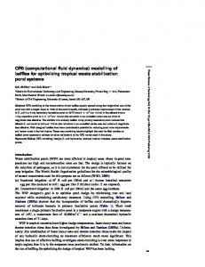
The predicted erosion depth results by using the stochastic rebound model are shown in Fig. 7. Good agreement between numerical simulation and measurement is found, especially in the area of highest 279


erosion at approx. 46° on the evaluation line. The reason for such behaviour can be seen in Figs. 8 ÷ 11. Comparing the streamwise velocity profiles before and after the elbow (Figs. 8 and 9), relatively large differences between stochastic and deterministic model can be seen. As the particle velocity is the main factor for erosion calculation (because of its exponent n, see Eq. (10), its proper prediction prior to the area of interest is of crucial importance. In most works dealing with solid particle erosion, particles are released at a very short distance before the erosion analysis spot and their velocity is assumed to be equal to the velocity of fluid, which is one of the main sources of errors when simulating erosion phenomena in real apparatus. In this particular geometry there is one elbow before our elbow of interest, so the numerical model must be capable of properly resolving particles velocities and concentration before the elbow where erosion is evaluated. For this reason the whole piping geometry upstream to the place of particle injection (Fig. 3) had to be taken for the simulation. 65 air particles, stochastic particles, deterministic

60 55

u (m/s)

50

s

45 40 35 30 25 -0.5

-0.4

-0.3

-0.2

-0.1

0 r/D

0.1

0.2

0.3

0.4


certainly after the first elbow, and the particle concentration in the vertical pipe is decisively altered for the deterministic model, Fig. 10. Due to its predetermined behaviour for every single particle without any stochastic influence from the wall roughness, the deterministic model tends to give unphysical results.

Figure 10 Relative particle concentration (kg/m³) at the Plane 1. a) stochastic rebound model, b) deterministic rebound model

The stochastic particle-wall rebound model, on the other hand, tends to equalize particle concentration along the pipe’s cross section. Due to stochastic virtual angle which is added to particle’s impact angle, particle’s velocity component normal to the wall can be even bigger after collision with the wall than before it. This pushes the particle concentration towards the centreline of pipes and channels, which is a more realistic behaviour, especially in horizontal pipes. This is also the reason why the erosion rate distribution along the elbow’s wall (Fig. 11) is not so sharp and predictable with the stochastic rebound model. The erosion depth on any other curve but the central evaluation line (Fig. 5) would probably not fit the experimental data with the deterministic model.

0.5

Figure 8 Air and particles streamwise velocity profiles taken at the plane 1 (before elbow)

0.5

air particles, stochastic particles, deterministic

0.4 0.3 0.2

r/D

0.1

Figure 11 Contours of the erosion rate E kg/(m2·s). a) stochastic rebound model, b) deterministic rebound model

0 -0.1 -0.2 -0.3 -0.4 -0.5 10

15

20

25

30 us (m/s)

35

40

45

50

Figure 9 Air and particles streamwise velocity profiles taken at the plane 2 (after elbow)

In Fig. 9 the difference between particle velocities calculated with stochastic and deterministic rebound model can be seen more clearly. Such a difference occurs 280

Besides particles velocity magnitude, the impact angle prior to erosion process is also of great importance, see Figs. 12 and 13. In the upper part of the elbow the carrier fluid is forced to change its direction, which leads to decreased fluids and particles velocity component normal to the wall (Fig. 12). Nevertheless, particles impact angle changes in this very area (middle of elbows outer wall section, Fig. 13), and particles hit the wall under the impact angle of approx. 23°. This is the limit value, see Eq. 11 and Tab. 1, and around this impact angle the maximum erosion occurs. Technical Gazette 21, 2(2014), 275-282


Figure 12 Mean particle velocity magnitude (m/s), stochastic rebound model


this reason it is important to take the history of particle movement into account long before the actual area of interest (erosion bend in this case). Very good agreement was found between numerical results and experimental data. Simulating solid particles erosion with the erosion model of Finnie [7] and the Virtual-wall model for particle-wall collisions shows good results in predicting potentially susceptible places in pneumatic conveying equipment, as well as in predicting the lifetime of such equipment. However, the erosion model still depends on numerous empirical coefficients, which have to be determined experimentally for different materials. Further work concerning the influence of secondary flow and the near-wall turbulence of the carrier fluid on solid particles as well as the change in wall roughness during the erosion process (time-dependent development of wall structure during erosion) is planned for the future. 7

Figure 13 Mean particle impact angle (°), stochastic rebound model

In Fig. 13 the effect of fluids secondary flow on the movement of particles can also be seen. At the place where the highest erosion at the centreline occurs, particles are deflected to the both sides of the centreline (two yellow-red spots in Fig. 13). As the relevant experimental data on the secondary flow influence on particle erosion cannot yet be found, the experimental validation of this phenomenon will be pursued later on. 6

Conclusions

In the present work, solid particles erosion in a pipe bend was investigated by means of numerical simulation and compared with experimental data from [1]. Special attention thereby was paid to the particles movement history in the pipe before the actual place of interest. Earlier works on experimental and numerical investigation of erosion showed that this is one of the main error sources when investigating erosion phenomena. Particle trajectories were calculated in Lagrangian reference frame by the Discrete Phase Model and the twoway coupled simulation method. Additional sub-model was implemented in the software in order to simulate particle-wall collisions more realistically. In wall-bounded flows, the realistic representation of particle-wall collisions is of crucial importance. The particles concentration profile in the cross-sectional area of the duct as well as the particle's velocity components are strongly influenced by the roughness of the wall. For Tehnički vjesnik 21, 2(2014), 275-282

References

[1] Chen, X. H.; McLaury, B. S.; Shirazi, S. A. Application and experimental validation of a computational fluid dynamics (CFD)-based erosion prediction model in elbows and plugged tees // Computers & Fluids. 33, (2004), pp. 1251– 1272. [2] Tsuji, Y.; Shen, N. Y.; Morikawa, Y. Lagrangian simulation of dilute gas-solid flows in a horizontal pipe // Advanced Powder Tech. 1, (1991), pp. 63–81. [3] Sommerfeld, M. Modelling of particle-wall collisions in confined gas-particle flows // Int. J. Multiphase Flow. 18, (1992), pp. 905–926. [4] Oesterlé, B. On heavy particle dispersion in turbulent shear flows: 3-D analysis of the effects of crossing trajectories // Boundary-Layer Meteorol. 130, (2009), 71. [5] Rubinow, S. I.; Keller, J. B. The transverse force on a spinning sphere moving in a viscous fluid // J. Fluid. Mech. 11, (1961), pp. 447–459. [6] Meng, H. C.; Ludema, K. C. Wear models and predictive equations – Their form and content // Wear. 181–183, (1995), pp. 443–457. [7] Finnie, I. Erosion of surfaces by solid particles // Wear. 3, (1960), pp. 87–103. [8] Tsuji, Y.; Morikawa, Y.; Tanaka, T.; Nakatsukasa, N.; Nakatani, M. Numerical simulation of gas-solid two-phase flow in a two-dimensional horizontal channel // Int. J. Multiphase Flow. 13, (1987), pp. 671-684. [9] Sommerfeld, M.; Huber, N. Experimental analysis and modelling of particle-wall collisions // Int. J. Multiphase Flow. 25, (1999), pp. 1457–1489. [10] Finnie, I.; Kabil, Y. H. On the formation of surface ripples during erosion // Wear. 8, (1965), pp. 60-69. [11] Wong, C. Y.; Solnordal, C.; Swallow, A.; Wang, S.; Graham, L.; Wu, J. Predicting the material loss around a hole due to sand erosion // Wear. 276-277, (2012), pp. 1-15. [12] Lester, D. R.; Graham, L. A.; Wu, J. High precision suspension erosion modeling // Wear. 269, (2010), pp. 449457. [13] Bilus, I.; Morgut, M.; Nobile, E. Simulation of Sheet and Cloud Cavitation with Homogenous Transport Models. // International Journal of Simulation Modelling. 12, 2(2013), pp. 94-106 [14] Hsu, F.H.; Wang, K.; Huang, C.T.; Chang, R.Y. Investigation on conformal cooling system design in injection molding. // Advances in Production Engineering & Management. 8, 2(2013), pp. 107-115

281



[15] Ternik, P.; Rudolf, R. Laminar Natural Convection of NonNewtonian Nanofluids in a Square Enclosure with Differentially Heated Side Walls. // International Journal of Simulation Modelling. 12, 1(2013), pp. 5-16 [16] Ansys Fluent 12.0 User Manual, ANSYS Inc., 2009. [17] Kahrimanovic, D.; Kloss, C.; Aichinger, G.; Pirker, S. Numerical study and experimental validation of particle strand formation // Progress in Computational Fluid Dynamics. 9, 6/7(2009), pp. 383-392. Authors’ addresses Halima Hadžiahmetović, M.Sc. Assistant, PhD candidate University of Sarajevo Faculty of Mechanical Engineering Sarajevo Department for Power Engineering and Processing Techniques Vilsonovo šetalište 9 71 000 Sarajevo Bosnia & Herzegovina E-mail: [email protected] Nedim Hodžić, Associate Professor University of Zenica Faculty of Mechanical Engineering Zenica Department for Power Engineering and Processing Techniques Fakultetska 1 72 000 Zenica Bosnia & Herzegovina E-mail: [email protected] Damir Kahrimanović, Researcher Johannes Kepler University, Institute of Fluid Mechanics and Heat Transfer Christian-Doppler Laboratory on Particulate Flow Modelling Altenbergerstrasse 69 4040 Linz Austria E-mail: [email protected] University of Sarajevo Faculty of Mechanical Engineering Sarajevo Department for Power Engineering and Processing Techniques Vilsonovo šetalište 9 71 000 Sarajevo Bosnia & Herzegovina E-mail: [email protected] Ejub Džaferović, Full Professor University of Sarajevo Faculty of Mechanical Engineering Sarajevo Department for Power Engineering and Processing Techniques Vilsonovo šetalište 9 71 000 Sarajevo Bosnia & Herzegovina E-mail: [email protected]

282

Technical Gazette 21, 2(2014), 275-282