Computational foundations of anthropomorphic ...

THÈSE En vue de l’obtention du

DOCTORAT DE L’UNIVERSITÉ FÉDÉRALE TOULOUSE MIDI-PYRÉNÉES Délivré par : l’Université Toulouse 3 Paul Sabatier (UT3 Paul Sabatier)

Présentée et soutenue le 1 septembre 2017 par :

Justin CARPENTIER

Computational foundations of anthropomorphic locomotion Fondements calculatoires de la locomotion anthropomorphe

Yacine CHITOUR Jean-Paul LAUMOND Nicolas MANSARD Stefan SCHAAL Alin ALBU-SCHÄFFER Christine CHEVALLEREAU Abderrahmane KHEDDAR Pierre-Brice WIEBER

JURY Professeur des Universités Directeur de Recherche Chargé de Recherche Professor Professor Directeur de Recherche Directeur de Recherche Chargé de Recherche

École doctorale et spécialité : EDSYS : Robotique 4200046 Unité de Recherche : Laboratoire d’Analyse et d’Architecture des Systèmes Directeur(s) de Thèse : Jean-Paul LAUMOND et Nicolas MANSARD Rapporteurs : Stefan SCHAAL et Alin ALBU-SCHÄFFER

Président du Jury Directeur de thèse Directeur de thèse Rapporteur Rapporteur Examinateur Examinateur Examinateur

..., je suis persuadé que la seule épreuve décisive pour la fécondité d’idées ou d’une vision nouvelles est celle du temps. La fécondité se reconnaît par la progéniture, et non par les honneurs. Alexandre Grothendieck, Les dérives de la "science officielle", 1988

Remerciements

Après trois merveilleuses années passées au LAAS-CNRS de Toulouse, il est temps pour moi de remercier les personnes qui ont largement contribué au succès de cette aventure – cela va sans dire qu’elles sont nombreuses et que je leur dois beaucoup. Je remercie chaleureusement mes deux directeurs de thèse : Jean-Paul Laumond et Nicolas Mansard. Merci de m’avoir ouvert les portes de cet univers incroyable qu’est la recherche; et en particulier la recherche en robotique. Cette collaboration a été très enrichissante et fort agréable. Je remercie également les protagonistes de l’ombre, et en premier lieu Philippe Souères, qui orchestre d’une main de maître l’équipe Gepetto. Mais aussi l’ensemble des Gepettistes, qui par leur bonne humeur et leur amitié ont fait de ces trois années une période très plaisante. Enfin, je ne saurais terminer cette salve de remerciements sans une pensée profonde à ma famille et à Thérèse. Merci à vous pour toutes ces années, passées et futures.

Contents Contents

i

List of Figures

v

Introduction

3

1 Anthropomorphic locomotion 1.1 Basic principles of anthropomorphic locomotion . . . . . . . . 1.1.1 The three spaces of movement . . . . . . . . . . . . . 1.1.2 Posture and placement . . . . . . . . . . . . . . . . . . 1.1.3 Actuation and under-actuation . . . . . . . . . . . . . 1.1.4 Physics of anthropomorphic locomotion . . . . . . . . 1.1.5 Equilibrium in locomotion . . . . . . . . . . . . . . . . 1.1.6 A first definition of anthropomorphic locomotion . . . 1.1.7 Walking as a particular mode of locomotion . . . . . . 1.2 Study of human locomotion . . . . . . . . . . . . . . . . . . . 1.2.1 A brief history of technical progresses in biomechanics 1.2.2 From measurements to estimation . . . . . . . . . . . 1.2.3 Orchestration of human locomotion . . . . . . . . . . 1.3 Anthropomorphic robots locomotion . . . . . . . . . . . . . . 1.3.1 Humanoid robots and passivity-based walkers . . . . . 1.3.2 Controlling locomotion of humanoid robots . . . . . . 1.4 Thesis overview . . . . . . . . . . . . . . . . . . . . . . . . . . 1.5 Associated publications and softwares . . . . . . . . . . . . .

. . . . . . . . . . . . . . . . .

. . . . . . . . . . . . . . . . .

. . . . . . . . . . . . . . . . .

. . . . . . . . . . . . . . . . .

5 5 5 6 8 8 9 10 10 11 12 13 14 15 16 16 17 18

2 Observability analysis and estimation of center of mass position 21 2.1 Motivation . . . . . . . . . . . . . . . . . . . . . . . . . . . . . . . . 21 2.2 Dynamic equations of under-actuated poly-articulated systems . . . 23 2.2.1 The under-actuated dynamics . . . . . . . . . . . . . . . . . . 24 2.2.2 The zero-moment point . . . . . . . . . . . . . . . . . . . . . 25 2.2.3 The central axis of the contact wrench . . . . . . . . . . . . . 25 2.2.4 The zero-moment point versus the projection on central axis of contact wrench . . . . . . . . . . . . . . . . . . . . . . . . . 26 2.3 Observability conditions of center of mass position . . . . . . . . . . 27 2.3.1 Observability with force/moment signals . . . . . . . . . . . . 28 2.3.2 Geometry-based CoM reconstruction . . . . . . . . . . . . . . 29 2.3.3 Validity of hypotheses, the spectral viewpoint . . . . . . . . . 31 2.4 The Linear Complementary Filter . . . . . . . . . . . . . . . . . . . 33 2.4.1 The input signals . . . . . . . . . . . . . . . . . . . . . . . . . 34 2.4.2 The design of complementary filters . . . . . . . . . . . . . . 34

ii

Contents 2.5

. . . . . . . . . . .

. . . . . . . . . . .

. . . . . . . . . . .

. . . . . . . . . . .

36 36 37 37 39 42 42 43 44 45 46

3 On the centre of mass motion in human walking 3.1 Motivation . . . . . . . . . . . . . . . . . . . . . . . . . . . . . 3.2 Material and methods . . . . . . . . . . . . . . . . . . . . . . . 3.2.1 Participants . . . . . . . . . . . . . . . . . . . . . . . . . 3.2.2 Data acquisition . . . . . . . . . . . . . . . . . . . . . . 3.2.3 Experimental protocol . . . . . . . . . . . . . . . . . . . 3.2.4 Center of mass reconstruction . . . . . . . . . . . . . . . 3.2.5 The curtate cycloid . . . . . . . . . . . . . . . . . . . . . 3.2.6 Segmentation of the gait . . . . . . . . . . . . . . . . . . 3.2.7 Fitting protocol . . . . . . . . . . . . . . . . . . . . . . . 3.3 Results . . . . . . . . . . . . . . . . . . . . . . . . . . . . . . . . 3.3.1 Fitting of the model . . . . . . . . . . . . . . . . . . . . 3.3.2 Link between model parameters and the subject’s height 3.3.3 The segmentation is embedded in the model . . . . . . . 3.4 Discussions . . . . . . . . . . . . . . . . . . . . . . . . . . . . . 3.4.1 Accuracy of the model . . . . . . . . . . . . . . . . . . . 3.4.2 An intuitive model with few parameters . . . . . . . . . 3.4.3 A stable descriptor and reliable predictor . . . . . . . . 3.4.4 A segmentation-free model . . . . . . . . . . . . . . . . 3.4.5 A useful model for walking gait analysis . . . . . . . . . 3.4.6 Limitations of the model . . . . . . . . . . . . . . . . . . 3.5 Conclusion and perspectives . . . . . . . . . . . . . . . . . . . .

. . . . . . . . . . . . . . . . . . . . .

. . . . . . . . . . . . . . . . . . . . .

. . . . . . . . . . . . . . . . . . . . .

49 49 51 51 51 52 52 52 53 53 56 56 57 58 58 58 59 59 60 60 61 61

4 Multi-contact locomotion of legged robots 4.1 Motivation . . . . . . . . . . . . . . . . . . . . . . . . 4.1.1 Reduced models . . . . . . . . . . . . . . . . . 4.1.2 Feasibility constraints . . . . . . . . . . . . . . 4.1.3 Outline of the chapter . . . . . . . . . . . . . . 4.1.4 Contribution . . . . . . . . . . . . . . . . . . . 4.2 Generic optimal control formulation . . . . . . . . . . 4.2.1 Contact model . . . . . . . . . . . . . . . . . . 4.2.2 Whole-body dynamics and centroidal dynamics

. . . . . . . .

. . . . . . . .

. . . . . . . .

63 63 64 65 66 66 66 67 67

2.6

2.7 2.8

Validation Study . . . . . . . . . . . . . . . . . . . . . 2.5.1 Generation of noisy data . . . . . . . . . . . . . 2.5.2 Spectral analysis of measurement errors . . . . 2.5.3 Description of the Kalman filter . . . . . . . . 2.5.4 Estimation and comparison with Kalman filter Applications . . . . . . . . . . . . . . . . . . . . . . . . 2.6.1 Walking . . . . . . . . . . . . . . . . . . . . . . 2.6.2 Running on a treadmill . . . . . . . . . . . . . 2.6.3 On the possible limitations . . . . . . . . . . . Related works . . . . . . . . . . . . . . . . . . . . . . . Conclusion and perspectives . . . . . . . . . . . . . . .

. . . . . . . . . . .

. . . . . . . .

. . . . . . . . . . .

. . . . . . . .

. . . . . . . . . . .

. . . . . . . .

. . . . . . . . . . .

. . . . . . . .

. . . . . . . .

Contents 4.2.3

4.3

4.4

4.5

4.6

4.7 4.8

Hierarchical decoupling between centroidal and manipulator dynamics . . . . . . . . . . . . . . . . . . . . . . . . . . . . . 4.2.4 State and control of the centroidal dynamics . . . . . . . . . 4.2.5 Generic optimal control formulation . . . . . . . . . . . . . . 4.2.6 From generic formulation to its implementation . . . . . . . . Learning feasibility constraints of the centroidal problem . . . . . . . 4.3.1 Handling feasibility constraints . . . . . . . . . . . . . . . . . 4.3.2 Learning the CoM reachability proxy . . . . . . . . . . . . . . 4.3.3 Empirical validation of the CoM proxy . . . . . . . . . . . . . Centroidal Wrench Cone Approximation . . . . . . . . . . . . . . . . 4.4.1 State of the art . . . . . . . . . . . . . . . . . . . . . . . . . . 4.4.2 Outer approximation . . . . . . . . . . . . . . . . . . . . . . . 4.4.3 Inner approximation . . . . . . . . . . . . . . . . . . . . . . . 4.4.4 Validation of the centroidal cone approximation . . . . . . . . Final formulation of the optimal control problem . . . . . . . . . . . 4.5.1 Tailored optimal control problem . . . . . . . . . . . . . . . . 4.5.2 Efficient resolution: the multiple shooting approach . . . . . Experimental results . . . . . . . . . . . . . . . . . . . . . . . . . . . 4.6.1 Description of the complete pipeline . . . . . . . . . . . . . . 4.6.2 Experiment 1 - long steps walking . . . . . . . . . . . . . . . 4.6.3 Experiment 2 - climbing up 10-cm high steps . . . . . . . . . 4.6.4 Experiment 3 - climbing up 15-cm high steps with handrail support . . . . . . . . . . . . . . . . . . . . . . . . . . . . . . Related works . . . . . . . . . . . . . . . . . . . . . . . . . . . . . . . Conclusion and perspectives . . . . . . . . . . . . . . . . . . . . . . .

iii

68 69 70 71 71 72 74 76 78 79 80 83 83 84 85 85 86 86 88 89 91 91 93

5 Conclusion and perspectives

95

Bibliography

99

List of Figures 1.1 1.2

1.3 1.4

1.5 1.6

The three media on earth. Each medium has its own physical properties which influence the evolution of the species living in it. . .

6

Unveiled human body. Illustration of the main skeletal muscles constitutive of the human body in the anatomical reference posture. Around 600 muscles put in motion the various articulations composing the human skeleton. . . . . . . . . . . . . . . . . . . . . .

7

Human postures. Four different postural configurations: arched back, lean forward, straight and lean backward. . . . . . . . . . . . .

8

Vestibular apparatus. Tomography 3D of the vestibular system. The yellow parts are the three semicircular canals in charge of sensing rotational movements. Otolithic organs are located at the base of the semicircular canal system. They sense the linear accelerations of the head. . . . . . . . . . . . . . . . . . . . . . . . . . . . . . . . . . . . .

10

Example of nominal walk. Two women walking normally on paving stones. . . . . . . . . . . . . . . . . . . . . . . . . . . . . . . .

11

Two examples of disequilibrium. The woman as well as the boy start to walk normally and then must watch their steps in order to avoid falling. . . . . . . . . . . . . . . . . . . . . . . . . . . . . . . .

11

1.7

Chronophotography of human motions. Superimposition of several photographies of a man walking and running, late 19th century. 12

1.8

An example of movement coordination. Chronophotography of Eadweard Muybridge throwing a disk, 1893. . . . . . . . . . . . .

1.9

14

Humanoid robots. Illustration of some remarkable humanoid robots. 15

1.10 Passivity-based walkers. Illustration of some popular passivity-based walkers. . . . . . . . . . . . . . . . . . . . . . . . . .

16

Scheme of the merging processus. The problem of merging measurements for CoM reconstruction in the presence of noises and modelling errors. . . . . . . . . . . . . . . . . . . . . . . . . . . . . .

22

Illustration of various notations. A graphic representation of the comparison between the central axis of the contact wrench and the ZMP. The ZMP part is depicted in red and shows the approximation made by the cart table model. The line joining the ZMP to the CoM of the cart-table model is parallel to the contact force vector. The central axis part is shown in blue. It is the line of minimal moment norm, also parallel to the contact force vector. . . . . . . . . . . . . .

27

2.1

2.2

vi

List of Figures 2.3

2.4 2.5 2.6

2.7

2.8

2.9

3.1

3.2

Illustration of the intuition on spectral distribution. A sketch representation of the spectral distribution of errors that would emerge from the naive reconstruction of CoM trajectory if we use only one signal (Geometry, Forces and projection of the CoM from Geometry onto the Contact Wrench Central Axis). The signal with the lowest error is then selected at each frequency bandwidth to constitute minimal-error fusion of these signals. . . . . . . . . . . . . Diagram of the CoM complementary filter for the three input signals. Bode diagrams of the three designed filters H1 , H2 and H3 , with f1 = 4 Hz and f2 = 0.4 Hz. . . . . . . . . . . . . . . . . . . . . . . . FFT of the error of each signal. In the top, the transform of the error between the real CoM position c and geometry-based estimation c˜. In the middle, the error between the second CoM time-derivative c¨ ˜¨. In the bottom, the and its estimation using force measurement c FFT of the error between the projection of the geometry-based CoM onto the central axis of the contact wrench Eq. (2.12) and the real CoM. For the three graphs, the x dimension is represented with solid red line, the y dimension with dotted green line and z dimension with dashed blue line. . . . . . . . . . . . . . . . . . . . . . . . . . . . . . On top, the reconstructed trajectory thanks to the complementary filter. On the middle, the two successive plots show the contribution of every signal to the reconstruction of CoM trajectory along the x and z axis respectively, together with the sum of the signals. On bottom, error between the ground truth measure of the CoM position and its reconstruction with the Kalman filter and the complementary filter. . . . . . . . . . . . . . . . . . . . . . . . . . . . . . . . . . . . . CoM position reconstruction for natural walking (red for x, green for y and blue for z). On the left, the reconstructed CoM in plain line and the CoM coming from geometry in dotted line. On the right, the force measurement during a short period. . . . . . . . . . . . . . CoM reconstruction for running on a treadmill (red for x, green for y and blue for z). On the left, the reconstructed CoM in plain line and the CoM coming from geometry in dotted line. On the right, one second of force measurement . . . . . . . . . . . . . . . . . . . . Illustration of the CoM trajectory in the sagittal plane during human walking. The CoM trajectory has a cycloidal pattern, described by a point on a wheel rolling at constant velocity on a flat surface. . . . . . . . . . . . . . . . . . . . . . . . . . . . . . Capture of the experiment room during the acquisition session. A male subject was instructed to walk barefoot in straight line at his comfort walking speed on two force platforms. Two force plates are firmly embedded in the floor and allows the reconstruction of the segmentation of the walking pattern. . . . . . . . . . . . . . . . . . .

32 34 35

38

40

42

43

50

51

List of Figures 3.3

3.4 3.5 3.6

3.7

3.8

3.9

vii

Illustration of the three types of cycloid. From top to bottom: normal cycloid, curtate cycloid and prolate cycloid. The last plot corresponds to the CoM trajectory in the sagittal plane. Its shape is very similar to the curtate cycloid. . . . . . . . . . . . . . . . . . . .

53

Illustrations of the segmentation of the gait (3.4(a)) and of the variability of the CoM during one single step (3.4(b)). . . . . . . . .

54

Illustration of the reconstruction of the center of mass trajectory (3.5(a)) and its reconstruction error (3.5(b)) during one stride. . . .

55

Mean and standard deviation of the reconstruction error for each subject. The mean reconstruction for all the subjects remains below 3.5mm with a maximal standard deviation of 1.5mm. . . . . . . . . .

56

On left, the scheme of the wheel with the notations of the model: R is the radius of the wheel while r is the distance of the point to the wheel center. On right, a scatter plot showing the evolution of the mean radius parameters R and r according to the subject’s sizes. The standard deviation of the parameters is low (below 5mm) for all the subjects. It appears that these two parameters are correlated to size of the subjects. . . . . . . . . . . . . . . . . . . . . . . . . . . . .

57

Evolution of the mean altitude z0 according to the subject’s size. The standard deviation of this parameter for each subject is very weak (below 2mm). Furthermore, the altitude is strongly correlated to the size of the subjects p ≤ 0.001 with a correlation coefficient of 0.87. .

58

Results of the fitting of θ with an affine approximation (3.9(a)) and evolution of the mean angular velocity regarding to the subject height (3.9(b)). . . . . . . . . . . . . . . . . . . . . . . . . . . . . . . . . . .

59

3.10 Bar graph of the prediction error of the time instants of start and end of the double support phases. In average, the two instants defining the double support are well captured by the model with only few milliseconds of errors. . . . . . . . . . . . . . . . . . . . . . . . . . .

60

3.11 The Yoyo-Man model opens promising research routes to continue exploring the computational foundations of human and humanoid walking. Most existing walking controllers for humanoid robots consider a bottom-up approach based on the control of the so-called Zero Moment Point (ZMP) [Vukobratović and Borovac, 2004, Kajita et al., 2003]. With the Yoyo-Man model, we suggest new plausible walking bottom-up control schemes that benefit from the knowledge of the Centre of Mass motion. . . . . . . . . . . . . . . . . . . . . . .

61

4.1

Illustration of HRP-2 robot and TALOS robot making contacts with their environment. The green “ice-cream” cones are dispatched on the 4 vertices of the feet, symbolizing the friction cones with friction coefficient of value 0.3. . . . . . . . . . . . . . . . . . . . . . . . . . .

64

viii

List of Figures

4.2

Illustration of the probability density distribution of the CoM w.r.t. the right foot frame of HRP-2, projected along the three axis X,Y,Z. The first row corresponds to the ground truth distribution estimated through KDE (20000 points). Next rows depict the learned GMM with respectively 5, 7 and 13 kernels in the mixture. . . . . . . . . . 4.3 Evolution of the KL divergence between the KDE distribution and GMMs of different sizes for the four end-effectors of the HRP-2 robot. 4.4 Illustration of the probability density distribution of the CoM w.r.t. the right foot frame of TALOS, projected along the three axis X,Y,Z. The first row corresponds to the ground truth distribution estimated through KDE (20000 points). The second row depicts the learned GMM with 4 Gaussian kernels in the mixture. The axes have the same scale than in Fig 4.2. . . . . . . . . . . . . . . . . . . . . . . . 4.5 Checking of the CoM independence hypothesis for various scenarios. (Left) contact configurations and (right) corresponding level sets of the CoM occupancy measures, with ground truth in solid lines and approximations in dashed lines. On the first row, the robot makes two contacts with the stairs while on the second one, the robot is also handling the handrail. On the last row, the robot is making 4 contacts. . . . . . . . . . . . . . . . . . . . . . . . . . . . . . . . . . . 4.6 Illustration of the procedure to build the outer approximation of the CWC from the collection of rays coming from the linearization of the contact cones. . . . . . . . . . . . . . . . . . . . . . . . . . . . . . . . 4.7 Illustration of the contact wrench approximations for scenarios of Fig. 4.5. The exact CWC and its linear approximation closely matches. The outer approximation is obtained with α = 1, and the inner approximation with α = 0.2. The approximation α = 0.3 is an efficient trade off. . . . . . . . . . . . . . . . . . . . . . . . . . 4.8 Comparison of the state trajectories obtained with either the force-based OCP (simple and exact 3D cones, nonminimal parameters – af ) or the motion-based OCP (approximate 6D cone, minimal 6D parameters – ac ). In theory, the optimum of both problems should be the same, however the numerical properties of each OCP leads to minor variations. The CoM trajectories have similar shape but the dynamic marginally varies. The motion-based OCP leads to marginally smoother trajectories. Much more oscillations appear at the angular momentum level when optimizing the forces, but they mostly correspond to numerical noise. . . . . . 4.9 Projection of the CoM trajectory inside the right foot frame with and without taking into account the log-pdf term in the cost function. The level set corresponds to the GMM distribution used in our OCP. 4.10 Snapshots of the climbing up 10-cm high steps motion with the HRP-2 robot. . . . . . . . . . . . . . . . . . . . . . . . . . . . . . . .

77 77

78

79

80

84

87

89 90

List of Figures 4.11 Snapshots of the climbing up 15-cm high steps motion with the HRP-2 using the handrail. . . . . . . . . . . . . . . . . . . . . . . . . 4.12 Snapshots of the climbing 15-cm high steps motion with handrail by the TALOS robot in simulation. . . . . . . . . . . . . . . . . . . . . .

ix

90 90

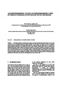
L’homme qui marche (The Walking Man) An interpretation of how human beings walks by Gustave Rodin, 1907.

L’homme qui marche I (The Walking Man I) An other interpretation of how human beings walks by Alberto Giacometti, 1961.

Introduction

H

uman body is an extraordinary machine. He is extraordinary because he is provided with a consciousness. This consciousness allows him to realize that he is a machine able to move in the world thanks to its own gesticulation. Yet this consciousness does not allow him to get a direct insight into the underlaying mechanisms. Indeed, human consciousness is raised through the flow of actions. And those actions do not occur inside the motor space, at the muscles level, but rather in the physical space, the space where human movements happen. For instance, choreographers do not talk to muscles of dancers. But they talk to dancers about the movements to perform inside the physical space. And dancers play these movements with their own feeling, without controlling individually each muscle. The same applies for locomotion. Usually, humans walk just as they breathe, in an unconscious fashion. Which machinery is at the origin of this unconscious orchestration in human locomotion? This question remains an enigma. Some answers and interpretations have already been suggested by various scientific communities like biomechanics, physiology, neurosciences, medicine, etc. This thesis contributes to this endeavor by proposing a study framework and by highlighting a particular coordination which occurs during walking. Unlike choreographers, roboticists directly talk to the actuators of robots. They can individually control each of their actuators. Hence, they have a direct influence on the motions of limbs, which leads to the whole displacement of robots. Yet, these actuators must not be controlled separately but jointly, in order to produce the right orchestration allowing these displacements. Several frameworks have been proposed to achieve this coordination. But they remain limited to particular environments. A common wish is expressed inside the robotics community to enable legged robots to move in autonomous manner inside rough and heterogeneous locations. This thesis provides an initial response to this wish by introducing an original and versatile framework for multi-contact locomotion of legged robots.

Chapter 1

Anthropomorphic locomotion Contents 1.1 1.2 1.3 1.4 1.5

Basic principles of anthropomorphic locomotion Study of human locomotion Anthropomorphic robots locomotion Thesis overview Associated publications and softwares

5 11 15 17 18

oving by its own is the essence of living beings. Locomotion is the faculty for animals or mechanical systems to move from one place to another. It is the main characteristic which differentiates the animal reign from the vegetal one. Animals have the ability to move freely while plants are condemned to fixity by their roots. On earth, three different media are the substrates for locomotion: aquatic, terrestrial and aerial environments illustrated in Fig. 1.1. For each medium, nature through evolution has given birth to various morphologies adapted to the physical properties of the medium. In air for instance, evolution has resulted in wings to allow birds to support their weight and then flight. On land, legged morphologies exhibit a remarkable ease to cross gaps, run on uneven surfaces or just walk on a wide variety of textured terrains (sandy beach, grassland, steep ground, etc). This great ease to move might explain in some sense why robotics engineers have been aspiring to build legged machines for decades to overcome the intrinsic limitations of wheeled machines.

M

1.1

Basic principles of anthropomorphic locomotion

In this thesis, we focus on a particular type of legged locomotion called anthropomorphic locomotion. It corresponds to the locomotion of systems having a human-like morphology. Thereon, human and humanoid locomotions are the two main instances of anthropomorphic locomotion. In what follows, we introduce the main vocabulary and principles commonly employed in the context of anthropomorphic locomotion. All the concepts detailed below are familiar to everyone because they translate in words the way he or she - as human beings behaves everyday.

1.1.1

The three spaces of movement

Human beings and humanoid robots share the same ambient space, where physical laws govern the motion of bodies. We refer the ambient space as the physical space. It is the space where all the actions occur. For instance, when a human holds a hammer to nail, the action of nailing takes place in the physical space.

6

Chapter 1. Anthropomorphic locomotion

(a) Bee in flight

(b) Cheetah running

(c) Sea turtle swimming

Figure 1.1: The three media on earth. Each medium has its own physical properties which influence the evolution of the species living in it. In order to hold the hammer or to nail, the articulations of the arm and the shoulder are either stiffened or put in movement thanks to skeletal muscles. Skeletal muscles are soft tissues, linking two consecutive bones together and producing force and motion as a result of their contraction. Fig. 1.2 shows the muscle structure of humans in the anatomic position. In the context of humanoid robots, biological muscles are replaced by actuators (electrical motors, hydraulic pistons, etc). Both muscles and actuators belong to the so-called motor space. It is the space of control, where the central nervous system or computers make specific orders for the purpose of animating the poly-articulated structure. Finally, in order to precisely put the head of the hammer onto the nail, humans must be aware of the precise location of the nail with respect to themselves. This precise location is provided by exteroceptive sensory receptors which convey stimuli towards the central nervous systems. All these receptors provide information about the outside world and form what are called exteroception or exteroceptive senses: vision, audition, taste, olfaction and touch, including equilibrioception through the vestibular system. In addition to the exteroception, the human body is provided by proprioceptors which supplies internal state information: stretch in the muscles, lengthening of ligaments, etc. Proprioceptors constitute the proprioception. All those aforementioned stimuli project into the so-called sensorial space. For their part, humanoid robots are not yet equipped with biological but electromechanic sensors: force sensors, tactile cells, cameras, accelerometers for the exteroception and encoders, load cells for the proprioception, just to name a few.

1.1.2

Posture and placement

As anthropomorphic systems, humans and humanoid robots share a common morphology: both of them are roughly equipped with two arms, two legs, one torso and one head. Although similar in terms of morphology, human body owns much more degrees of freedom than current humanoid robots. One counts around 360 articulations in the human body against more or less 30 joints for most humanoids. All those degrees of freedom define the posture, namely the shape of the body. Yet, the postural information is not sufficient to describe the location of the body in the physical space. The missing information corresponds to the notion

1.1. Basic principles of anthropomorphic locomotion

7

Figure 1.2: Unveiled human body. Illustration of the main skeletal muscles constitutive of the human body in the anatomical reference posture. Around 600 muscles put in motion the various articulations composing the human skeleton.

8


Figure 1.3: Human postures. Four different postural configurations: arched back, lean forward, straight and lean backward. of placement. A placement characterizes the position and the orientation of a particular corporal segment, like the head, the chest or the waist for instance. The combination of posture and placement variables is then sufficient to solely describe the individual segment locations inside the physical space.

1.1.3

Actuation and under-actuation

As mentioned earlier, the human posture is put in movement by muscles. In total, there are over 600 muscles to animate the posture. In some sense the human body can be considered as an over-actuated system: there are more actuators than degrees of freedom to control. In contrast, there is no actuator or organ to directly operate the placement quantity. The same applies for biking for instance. The rider can move forward thanks to the pedal and turn with the handlebar. But it is impossible for he or she to directly achieve a lateral movement. The biker has to make some maneuvers by combining the effect of the pedal with the change in the direction. For this reason, anthropomorphic bodies and bicycles are also known as under-actuated systems.

1.1.4

Physics of anthropomorphic locomotion

Anthropomorphic locomotion is first and foremost a dialogue with gravity. Human skeleton continuously experiences gravity, with an influence of variable strength

1.1. Basic principles of anthropomorphic locomotion

9

which depends on the context. For instance, body suffers more from the effect of gravity when it travels a rolling countryside rather than when it walks on a flat ground. Gravity acts on every single segment composing the body. Its effect depends directly on the shape and the mass distribution of segments. The necessity of contact interaction A remaining question is how do humans control their placement? How do they transform their inter-limb motions into displacement? The answer lies in the physical interaction between the human body’s extremities and the environment. For instance, when feet touch the ground, they produce a deformation of the ground structure at the atomic scale. This atomic structure withstands the pressure developed by the feet. As a consequence, feet stick to the atomic structure and it produces in return an equal and opposite reaction which operates on the body placement. This physical interaction acts directly on the linear and angular momenta, allowing a displacement of the center of mass. The notion of centroidal dynamics The shape and the mass distribution of segments together with the posture define entirely the center of mass of the body. It is also known as the center of gravity, namely a virtual point where the action of gravity is condensed. It is a geometric quantity. Motions of body segments through the variations of posture affect the linear and angular momenta of the limbs. They relate the quantity of motion in translation and rotation of the segments, i.e. in some ways the kinetic energy involved in the motion. However the anthropomorphic body can be reduced to a single point-mass model defined by the combination of all segments linear and angular momenta. The position of the reduced system then coincides with the body center of mass position. This reduction is called centroidal dynamics model. The dynamics of this point-mass system is only governed by the contact interaction with the ground. In other words, the forces exerted by the muscles indirectly affect the centroidal dynamics through contacts. In this thesis, we highlight the leading role played by the centroidal dynamics in human locomotion, but also for the generation of locomotor trajectories for humanoid robots.

1.1.5

Equilibrium in locomotion

Equilibrium is the fact to maintain balance, or in other terms, the fact to avoid any unexpected fall. Many scenarios can lead to fall: a bad coordination of segmental motions, an unexpected contact, etc. Equilibrium is a pre-requisite to accomplish other skills, like reaching movements or locomotion. For all these reasons, equilibrium plays a central role in the understanding and the generation of anthropomorphic locomotion.

10


Figure 1.4: Vestibular apparatus. Tomography 3D of the vestibular system. The yellow parts are the three semicircular canals in charge of sensing rotational movements. Otolithic organs are located at the base of the semicircular canal system. They sense the linear accelerations of the head. Senses of equilibrium Multiple sensorial inputs contribute to the sense of equilibrium: visual inputs, vestibular inputs as well as some postural information provided by mechanoreceptors. Among all those receptors, the vestibular system has an important function. Indeed, it is the only sense which has no dedicated area in the brain, unlike vision or audition. But the vestibular afferents are directly processed by other cortical area devoted to other senses like vision or proprioception. This leads for example to the vestibulo-ocular reflex, where eyes move according to the afferent signals from vestibular apparatus. It allows to stabilize images on the retina and it simplifies the data process for visual interpretation. Vestibular apparatus The vestibular system, depicted in Fig. 1.4, is a component of the the inner ear which is located just after the auditory canal. It is composed of two main parts. The first one is composed of three semicircular canals (yellow part in Fig. 1.4). They detect rotational movements of the head. At the base of the semicircular canal system are the otolithic organs. They sense the linear accelerations of the head.

1.1.6

A first definition of anthropomorphic locomotion

From the previous statements and observations, we can establish a first definition of anthropomorphic locomotion. Anthropomorphic locomotion is the faculty for a system to modify its placement, i.e. to perform a displacement, by the motion of body segments together with the contact interaction of the limb extremities with the environment. To produce the right contact reactions that keeps from falling, the body segments must be actuated with a particular orchestration, driven by the nervous system under the influence of sensorial stimuli.

1.1.7

Walking as a particular mode of locomotion

Among all modes of locomotion (running, climbing, crawling, etc.), walking is the most familiar to us. It is one of the first modes that we experimented during infancy

1.2. Study of human locomotion

11

Figure 1.5: Example of nominal walk. Two women walking normally on paving stones.

Figure 1.6: Two examples of disequilibrium. The woman as well as the boy start to walk normally and then must watch their steps in order to avoid falling. after crawling. It also the mode we use most of the time. However, we do not walk all the time with the same gait, with the same pattern. We may distinguish between two types of walking. The walk where humans have to look at their steps when the ground is too uneven. And the thoughtless walking, that is when humans walk without thinking about it, i.e. without looking where they have to place their feet. It is a reflexed-base walk. This two types of walking are illustrated in Fig. 1.5 and Fig. 1.6. For both types, walking is defined by the succession of single and double support phases. During the single support phase, the stance leg carry all the body weight while the other leg swings forward from the hip. Then the swing foot hits the ground with the heel, that marks the beginning of the double support phase. During a cycle, the stance foot describes a rolling motion from the heel through the toe.

1.2

Study of human locomotion

The orchestration at the origin of human locomotion remains largely a mystery. Exploring this orchestration is a multidisciplinary topic of research involving for decades many scientific disciplines as neurosciences, physiology, biomechanics, medicine and of course robotics. Despite the complexity of the locomotion

12


Figure 1.7: Chronophotography of human motions. Superimposition of several photographies of a man walking and running, late 19th century. process, technical progresses have allowed some important breakthroughs in its understanding. Among these breakthroughs, there are electromyography to measure electrical muscle activities, electroneurography and microneurography to record nerve impulses but also techniques as motion capture systems, to analyze the global motion of human body. In the following, we only consider human locomotion through the prism of biomechanics. Biomechanics studies mechanical properties of biological systems. It is an old scientific discipline with a long history.

1.2.1

A brief history of technical progresses in biomechanics

The first scientific studies on human mechanics date back to Renaissance period. It was at this time that mechanics appeared as a scientific discipline at the instigation of Galilee. The first book describing the mechanical organization of the human body, in other words human biomechanics, was written by Giovanni Alfonso Borelli in 1680 and entitled De motu animalium (Movement of Animals). In his book, Borelli compared the human body to a machine composed of levers and strings, representing bones and muscles respectively, similar to a marionette. It was not until the beginning of 19th century that the first experimental studies on human locomotion appeared thanks to Wilhelm and Eduard Weber [Weber and Weber, 1836]. They measured some of the main features of human walking: step length and pattern frequency as well as a rough estimate of the center of mass position in standing position. Yet, the study of human locomotion increased thanks to technical evolutions. The first technological step forward was achieved by Eadweard Muybridge with the invention of chronophotography in 1878. This technique consists in a

1.2. Study of human locomotion

13

superimposition of several photographies in order to temporally decompose motions. Fig. 1.7 depicts two examples of chronophotography. In some sense, it was the first motion capture system. The first electromyography was achieved in the twenties by Wachholder [Sternad, 2002]. He was investigating the coordination of muscular activities during walking. In his studies, he precisely found out which muscles are involved in the processus of walking. Last, the first force plate was introduced by Elftman Herbert in 1938 [Elftman, 1938]. It consisted in a platform suspended by four springs. The compression of the springs allow to estimate the forces acting on the platform. All modern plates follow the same design principles. All these historical notes allow us to better understand how human locomotion experiments were influenced by technical advancements. A wider overview on the history of human locomotion studies is addressed in Latash and Zatsiorsky [2001]. Today, most of modern biomechanics laboratories are equipped with a motion capture system, one or several force plates, electromyographic sensors, wearable inertial measurement units, etc. Nevertheless, measurements coming from these sensors are not usable in their raw states and must be processed first.

1.2.2

From measurements to estimation

Biomechanics sensors provide raw measurements: force and torque signals from the force plates, 3d positions of reflective markers from the motion captures, muscular activities from electromyography sensors, etc. All those measurements also convey noise of various levels depending on the technology employed and the positioning of sensors. For instance, 3d positions of reflective markers are related both to the movement of the supporting segment, but also to the intermediate skin movement, leading to unwanted artifacts. In addition, measures of marker positions through visual devices adjoin extra uncertainties. Ideally, one’s would like to only keep the interesting part of signals and remove the components due to artifacts. Yet it is hard to guess what is the contribution of noises in raw measurements. To overcome this issue, researchers in biomechanics tend to reduce input noise levels by using standard methods from signal processing, like low or high pass filtering, etc. However, there is no guaranty that noise is located in a precise spectral bandwidth or that useful information will not be affected by filtering. Another important issue concerns the observability properties of the physical quantities from measurements. In other terms, is it possible to entirely reconstruct all informations from the given measurements? If we refer to the classic textbook of biomechanics methodologies [Winter, 2009, Robertson et al., 2013], this issue is under-estimated inside this community. On the contrary, it is a crucial topic for roboticists to allow the feedback control of complex robots from sensor measurements. If a physical quantity is not observable, that means it is impossible to retrieve its values from any measurement. Then, any conclusion dealing with non-observable quantities is dubious.

14


Figure 1.8: An example of movement coordination. Chronophotography of Eadweard Muybridge throwing a disk, 1893. Nevertheless, observability conditions are not sufficient. The practical introduction of estimators is essential to ensure the complete reconstruction of observable quantities. There exists a wide range of estimators. They usually merge various signals in order to reconstruct desired quantities. They allow the estimation of bias, the reject of noises, etc. Biomechanics methodologies do not yet include such tool to increase likelihood of data extracted from measurements. One of the contribution of this thesis is to establish the observability conditions of the center of mass position, i.e. we exactly define what are the components of the center of mass position which can be estimated using standard protocols of biomechanics. In addition to that, we introduce a new estimator based on complementary filtering to reconstruct this position of the center of mass. The originality of this estimator is to merge common measurements (force plate signals, motion capture data) according to their frequency resolutions. This estimator is also granted to provide the entirety of the signal by construction.

1.2.3

Orchestration of human locomotion

As mentioned earlier, human locomotion is a complex process involving hundreds degrees of freedom as well as hundreds muscles. Encompassing all the small details of this process certainly goes beyond scientific understanding. In spite of this complexity, it is still possible to observe either muscles coordinations or limb coordinations when achieving some tasks [Flash and Hogan, 1985]. For instance, Fig. 1.8 illustrates the throw of disk by Eadweard Muybridge. On this chronophotography, we observe that his right hand is forward while his right leg and left hand are positioned backward. This corresponds to a coordination of the upper and lower limbs to ensure the balance of the body. In the context of locomotion, several orchestration principles have already been observed. It has been shown in Barliya et al. [2009] that the elevation angles of the lower limb segments lie in a plane during walking. In Pozzo et al. [1990], the authors

1.3. Anthropomorphic robots locomotion

(a) Atlas Boston Dynamics

(b) HRP-2 Kawada Industries

15

(c) TORO Deutsches Zentrum für Luftund Raumfahrt

Figure 1.9: Humanoid robots. Illustration of some remarkable humanoid robots. highlight the stabilization of the head orientation during locomotion. In Herr and Popovic [2008], the cancellation of the angular momentum quantity during walking is brought out. In this thesis, we highlight another orchestration principle based on the position of the center of mass. Studies on the center of mass trajectory during walking are numerous inside the biomechanics community [Farley and Ferris, 1998, Orendurff et al., 2004, Lee and Farley, 1998]. But none of them has clarified the geometric nature of this trajectory. We experimentally show that the center of mass trajectory follows a cycloidal trajectory in the sagittal plane during nominal walk. We also expose that the parameters of the cycloidal pattern are only affected by the size of the body. All these results are based upon acquisition of walking motions on several subjects.

1.3

Anthropomorphic robots locomotion

The shape of anthropomorphic robots are largely inspired from human beings. But it is essentially the only feature that they have in common. Indeed, their actuation systems completely differ from the musculoskeletal architectures of humans. They are also equipped with few sensors in comparison with human beings. There is still no biologically-inspired humanoids even if some progresses are made to create artificial muscles [Simaite et al., 2016]. Current humanoids are simply machines equipped with two arms and two legs, provided with actuators, electromechanical sensors and computers. Each movement of these machines is generated by dedicated algorithms. For instance, the algorithm devoted to the drilling task is different from the algorithm in charge of locomotion tasks. Even for locomotion tasks, walking or climbing stairs are not generated by the same algorithm. In fact, there is still no unique formulation to tackle the locomotion problem globally.

16


(a) Mike Delft University

Figure 1.10: Passivity-based passivity-based walkers.

1.3.1

(b) Cornell ranger Cornell University

walkers.

Illustration of some popular

Humanoid robots and passivity-based walkers

Among anthropomorphic robots, the robotics community tends to make a strict distinction between humanoid robots Fig. 1.9 and passivity-based walkers Fig. 1.10 . On one side, passive walkers are rather simple machines, whose aim is to reach similar performances than humans for walking in terms of energy consumption. They are only equipped with few and quite limited actuators. On the other side, humanoid robots are versatile and fully actuated machines whose goals are not only to move but also to operate on various contexts. Fig. 1.9 and Fig. 1.10 show a sample of humanoid robots and passivity-based walkers, that are among the most dominant experimental platforms developed for research purposes. Robotics engineers tend to create distinct algorithms to operate on those two classes of robots, and especially in the context of locomotion. But these two classes of robots are governed by the similar dynamical equations of motion. Then it seems possible to set up a unified formulation at least for locomotion. In recent works, we have introduced a unified framework for simultaneous design and control of anthropomorphic robots [Saurel et al., 2016, Buondonno et al., 2017]. It allows to compute the best robot architecture (mass distribution, segment lengths, etc) as well as the parameters of the actuators and their commands in order to achieve cyclic motions while minimizing energy consumption. It is a first step towards the co-design of humanoid robots and passivity-based walkers.

1.3.2

Controlling locomotion of humanoid robots

Ensuring locomotion of humanoid robots is a quite challenging aim that has been motivating roboticists for decades. One of the major challenges is the balance control of humanoid robots while they move. To ensure this balance, the limbs of humanoids must be coordinated to produce adequate contact forces in order to

1.4. Thesis overview

17

avoid slippage or any unexpected contact breaking. To meet this purpose, two broad views have emerged. The first view considers the complete dynamics of the system as a whole. This means that each degree of freedom is individually controlled to participate to the whole-body orchestration. Several mathematical frameworks can be used to meet this behavior: numerical optimal control [Tassa et al., 2012, Mombaur, 2001, Lengagne et al., 2013], hybrid zero dynamics [Westervelt et al., 2007], just to name a few. Yet, whole-body formulations lead to high-dimensional problems and then require intensive computations, out of scope of modern computers. The second view is based on a decoupling strategy which consists in first dealing with a low dimensional problem based on a reduced template models (e.g. the linear inverted pendulum) and then compute a whole-body control that follows this reduced dynamics. The most popular example of such strategy is the cart-table model introduced by Kajita et al. [2003]. Nevertheless, most of existing template models are based on some restrictive hypotheses that limit their range of applications. In In addition, reduced models are generally not able to cope with the constraints of the robot complete model as torque bounds or kinematics limits for instance. In this thesis, we introduce an original formulation able to quickly compute multi-contact locomotion trajectories for any legged robot on arbitrary terrains. This formulation relies on a generic template model based on the centroidal dynamics. This dynamics is exact and our formulation is thus not limited by arbitrary assumption. It then leads to generic locomotion on any environment: flat floor, rough terrain, stair with and without handrails, and by extension, standing up, sitting down, running, jumping, etc. We also introduce a generic procedure to handle feasibility constraints due to the robot whole body as occupation measures, and a systematic way to approximate them using off-line learning in simulation. We illustrate the effectiveness and the versatility of the approach on two humanoid robots with several multi-contact scenarios both in reality and in simulation.

1.4

Thesis overview

Rational In this thesis, we argue that the centroidal dynamics, as a reduction of the full physical system, is a keystone of anthropomorphic locomotion. It is a necessary key to study the orchestration of human locomotion in the context of biomechanics studies. This centroidal dynamics is also the necessary and sufficient dynamics to synthesize the locomotion of humanoid robots in heterogeneous environments.

Thesis organization This thesis is composed of three main contributions. Two of three contributions are already published in international journals and one is partially published in

18


conferences and it is still under the review process. To keep the developments clear and let each contribution independent from the rest of the manuscript, we decided to present the related publications in their original versions.

Chapter organization This manuscript is organized as follows. In a first time, we establish in Chapter 2 the observability conditions of the center of mass position. These observably conditions allow us to introduce an estimator of the center of mass position dedicated to anthropomorphic locomotion. Based on this estimator, we experimentally show in Chapter 3 that the center of mass follows a cycloidal pattern in the sagittal plane during nominal walk. We also demonstrate that the cycloidal parameters is only affected by the size of the subjects. In Chapter 4, we present our original formulation for the multi-contact locomotion of legged robots based on the centroidal dynamics associated to occupation measures to reflect whole-body constraints. Finally, the conclusive Chapter 5 draws global perspectives and gives a personal view on future impacting research directions.

1.5

Associated publications and softwares

This thesis has led to several publications, all of them dealing with the locomotion of anthropomorphic systems.

Journal articles ♣ Justin Carpentier, Mehdi Benallegue, Nicolas Mansard, and Jean-Paul

Laumond. Center of Mass Estimation for Polyarticulated System in Contact — A Spectral Approach. IEEE Transactions on Robotics (TRO), 2016a; ♣ Jean-Paul Laumond, Mehdi Benallegue, Justin Carpentier, and Alain

Berthoz. The Yoyo-Man. International Journal of Robotics Research (IJRR), 2017; ♣ Justin Carpentier, Mehdi Benallegue, and Jean-Paul Laumond. On the

centre of mass motion in human walking. International Journal of Automation and Computing, 2017a.

Conference articles ♣ Olivier Stasse, Thomas Flayols, Rohan Budhiraja, Kevin Giraud-Esclasse,

Justin Carpentier, Andrea Del Prete, Philippe Souères, Nicolas Mansard, Florent Lamiraux, Jean-Paul Laumond, et al. Talos: A new humanoid research

1.5. Associated publications and softwares

19

platform targeted for industrial applications. In IEEE-RAS International Conference on Humanoid Robots (Humanoids), 2017; ♣ Gabriele Buondonno, Justin Carpentier, Guilhem Saurel, Nicolas Mansard,

Alessandro De Luca, and Jean-Paul Laumond. Optimal design of compliant walkers. In IEEE/RSJ International Conference on Intelligent Robots and Systems (IROS), 2017. ♣ Justin Carpentier, Rohan Budhiraja, and Nicolas Mansard.

Learning feasibility constraints for multi-contact locomotion of legged robots. In Robotics: Science and System (RSS), 2017b;

♣ Justin Carpentier, Steve Tonneau, Maximilien Naveau, Olivier Stasse, and

Nicolas Mansard. A versatile and efficient pattern generator for generalized legged locomotion. In IEEE International Conference on Robotics and Automation (ICRA), 2016b; ♣ Maximilien Naveau, Justin Carpentier, Sébastien Barthelemy, Olivier

Stasse, and Philippe Souères. METAPOD—Template META-programming applied to dynamics: CoP-CoM trajectories filtering. In IEEE-RAS International Conference on Humanoid Robots (Humanoids), 2014; ♣ Jean-Paul Laumond, Mehdi Benallegue, Justin Carpentier, and Alain

Berthoz. The yoyo-man. Research (ISRR), 2015;

In 17th International Symposium on Robotics

♣ Guilhem Saurel, Justin Carpentier, Nicolas Mansard, and Jean-Paul

Laumond. A simulation framework for simultaneous design and control of passivity based walkers. In 2016 IEEE International Conference on Simulation, Modeling, and Programming for Autonomous Robots (SIMPAR), 2016; ♣ Justin Carpentier, Mehdi Benallegue, Nicolas Mansard, and Jean-Paul

Laumond. A kinematics-dynamics based estimator of the center of mass position for anthropomorphic system – a complementary filtering approach. In IEEE-RAS International Conference on Humanoid Robots (Humanoids), 2015a; ♣ Justin Carpentier, Andrea Del Prete, Nicolas Mansard, and Jean-Paul

Laumond. An analytical model of rolling contact and its application to the modeling of bipedal locomotion. In IMA Conference on Mathematics of Robotics, 2015b.

Submitted article ♣ Justin Carpentier and Nicolas Mansard.

Multi-contact locomotion of legged robots. Technical report, LAAS-CNRS, 2017. Submitted to IEEE Transactions on Robotics (TRO) (May 2017);

20


Softwares This thesis has also led to the development of Pinocchio1 [Carpentier et al., 2015–2017], a C++ library for efficient computations of forward and inverse dynamics of poly-articulated systems. This library is a trade off between HuManS [Wieber et al., 2006] for efficient computations and RBDL [Felis, 2017] for its simplicity and versatility to use. This novel library is now at the hearth of many software frameworks developed by the Gepetto team like the Stack of Tasks [Mansard et al., 2009] and the Humanoid Path Planner [Mirabel et al., 2016].

1

https://github.com/stack-of-tasks/pinocchio

Chapter 2

Observability analysis and estimation of center of mass position

Contents 2.1 2.2 2.3 2.4 2.5 2.6 2.7 2.8

Motivation Dynamic equations of under-actuated poly-articulated systems Observability conditions of center of mass position The Linear Complementary Filter Validation Study Applications Related works Conclusion and perspectives

21 23 27 33 36 42 45 46

his chapter discusses the problem of estimating the position of the center of mass for poly-articulated systems (e.g. humanoid robots or human body), which make contact with their environment. The measurements we consider are the interaction forces (typically coming from ankle force sensors or force plates) and the kinematic reconstruction (e.g. mass positions) estimated from a dynamical model of the system together with the information provided by encoders or motion capture systems. We first study the observability of the center-of-mass position using these measurements. We show that the accuracy domain of each measurement can be easily described through a spectral analysis. We then introduce an original approach based on complementary filter theory to efficiently merge these input measurements and obtain an accurate estimation of the center-of-mass position. This approach is extensively validated in simulations by using a model of a humanoid robot. These simulations confirm the spectral analysis of the signal errors. In particular, we show that the complementary filter offers a lower average reconstruction error than the classical Kalman filter.

T

2.1

Motivation

The communities of biomechanics and humanoid robotics share a common interest in the estimation of center of mass (CoM) position. From a biomechanics perspective, it concerns the CoM position of the human body which depends on

22

Chapter 2. About the center of mass estimation

noise

modeling error noise

noise

motion capture kinematic model

forces moments

Estimator C-Axis

Figure 2.1: Scheme of the merging processus. The problem of merging measurements for CoM reconstruction in the presence of noises and modelling errors.

a very large number of parameters, including soft tissues shapes and densities. These parameters are classically reduced to articular angles coupled to a mass distribution model considering perfectly rigid limbs [De Leva, 1996]. Nevertheless, the CoM of humans is at the heart of classic biomechanical studies of equilibrium and locomotion [Farley and Ferris, 1998]. Indeed, CoM trajectories constitute a synthetic, mechanically and geometrically relevant motion descriptor [Laumond et al., 2017], and its dynamics carries also information about the contact forces necessary to compensate for gravity and ensure locomotion. The more accurate is the reconstruction of the CoM trajectory, the more precise will be the extraction of features and phenomena from studied motions. In robotics, the CoM of a humanoid robot depends on the configuration of the robot and the dynamical model. Although the modeling error is much lower for humanoid robots than for humans, they are usually extracted from CAD data and may contain discrepancies with the final robot. Furthermore the ageing of the robot in addition to material updates and repairs lead the robot inertial parameters to drift from the initial model, and may require a new calibration process [Ayusawa et al., 2008]. Despite that, the CoM is the main control variable for walking motion generation. For instance, this control aims for example to ensure displacement in space while respecting balance criteria often related to interaction forces [Kajita et al., 2003]. The modeling errors inducing a misestimation of the CoM position may then endanger the balance of humanoid robots [Benallegue and Lamiraux, 2015]. There are two kinds of sensors that provide data about the position of center of mass. The first one is the reconstruction of the multi-body kinematics using any motion capture technique (optical, IMUs, etc.). The technique requires also the dynamical model representing the inertial parameters of the system. This

2.2. Dynamic equations of under-actuated poly-articulated systems 23 approach suffers from modeling errors and provides usually biased estimations. The second kind of sensors measures contact forces and moments with the environment. The forces provide CoM accelerations. The moments are more closely related to the position of the CoM, through a straight line in the space named the central axis of the contact wrench. However this axis is not exactly passing through the center of mass because of the possible variation of angular momentum due to gesticulation [Wieber, 2006a]. Moreover the position of the CoM along this axis cannot always be known precisely. In addition, all these signals suffer from measurement noise reducing the estimation quality. Let us now suppose that we have these three input signals extracted from the two aforementioned kind of sensors. The first signal is the biased kinematics reconstruction. The second one is the acceleration provided by force measurement. And the third signal is the central axis provided by both force and moment measures. The first contribution is to study the properties of observability provided by these signals. Then we describe one important property that characterizes these signals: they have different spectral distributions of errors and noises. This means that for a given frequency range of the CoM trajectory, there is one input signal providing a better estimation than the two others. We finally develop a complete method for multi-sensor data fusion to merge all these signals into one estimator (see Fig. 2.1). We propose to use data fusion based on complementary filtering. Complementary filtering is a common technique which consists of merging input signals that suffer from errors that lie in different bandwidths into one output signal. Furthermore, it is a simple and real-time method that provides non-phase-shifted estimation of the CoM position with reduced bias and noise. In Section 4.2 we describe the dynamical system providing the relations between the available signals and the CoM trajectory. Section 2.3 analyses the observability conditions of the center of mass position. In Section 2.4 we develop our linear complementary filter for the three signals. In Section 2.5 we show how our method behaves against noisy measurements in a simulated environment where the ground truth is immediately accessible and we compare the performances to the estimation by a Kalman filter fusion. In Section 2.6, two scenarios of application of our method on real signals are depicted. And in Section 2.7, we compare our method to related works.

2.2

Dynamic equations poly-articulated systems

of

under-actuated

In this section, we briefly recall the equations of the dynamics of a free-floating system with a poly-articulated structure like a humanoid robot or the human body. The main idea is to make the link between the measured quantities (i.e. the estimates of the position of the CoM, the central axis of the contact wrench, and the forces) and the under-actuated dynamics, namely the dynamics reduced

24


around the CoM.

2.2.1

The under-actuated dynamics

We first consider the Lagrangian dynamics of a n degrees of freedom free-floating based system which makes N contacts with the surrounding environment. We name def ˙ q¨ its first and q ∈ Q = SE(3) × Rn the configuration vector of the system and q, second time derivatives. The Lagrangian dynamics reads: ˙ = g(q) + S ⊤ τ + H(q)q¨ + b(q, q)

X

Ji⊤ (q)φi ,

(2.1)

i

where H stands for the mass matrix, b for the centrifugal and Coriolis effects, g for the action of the gravity field. S is a selection matrix which distributes the torque τ over the joints space, Ji is the jacobian of the contact point i and φi is the vectorial representation of the unilateral contact wrenches [Brogliato, 2012] acting on the robot and it is composed of a linear fi and angular νi components. This dynamical equation can be split into two parts: the under-actuated dynamics, i.e the dynamics of the free-floating base (denoted by u) and the dynamics of the actuated segments (denoted by a): "

#

"

#

#

"

"

#

i⊤ Xh 0 g Mu b q¨ + u = u + 6 + Ji,u Ji,a φi τ ga Ma ba i

(2.2)

The first row of (2.2) is the so-called Newton-Euler equation of a moving body, having a mass m, a position c relative to the inertial frame, a linear and angular momenta denoted by p and Lc respectively. The point c is nothing more than the center of mass of the whole anthropomorphic system. In a more classic way, this under-actuated dynamics can be rewritten as: p˙ =

X i

˙c = L

X i

fi − mg

(2.3)

(pi − c) × fi + νi ,

(2.4)

where × denotes the cross product operator, pi is the position of the contact point i relative to the inertial frame and g is the gravity field. It corresponds to the evolution equation of the centroidal dynamics. In order to simplify the notations, we set down: # " " # P fi fc def i , (2.5) = P φc = νc i pi × fi + νi

the resulting wrench of contact forces and moments expressed at the center O of def the inertial frame. Finally, knowing that p = mc˙ and injecting (2.3) into (2.4) leads to: ˙ c = νc mc × (¨ c + g) + L (2.6)

2.2. Dynamic equations of under-actuated poly-articulated systems 25

2.2.2

The zero-moment point

We make the hypothesis that all contact points lie on the same plane. Without any loss of generality, we assume this plane corresponds to the flat ground with normal vector n, aligned with the gravity field g. The ZMP (also known as the center of pressure [Sardain and Bessonnet, 2004]), is then defined as the point on the contact plane where the moment component of the resulting wrench is aligned with the normal axis of the plane. The equation of the ZMP (denoted z) is then given by:

z x,y

νcy fcz  z  =  νcx  and z = 0 fcz 

−



(2.7)

We can now inject the two first rows of (2.6) into (2.7), which leads to the expression of the ZMP position as a function of c and Lc and their time derivatives: z

x,y

=c

x,y

"

y#

˙ cz 1 −L c − z c¨x,y + x z z z ˙ c¨ + g m(¨ c + g ) Lc

(2.8)

Numerous works in humanoid robotics use the ZMP as a criterion for balance on flat ground. Indeed, as long as the ZMP remains strictly inside the convex hull of the support polygon, support feet do not tip around their edge and the contact is firmly maintained on the ground [Wieber, 2002]. Therefore, the control of the ZMP position allows the generation of locomotion trajectories which ensure the balance of humanoid robots. Most of ZMP-based controllers make the simplification of considering negligible ˙ c ≈ 0). This makes the CoM variations of angular momentum around the CoM (L lie on the straight line that passes through ZMP and follows the direction of contact force vector fc . We name this line the ZMP axis. In addition, most walking pattern generators for robots consider also that height of the CoM is constant. This simplification is named cart-table model [Kajita et al., 2003]. In this sense we obtain the linearized version of the ZMP: z x,y = cx,y −

cz x,y c¨ , gz

(2.9)

which is linear in both variables cx,y and c¨x,y .

2.2.3

The central axis of the contact wrench

The notion of the central axis of the contact wrench has been extensively used in robotics, either to justify the concept of zero-moment point [Sardain and Bessonnet, 2004] or to extend this concept for multi-contacts scenarios as depicted in Hirukawa et al. [2006], Takao et al. [2003] or more recently in Caron et al. [2015]. In the following, we recall the notion of central axis and use it as a descriptor of movement.

26


Definition 1. The central axis Wc of the contact wrench φc is defined as the set of points where the torque of the wrench νc is aligned with the resulting force fc . Relatively to the inertial frame center in O, this axis is uniquely defined by:

−−→ fc × νc + λnc , λ ∈ R , Wc = P ∈ E3 , OP = f c · fc

(2.10)

where · denotes the dot product operator, E3 is the euclidian space centered in O and nc is the direction cosine of fc . For each point P of this axis, the value of the torque νP is equal to (νc · nc ) nc . We may also interpret the central axis as the set of points where the moment has a minimal norm of value νc · nc . This trait is due to the orthogonality property of the cross product operator and to the equiprojectivity property of the wrench field. Approximation of the CoM position As in the case of the ZMP, if we neglect the variation of angular momentum around ˙ c ≈ 0) and we inject (2.3) into (2.6), we obtain: the center of mass (say L c × fc ≈ νc

(2.11)

In other words, this approximation means that fc and νc are orthogonal, which also means that the torque around the center of mass is also null. Hence, by definition of the central axis of the contact wrench, the center of mass belongs to Wc . We now introduce an other point cp which is the orthogonal projection of c onto the central axis Wc . The expression of cp is then given by: cp =

fc × νc + (c · nc )nc fc · fc

(2.12)

The projection cp is nothing more than a good approximation of c as soon as the variations of angular momentum around the center of mass become negligible relatively to νc .

2.2.4

The zero-moment point versus the projection on central axis of contact wrench

Fig. 2.2 illustrates the difference between the zero-moment point and the central axis of the contact wrench. We can also mention the following property linking the central axis of the wrench contact to the zero-moment point concept: Theorem 1. (i) The ZMP axis and the central axis Wc coincide if and only if (ii-a) the direction cosine of the contact force vector is equal to n or (ii-b) the contact torque vector is orthogonal to the contact forces, i.e. νc · nc = 0.

2.3. Observability conditions of center of mass position

Real CoM

27

Contact wrench central axis

Cart-table model ZMP axis

ZMP

Force vector

Figure 2.2: Illustration of various notations. A graphic representation of the comparison between the central axis of the contact wrench and the ZMP. The ZMP part is depicted in red and shows the approximation made by the cart table model. The line joining the ZMP to the CoM of the cart-table model is parallel to the contact force vector. The central axis part is shown in blue. It is the line of minimal moment norm, also parallel to the contact force vector.

Proof. First of all, we know from the definition of the ZMP that τZMP is of the following form: τZMP = α n (2.13) with α ∈ R.

The two axes matches (i) if the torque around the ZMP is the same as the torque along the central axis, which can be written as: τZMP = (νc · nc )nc

(2.14)

Both expressions (2.14) and (2.13) match if either n = nc (ii-a) leading to α = νc ·nc or n and nc are not parallel, inducing νc · nc = 0 (ii-b) and α = 0. The converse is straightforward.

2.3

Observability conditions of center of mass position

We aim at observing the trajectory of the center of mass online using the available measurements. We consider that the position of the CoM together with its second order derivatives can be set as a dynamical system of the form: x˙ = Ax + Bu,

(2.15)

28


˙ c¨) is the state vector, u ∈ R3 is the jerk (third time derivative) of where x = (c, c, the center of mass, and the matrices A and B defined as following: 



 

0 I 0 0     A = 0 0 I  and B = 0 , 0 0 0 I

(2.16)

where each 0 and I is 3 × 3 zero and identity matrices respectively. In this section, we study the observability of the center of mass position given the signals we described earlier. First, we consider the variations of angular momentum around the CoM are negligible. In this context, we show that when we have the force and moment measurements only, the center of mass position is not generally fully observable, but only the components orthogonal to the contact forces vector. We show then that the reconstruction of the CoM does not improve the observability but enables one to bound the estimation error along forces vector. We discuss then the conditions and domains of validity of the assumption of negligible variation of angular momentum around CoM, introducing the spectral approach that we propose in the following section.

2.3.1

Observability with force/moment signals

Eq. (2.5) provides the expression of force and moment measurements. By ˙ c negligible we can rewrite considering the variations of the angular momentum L this signal as: " # " # y1 def m (¨ c + g) = h(x) = (2.17) y2 m c × (¨ c + g) We first see that the moments measurement y2 is nonlinear with regard to the state vector. This is due to the bilinear property of the cross product. It appears clearly that the measurement is invariant for CoM position modifications along the contact force vector fc , i.e. ∀λ ∈ R: 



 

" # c + λfc c m (¨ c + g)     h  c˙  = = h c˙  m (c + λ(¨ c + g)) × (¨ c + g) c¨ c¨

(2.18)

This implies that for certain trajectories, for example when fc is constant (u = 0), the state is indistinguishable along one axis, which assesses the non-observability of the full CoM position in that case. Particularly, this situation happens when the poly-articulated system is static with fc = mg. Moreover, this ˙ c is non-negligible. non-observability property remains even when L Of course, this indistinguishability problem does not appear for all possible CoM trajectories. Indeed there exist theoretically some inputs u which guarantee the distinguishability of all the state space. However, first, we have no control on the input u which drives the motion we observe. Second, for the majority of humans and robots motions the most important part of contact forces tend to be


29

used to compensate the gravity. This means the forces are mostly vertical during at all times. This leads us to conclude that it is unlikely that any estimation of the altitude cz based on these measurements will reach high precision compared to other components, except for very dynamic motions. This theoretical assertion is validated in Section 2.5. In order to assess the observability of other axes, let’s consider the worst case u = 0 and study it in detail using the observability matrix. This matrix allows to study the ability to reconstruct the state with a finite number of assumed ideal measurements. Its rank allows to study the local observability of the system. It is obtained by successive Lie derivatives of h by the vector field generated by matrix A [Hermann and Krener, 1977]: 

0 c + g]× −m[¨  0  M = 0   0 0

0 0 0 −m[¨ c + g]× 0 0



mI m[c]×   0   m[c] ˙×   0 −m[g]×

(2.19)

where [·]× is the skew symmetric matrix operator associated to the cross product action. The rank of this matrix M is 7 for all states such that c¨ + g 6= 0. More importantly, we can see that the components of the CoM position and velocities which lie in the span space of [¨ c + g]× are observable. In other words, the axes of c and c˙ which are orthogonal to the contact force vector m(¨ c + g) are always observable. The equality c¨+g = 0 corresponds to the case of free falling of the CoM, the force measurement is null and unsurprisingly only the CoM acceleration is observable. This situation happens in particular during jumps and flight phases of running. We conclude from this observability analysis that CoM estimations based on the force and moment measurements alone may obtain precise results in horizontal ˙ c = 0. Regarding CoM position within the limitations of the assumption that L height, the observation is likely to drift from the real value, especially with the double integration of a noisy force signal. This leads us to introduce the other measurement of the CoM position, which is the geometry-based reconstruction.

2.3.2

Geometry-based CoM reconstruction

A poly-articulated system with rigid limbs evolves in the configuration space Q. And the current CoM position depends only on the current configuration. In fact, if we have an accurate model of the kinematic tree and mass distribution of the multi-body system, the configuration q is sufficient to rebuild the CoM position. In this context, the observability of the CoM position is complete, and the estimation rather easy. This is why the vast majority of robots just use this method not only for reconstruction but also for planning and closed-loop control of CoM trajectories. However this reconstruction relies entirely on the accuracy of the dynamic model. In particular this means that for humans, it requires either to use

30


anthropomorphic tables with important modeling errors [De Leva, 1996] or to estimate inertial parameters using relatively long and tedious identification techniques [Venture and Gautier, 2013]. Robots also suffer from a drift between the initial model and the actual multi-body system due to ageing, maintenance and upgrades which may require also inertial identification [Ayusawa et al., 2008]. These considerations lead to write this CoM position measurement as: y0 = c + b,

(2.20)

where b ∈ R3 represents biases due to modeling error. The value of b depends nonlinearly on the joint configuration with an unknown function. So we have no choice but considering that it evolves following its own unknown dynamics. Therefore we have to concatenate the vector b to the state vector x. Nevertheless, most studied motions for robots and humans evolve in a small subset of the configuration space. For example during walking, a human remains upright with legs and arms broadly to the bottom. In this case, we may consider that the bias b is relatively constant. This assumption gives us the new state dynamics: ¯ ¯ + Bu, ¯˙ = A¯x (2.21) x ¯ are matrices of appropriate ¯ = (x, b) is the augmented state vector, A¯ and B where x dimensions defined as following: "

#

A 0 A¯ = 0 0

" #

¯= B , and B 0

(2.22)

The first thing we see is that the response of this dynamical system is still invariant to any modifications of the CoM position along fc . Specifically, the vector ˙ c¨, (b − λfc )) is not distinguishable from x ¯ when u = 0. ((c + λfc ), c, To see more clearly what modifications to observability this addition provides, let’s study the observability matrix for the case u = 0 provided by this model (with removed zero lines): 

0 −m[¨ c + g]×  I   ¯ M = 0  0   0 0

0 0 0 −m[¨ c + g]× I 0 0

mI m[c]× 0 m[c] ˙× 0 −m[g]× I



0 0  I  0  0 0 0

(2.23)

The rank of the matrix is 11 if c¨ + g 6= 0 for a 12 dimensional state. Indeed, this new model does obviously not enable the CoM position to be fully observable, ˙ This improvement is due to the but it provides full observability of the velocity c. assumption of a constant b. That means that even if biased, the geometry-based estimation of the CoM remains relatively a reliable measurement for velocity estimations.


31

Of course another guarantee can be provided if we assume that the bias is bounded kbk < bmax , where k.k is any real norm and bmax is a positive scalar, which implies that we can build an estimation with less than bmax error by ignoring the biases. It is worth to note that [Rotella et al., 2015] have recently made a similar but less thorough observability study. They have also showed the non-observability of the full CoM position biases in the case of static robot. However, they didn’t emphasize on the axis of non-observability, and they didn’t discuss the observability and its properties for dynamical motions. All this observability study until now does not take into account multiple sources of error. Indeed, the estimation also relies on the actual rigidity of multi-body limbs and the precision of the configuration estimation. For example, concerning the estimation of the joint angles, if robots have usually precise and reliable joint encoders, no technique is currently available to obtain such precise joint angles for humans, due to the presence of soft tissues and to the motion capture technique. Furthermore, the sensors themselves may generate errors due to measurement noises and disturbances. Finally, the force and moment measurements were studied with the hypothesis that variations of angular momentum around the CoM are negligible. We see next in which context these assumptions are valid and which part of each signal is the most trustable.

2.3.3

Validity of hypotheses, the spectral viewpoint

˙ c is due to The variation of angular momentum around the center of mass L gesticulation. It is a non-holonomic phenomenon which depends on the joint configuration, velocity and acceleration [Wieber, 2006a]. In general the motions of ˙ c compared to the moment due to contact humans and robots have relatively low L forces c × fc , especially in the case of locomotion where the CoM moves away from the origin. However, this gesticulation can be sufficient to deviate the CoM position from the central axis of the contact wrench by up to several centimeters. This imprecision can be tackled by two methods. The first one uses the estimation ˙ c and subtract it from the contact torque τc . The only way to do it is by using of L the dynamic model of the poly-articulated system and applying forward dynamics, which leads to errors due to modeling and double derivation of joint angles. We suggest here to resort to a second easier method that allows to avoid errors related ˙ c . The solution is to only consider the frequency bandwidth where there is to L ˙ c : the low frequency range, below the few gesticulation and therefore negligible L fundamental frequencies of the studied motion. Indeed, for periodic motions such as walking, this frequency range contains almost no gesticulation. If the motion ˙ c significant for is not periodic, it requires very wide joint trajectories to make L these frequencies, which is implausible in general. Therefore, the moments signal reduced to this frequency domain provides important low-bias estimations of the CoM position, especially when there are slow and large CoM displacements like for locomotion.

32


For c

e

FK

Moment Moment range

FK range

Force range

Frequency Figure 2.3: Illustration of the intuition on spectral distribution. A sketch representation of the spectral distribution of errors that would emerge from the naive reconstruction of CoM trajectory if we use only one signal (Geometry, Forces and projection of the CoM from Geometry onto the Contact Wrench Central Axis). The signal with the lowest error is then selected at each frequency bandwidth to constitute minimal-error fusion of these signals.

Regarding the forward kinematics (geometry-based) estimation, it is subject to biases which fill the lowest frequency ranges. These frequencies have to be removed from this signal. Nevertheless we have seen that this measurement may provide reliable estimation of the CoM velocity. Velocities can be seen as amplifications of higher frequencies of CoM trajectory. Therefore there should be a frequency range of the trajectory which can be efficiently reconstructed using this signal. However, since many kinematic reconstructions carry high frequency noises, such as motion capture system, the use of geometry based estimations of the CoM should not be extended to too high frequencies. Finally, the contact forces provide direct measurements of the acceleration of the CoM. A double integration of this signal leads usually to a diverging quadratic drift. This drift lies in low and middle frequencies, but the sensor is much more sound in the high frequency ranges which are amplified in the accelerations. To summarize, we propose to merge in one signal, the low frequencies of moments, the middle frequencies of forward kinematics and the high frequencies of an acceleration-based CoM reconstruction. By low frequencies we mean below the fundamental frequency of the motion (e.g half of the stepping frequency in the case of walking). By high frequencies we mean the frequencies higher than the measurement noise affecting the kinematic measurement of CoM. The middle frequency range lie between the low and the high ones. Similar reasoning concerning these measurements can be found in [Schepers et al., 2009, Maus et al., 2011, Masuya and Sugihara, 2015]. All these considerations are summarized and schematized in Figure 2.3. The sensors are often subject to errors partly due to electronic noise and

2.4. The Linear Complementary Filter

33

sampling. These errors usually lie in higher frequencies than the desired signals. Standard filtering techniques enable one to get rid of the high frequency noises, but if they are applied online they introduce phase shift and delays in the signal. In the next section, we suggest a complementary filtering solution which allows to perform online the desired distribution of the frequency domains on different signals and to avoid high frequency sensor noise without getting theoretically any phase shift.

2.4

The Linear Complementary Filter

The complementary filter [Higgins, 1975] is well known in the field of aerial robotics [Euston et al., 2008], for example to estimate the attitude of a quad-rotor system by combining the gyroscopic and accelerometer measurements. Unlike the Kalman filter [Kalman, 1960] which makes no distinction between the contributions of each measurement in the frequency domain, the complementary filter exploits the influence and the accuracy of each input signal in their respective frequency domain and reconstructs the integrality of the signal by a combination of filtered measurements. All along this section, we exploit the following definition: Definition 2 (Linear Complementary Filter). We say that the transfer function Y is the linear complementary filter of the transfer function X if and only if X(s) + Y (s) = 1 for any s ∈ C, s being the Laplace variable. One important characteristic of this filtering technique is the zero-phase shift, which means no estimation latency. This is due to the complementarity of the filters (X(s) + Y (s) = 1). In this way, if the measurements are perfect (without any error), the output of the filter would be the exact value of the input signal, regardless of the properties of the filters X and Y such as order, cutoff frequencies and even non-linearity. Therefore, with noisy signals, the only difference between the output and the input signals are only due to the measurement errors and noises which create deviations but usually do not generate phase shift or latency as such. Of course, it is in practice a bit more complicated to obtain these good theoretical properties. Some of the errors can dependent on time or state. One example is the assumption that the angular momentum around the center of mass ˙ c is null. These signals may generate what can be perceived as a phase shift. L Nevertheless, these errors are exactly what our frequency-based approach seeks to cancel. In the following, we gradually design the complementary filters of the CoM position. We designate by s the Laplace variable acting in the frequency domain. The Laplace Transform of a temporal signal g(t), t being the time variable, is written G(s) and sG(s) corresponds to the Laplace Transform of its time derivative g(t). ˙

34


Figure 2.4: Diagram of the CoM complementary filter for the three input signals.

2.4.1

The input signals

In Section 2.3.3, we discussed the validity domain regarding to each input measurement with a spectral viewpoint. We have three different signals conveying information related to the CoM: • (i) The first signal is the geometry-based reconstruction of the CoM c˜. It suffers mainly from biases due to modeling errors of mass distribution. It is also subject to the high frequency sensor noise due to motion capture technology or the measurement of the angular position of the joints. The error between this signal and the real position of the CoM lies then in low and high frequency domains. ˜¨ extracted from force • (ii) The second signal is the CoM acceleration c measurements. The sensor noise also contaminates this signal. The double integration of this signal reduces the high frequency error but generates quadratic drift, visible in low and medium frequencies. • (iii) The third signal provides the data carried by the central axis of the contact wrench. But since the force and moments signals alone do not allow to deduce the CoM position on this line we take the orthogonal projection c˜p of the geometrical CoM c˜ coming from the first measurement onto the central axis. It contains high frequency sensor noise, but also carries error due to the hypothesis about the weak variation of the angular momentum around the center of mass (eq. 2.11). This assumption is particularly acceptable in the low frequency domain, specifically below natural locomotion rhythm. The complementary filter diagram related to these measurements is shown in Figure 2.4, where the Hi (with i = 1, 2 or 3) correspond to the linear filter associated to the three aforementioned items.

2.4.2

The design of complementary filters

In the previous paragraph, we established that the forces measurement is mainly affected by a low and medium frequencies noise. Therefore, s2 H2 must be made of

2.4. The Linear Complementary Filter

35

Bode diagram of H1

Bode diagram of H2

Bode diagram of H3

A band pass filter

A low pass filter

A low pass filter

Figure 2.5: Bode diagrams of the three designed filters H1 , H2 and H3 , with f1 = 4 Hz and f2 = 0.4 Hz. a high-pass filter1 . We can now set: s2 H2 (s) =

(sτ1 )2 , (1 + sτ1 )2

(2.24)

def

1 the time constant and f1 the cut-off frequency of the high-pass with τ1 = 2πf 1 filter. Therefore the transfer function (2.24) is equivalent to:

H2 (s) =

τ1 2 (1 + sτ1 )2

(2.25)

and H2 corresponds to second order low-pass filter of cutting frequency f1 . At this stage, it is worth mentioning that s2 H2 must be at least a second order high-pass filter to get the transfer function H2 stable, i.e. all its poles have a strictly negative real part. Previously, we also established that the third signal is mainly valid in a low frequency domain, forcing H3 to be a low-pass filter too. The expression of H3 is then given by: 1 , (2.26) H3 (s) = (1 + sτ2 )2 def

with τ2 =

1 2πf2

the time constant and f2 the cut-off frequency of the low-pass filter.

Accordingly, H1 can be directly computed as the complement of both s2 H2 and def H3 filters, i.e. H1 = 1 − s2 H2 − H3 . So H1 is of the following form: H1 (s) = 1 −

(sτ1 )2 1 − , 2 (1 + sτ1 ) (1 + sτ2 )2

(2.27)

Figure 2.5 illustrates the bode diagrams of the designed filters H1 , H2 and H3 . We can remark that H1 acts as a bandpass filter in a bandwidth around [f2 ; f1 ]. 1

the s2 term before H2 comes directly from the fact that s2 C(s) is the Laplace Transform of ¨ c.

36


The bandpass filter characteristics of H1 may be also deduced from an asymptotic study of the transfer function (2.27).

2.5

Validation Study

In this section, we apply the complementary filter developed in Section 2.4 to the case of a simulated humanoid robot walking in straight line. The simulation framework allows: (i) to obtain ground truth measurements, that will be used for the evaluation of the performances of the complementary filter and (ii) to generate noisy model and measurements which will serve as inputs of the filter. We also compare the performance of the designed complementary filter to a more classic Kalman filtering approach, which uses the same kind of measures while assuming that those sensor measures are disturbed by a white noise.

2.5.1

Generation of noisy data

Motion generation We use standard techniques in humanoid robotics to generate the motion of the robot. We first plan a CoM trajectory according to the given foot placements and ZMP reference trajectory [Kajita et al., 2003]. Then we generate a whole body trajectory using a second-order generalized inverse kinematics [Saab et al., 2013]; the following tasks where combined using a strict hierarchy: the feet positions (first priority), the CoM trajectory and a fixed orientation of the pelvis (second priority) and finally a posture task to avoid the drift of actuated joints (third and lowest priority). Generation of noisy measurements The second-order kinematics produces a control based on the second derivative of q, from which we obtain by integration q˙ and q. These three quantities injected in the right hand side of the non-actuated part of the dynamical equation (2.2) give us the resulting wrench φc of contact forces (2.5). The linear and angular part of the measurement of φc are then perturbed by a Gaussian colored noise in the high frequency domain with standard deviation ˜c . σlinear = 10 N and σangular = 10 Nm, leading to a noisy measurements φ The measurement of the configuration vector q is disturbed by another Gaussian colored noise in the high frequency domain too, with a standard deviation σconfiguration = 0.05π. This noise replicates the effects of errors due to motion capture techniques. In addition, we generate an error in terms of the dynamical model. We add a Gaussian perturbation to the mass distribution of the body and position of the CoM of each robot link. We make the hypothesis that we know the mass and CoM position of each limb with a precision of 20%. This process aims at generating modeling error for a humanoid robot or for humans due to anthropometric tables.

2.5. Validation Study

37

Both the new dynamical model and the noisy measurement of q enable the generation of the geometry-based CoM measurement c˜. ˜c combined with the geometry-based CoM and both injected in From φ Eq. (2.12), we obtain the perturbed CoM projection onto the central axis of the contact wrench c˜p . Identification of the mass of the anthropomorphic system The total mass of the system is directly measurable. It suffices to exploit the forces measurement in static equilibrium (half-sitting position for a humanoid robot or standing rest position for humans), and, by taking the average value of the vertical forces divided by the gravity value, we obtain a good estimate of the total mass.

2.5.2

Spectral analysis of measurement errors

Before going further and applying filtering methods to our simulated motion, we first assess our assumptions on the frequency bandwidth where the reliability of each measurement holds. To do so, we study the Fourier Transform of the error between the noisy signals and ground-truth values. Fig. 2.6 shows the Fourier transform of the errors. The simplest spectral ˜¨ at the middle of the figure. distribution is the error of the force measurement c It is simply the Fourier transform of the noise we added initially, which lies in high frequencies that are partly canceled by our H2 low-pass filter. At the top of the figure we see the error of geometry-based estimation of the center of mass. As expected, the error mainly lies in low and high frequencies. The medium frequencies bandwidth shows a very clean estimation of the CoM position. This result is not straightforward from the simulated noises, since the kinematic model was initially wrong. The bottom part of the figure shows the spectral distribution of the error between the projection of the geometry-based CoM estimation onto the noisy central axis of the contact wrench and the real CoM. We see clearly that this measurement is reliable only in a low frequency domain and grows very fast with increasing ˙ c = 0, which is frequencies. This error is due to the wrong assumption that L completely independent from the artificially added noise. This is why we fixed the cut-off frequency at 0.4 Hz. These key points are the most important features motivating our approach, beyond the high frequency errors added to the signals, but this analysis has shown that we are able to separate the errors of different nature in the frequency domain, even though they were mixed together. We can state that these figures confirm clearly the hypotheses of Fig. 2.3.

2.5.3

Description of the Kalman filter

In this part, we describe the implementation of the discrete-time Kalman Filter (KF) allowing to evaluate the performances of the suggested sensor data fusion technique.

38


Figure 2.6: FFT of the error of each signal. In the top, the transform of the error between the real CoM position c and geometry-based estimation c˜. In the middle, the error between the second CoM time-derivative c¨ and its estimation using force ˜ ¨. In the bottom, the FFT of the error between the projection of the measurement c geometry-based CoM onto the central axis of the contact wrench Eq. (2.12) and the real CoM. For the three graphs, the x dimension is represented with solid red line, the y dimension with dotted green line and z dimension with dashed blue line.


39

Dynamical model for Kalman filter The dynamics of the filter is the discretized version of Eq. (2.15), with the assumption of a white Gaussian noise on the jerk components. This discrete dynamics is then given by: xk+1 = Ad xk + Bd ωk ,

(2.28)

def

with xk = (ck , c˙ k , c¨k ) is the state vector, Ad is the state transition matrix and Bd applies the effect of the noise ωk on the state components. Both are defined as following:  dt3   2  I 0 dtI dt2 I   dt62   (2.29) Ad = 0 0 dtI  and Bd =  2 I  0 0 0 dtI with dt the discretization time step. The noise on the jerk follows a white Gaussian distribution given by ωk ∼ N (0, Q), Q corresponds to the covariance matrix. The measurement vector yk corresponds to the three input signals of Sec.2.4.1., def ˜ ¨k , c˜pk ). The measurement equation then corresponds to: i.e. yk = (˜ ck , c yk = Cd xk + µk ,

(2.30)

where Cd has the following form: 



I 0 0   Cd = 0 0 I  I 0 0

(2.31)

and µk is the measurement noise following a white Gaussian distribution of the form µk ∼ N (0, R), with R the covariance matrix. The KF algorithm is finally composed of the recursive two classic steps corresponding to the prediction and the update phases. Covariance matrices R is diagonal. On the diagonal are the values of variances used for the generation of noisy data in Sec.2.5.1. 2 I, with σ We choose Q = σjerk jerk = 1. Such a value allows the Kalman filter trusts more the measurements than the prediction, which is unstable due to the drift in the triple integration process.

2.5.4

Estimation and comparison with Kalman filter

Kalman filtering is often assumed to be mathematically equivalent to a complementary filter. This assumption is sometimes inappropriately attributed to Higgins [Higgins, 1975]. Indeed, Higgins shows an example where the filters are equivalent, because the Kalman filter can naturally take into account the good

40


Figure 2.7: On top, the reconstructed trajectory thanks to the complementary filter. On the middle, the two successive plots show the contribution of every signal to the reconstruction of CoM trajectory along the x and z axis respectively, together with the sum of the signals. On bottom, error between the ground truth measure of the CoM position and its reconstruction with the Kalman filter and the complementary filter.


41

frequencies of each signal. This is true in this specific case because one of the measurements gives the value of a variable while the other corresponds to its time derivative. This relation in the nature of the measurements, together with the time relationship between them, create a nice spectral behavior of Kalman filter. When this condition is not met, the equivalence is not guaranteed. This is what happens in our case, the signals c˜ and c˜p are of the same nature but have different noise “colorations”, which makes a classic Kalman filter take a weighted average between them instead of splitting and merging them in the frequency domain. To show this feature, the three measurements of the walking trajectory were fed to our complementary filter and to the presented Kalman filter. The estimation of the complementary filter compared with real values is shown on the top of Fig. 2.7. We see that the tracking in x and y axes is accurate. However, the tracking in z is subject to bias. This is due to the estimation error of the first signal along the central axis. On the middle, we see a detailed description of the reconstructed trajectory along x and z axis where every output signal is displayed separately together with their sum. On the bottom, the estimation error is displayed for the complementary filter and Kalman filter along the three axes. We see that the error of our complementary filter is always inferior or equivalent to the Kalman filter. We also see that the signal of the complementary filter contains more high frequency noises, that is partly due to our choice to take the lowest possible orders for the band-pass filters to keep the simplest possible formulation. We believe that more sophisticated filters can get reduce significantly these artifacts without introducing phase shift. This phenomenon is also due to the fact that there is certainly a small frequency bandwidth where we have no perfectly clean signal. This may be tackled by applying model-based filtering to the estimation, which can also enable one to avoid phase-shift, but may be subject to modeling errors. On the other hand, if we want to take into account the color of the noise in the Kalman filter, we could apply pre-filtering of the measurement signals. However, if we filter the signals naively before feeding them to a Kalman filter, we will have latency due to phase shift. Furthermore, all our complementary filtering approach is already as simple as the suggested pre-filtering of the signals. In fact, in order to properly take this coloration into account we need to increase the state vector with other variables which would create artificially a nonzero autocorrelation for the sensor noise. Then the filter could be non-trivially made equivalent to the complementary filter. Of course, Kalman filter has in general multiple advantages over complementary filtering, including the ability to make a prediction model, the adaptability to varying noise parameters, and the easy extension to nonlinear cases. However, none of these advantages is relevant for the case we consider here. In the next section we see how the proposed method behaves against real measurements coming from experimental setting involving human motion.

42


Figure 2.8: CoM position reconstruction for natural walking (red for x, green for y and blue for z). On the left, the reconstructed CoM in plain line and the CoM coming from geometry in dotted line. On the right, the force measurement during a short period.

2.6

Applications

The method describes in the two former Sections 2.4 and 2.5 is directly applicable to robots, as soon as they are equipped with force/torque sensors at contacts. However, the problem of estimating accurately the position of the center of mass for humans represents a more difficult challenge than for robots, because there is no easy access to a fine dynamical model and no precise method to reconstruct joint trajectories. Therefore, in this section, we show two applications of the proposed method on human motions: steady walking and running on a treadmill.

2.6.1

Walking

A 26 years old healthy male of 1.80 m height and 64 kg weight was asked to walk on a force platform in the most natural way. The subject was wearing optical markers recorded using VICON motion capture system and following the marker placement suggested by the International Society of Biomechanics [Wu et al., 2002, 2005]. A CoM trajectory was then reconstructed using an anthropometric table providing inertial parameters [Dumas et al., 2007]. The central axis was computed from force and moment measurement and our sensor data fusion technique was applied. The

2.6. Applications

43

Figure 2.9: CoM reconstruction for running on a treadmill (red for x, green for y and blue for z). On the left, the reconstructed CoM in plain line and the CoM coming from geometry in dotted line. On the right, one second of force measurement results are displayed on Fig. 2.8. We see that the estimation of the CoM position provided by our method is slightly different from the trajectory obtained by the geometry, especially in horizontal position. Since we have no ground truth value, we cannot show that our estimation is more accurate, but this difference could be a correction of biases due to errors of the anthropometric table, similarly to what happens for our simulated model of the previous section.

2.6.2

Running on a treadmill

A healthy male of 1.72 m height and 71 kg weight was asked to run on a treadmill at a constant speed of 16 km/h (about 4.4 m/s). The treadmill was located on a force platform and the subject was wearing also optical markers for VICON motion capture system, using the same marker placement as in Section 2.6.1. The experimental setting is described in [Villeger et al., 2014]. The geometry-based CoM trajectory was generated using the same anthropometric table. The same reconstruction process was executed on the recorded signals. Fig. 2.9 illustrates the results. The motion is much more dynamic than walking, as we see in the force measurement on the bottom. Here, a special care has to be considered for the flight phases. Since the central axis is not defined in this case,

44


the projection c˜p of the geometry-based reconstruction c˜ was set to c˜p = c˜ itself when contact force norm is below a threshold of 100 N. This does not jeopardize our method since only the frequencies under 0.4 Hz were considered for this signal. We see that there is a difference of few centimeters for each dimension between the geometric reconstruction and the estimation of our sensor data fusion. Similarly to the case of walking, there is no ground truth value for the center of mass. However, since the difference converges after 1.5 s to a value and seems stable for several seconds after, our explanation is that our method succeeded to correct a bias due to anthropometric table.

2.6.3

On the possible limitations

Our method is designed to work online as well as offline. However, even for offline uses, the beginning of the trajectory may have poor estimations. This happens because the filters internal state need some time for convergence to their steady values. For example, this is the case when the filters state are initialized to zero and the CoM trajectory starts far from the origin. Working in relative coordinates may solve the issue for initializing the position but this will not fix the case of non-zero initial CoM velocities. To solve this issue, we first note that the same theoretical guarantees are provided by our technique for time-reversed signals. Indeed, all the equations of dynamics on which our approach relies are time-symmetric. However, if the initial state is not good, the time-forward and the time-backward estimations will be very different. Therefore, a possible approach to obtain a relevant initial state is to minimize the difference between these two signals. This can be achieved similarly to the optimization process presented by Gustafsson [1996]. Finally, an average between the forward and the backward estimations could increase the precision of the approach which becomes a symmetric non-causal filter. On another hand, the estimation quality relies on some assumptions on the measurement environment. For example an error in the estimation could arise when the force and moment sensors are themselves biased. But in order to have a large magnitude of discrepancy, the sensors require an important bias, and high-end force platforms are usually reliable and their calibration is relatively an easy process. There could be also the problem of slipping contacts when the force sensors are located in the feet. If there is no external localization system such as optical motion capture system, the estimated position of the CoM may drift from the real one. This drift occurs as the CoM position becomes non-observable, and no other approach could solve this issue. We explore in the following section how former studies considered the sensors fusion for CoM estimation in humanoid robotics and biomechanics communities.

2.7. Related works

2.7

45

Related works

Our CoM estimation approach is part of an active topic both in research on human motion and in humanoid robotics [Cotton et al., 2009]. For humanoids, the corrections on the CoM provided by forward kinematics is achieved mainly using various measurement systems [Fallon et al., 2014] including force sensors [Stephens, 2011, Xinjilefu and Atkeson, 2012]. These solutions use mostly Kalman filtering techniques which is agnostic of the frequency domains of each signal. On the other hand, the CoM reconstruction has a longer history in the field of biomechanics [Eng and Winter, 1993]. Moreover, since few decades, force platforms were already considered for CoM position estimation [Shimba, 1984], but most of the methods did not consider the fusion of force sensors with direct kinematics reconstruction of the CoM [Caron et al., 1997, Barbier et al., 2003]. We have recently presented a contribution to this field using complementary filtering of the ZMP, the kinematics and the forces [Carpentier et al., 2015a]. The position of the ZMP is linear with regard to the dynamics of the CoM only when the CoM has constant height. Therefore, we had to make this assumption which increased estimation errors. Furthermore the ZMP-CoM dynamics has an unstable mode which required a specific cancellation. Therefore, this approach proved more complex and less precise than the solution we present here. Beside this, to our best knowledge, the closest published work to our method is the technique by citemaus2011combining. The kinematic CoM estimation was derived and the forces were integrated to obtain two signals of the velocity of the center of mass. These signals were merged using frequency-based weighting function. These two filters were then complementary each to other in terms of Fourier transform, which makes them non-linear because the weighting function could be arbitrary (in the paper they suggest a sigmoid function). Since it uses Fourier transform, the method could only run offline, or at least with important delay. Furthermore the final step of their process is the integration of the reconstructed velocity and it is an unstable process which we believe can lead to arbitrary drift from the real position of the CoM. Instead, our method works online as well as offline and for arbitrary durations thanks to the stability of all our filters. In another work, Schepers et al. [2009] developed similar approach as Maus et al, but with ZMP and force measurements. In addition to theoretical guarantees and integration stability issues, this method assumed zero CoM accelerations when using the ZMP, which increases again the approximation errors. From a robotics point-of-view, it is interesting to cite the work by Masuya and Sugihara [2015] where the moments, the kinematics and the forces were also merged. However, this signals where pre-filtered before feeding them to the Kalman filter, the drawbacks of this approach are discussed in Section 2.5.4. They require also velocity measurement of the CoM which is difficult to obtain, especially for humans. Another interesting work was recently presented by Rotella et al. [2015], where Kalman filtering technique is used to correct the estimation of CoM and momenta using contact wrenches. However, they assume to know the angular momentum

46


around the center of mass which may be difficult for humans. Also, they have no spectral handling of these signals and then may not exploit the error frequency properties. Another possible solution to the problem of tracking the center of mass trajectory is the offline calibration of the inertial parameters of humans [Venture and Gautier, 2013] or robots [Ayusawa et al., 2008] in terms of mass distribution and inertia matrices. These methods can not only increase the precision of the dynamical models but when achieved they can also allow to estimate online more precisely the linear and angular momenta using only kinematic data. However, the calibration requires a time-consuming process during which the user, human or robot is asked to perform wide, various and dynamic motions. This is not always possible, for example in the case of human patients with motor impairments, for which not only the motion is reduced, but also the anthropometric tables badly describe the dynamical parameters.

2.8

Conclusion and perspectives

We have seen through this chapter the analysis and the comparison of the observability provided by all sensing devices to reconstruct the center of mass trajectory for both humans and robots. These sensors can be classified into three categories: the CoM reconstruction provided by the geometrical reconstruction together with a model of the mass distribution; the forces which give the CoM accelerations; and the moments provide an approximation of the CoM position. We have established the conditions wherein we can trust every signal the most. The key idea is to consider that these measurements carry noises and errors, but with separated but complementary frequency bandwidths for each signal. Afterwards, we have shown the design and the implementation of an estimator of the CoM position for humans and robots based on multi-sensor data fusion. Our choice was to use a complementary filtering technique to merge these signals, specifically because of its particular suitability to merge different bandwidths of signals. The simulation results show that the complementary filter successfully get rid of estimation errors by removing their appropriate frequency bandwidths, whereas Kalman filtering technique could not reject fully these errors. It is worth to note that this method is not reduced only to the case of walking motions. The considerations that are the basis of our approach are valid for any kind of trajectory, even for non-planar contacts, as soon as we have all the required measurements. The only detail that has to be taken into account and possibly modified is the frequency range of the error of each signal. Finally, one limitation to our approach is to neglect the variations of angular momentum around the center of mass. These variations depend on the gesticulation of the system and they introduce errors in the estimation provided by sensors of contact force and moment. We believe that the precision of our method would be

2.8. Conclusion and perspectives

47

improved if this parameter is explicitly taken into consideration. In the next chapter, we make use of this estimator to obtain a precise reconstruction of the CoM trajectory of human subjects while walking. We use this reconstruction to derive an analytical model of the CoM pattern, which experimentally exhibit excellent correlation scores.

Chapter 3

On the centre of mass motion in human walking

Contents 3.1 3.2 3.3 3.4 3.5

Motivation Material and methods Results Discussions Conclusion and perspectives

49 51 56 58 61

he center of mass is a key descriptor in the understanding and the analysis of bipedal locomotion. Some approaches are based on the premise that humans minimize the CoM vertical displacement. Other approaches express walking dynamics through the inverted pendulum model. Such approaches are contradictory in that they lead to two conflicting patterns to express the CoM motion: straight line segments for the first approaches and arcs of a circle for the second ones. In this chapter, we show that CoM motion is a trade-off between both patterns. Specifically CoM follows a "curtate cycloid", which is the curve described by a point rigidly attached to a wheel rolling on a flat surface. We demonstrate that all the three parameters defining a curtate cycloid only depend on the height of the subjects.

T

3.1

Motivation

Walking is by far a complex process. This complexity remains a challenge for many disciplines in life sciences (biomechanics, neurophysiology, medicine, physical therapy) and recently for computer engineering and robotics with the emergence of humanoid robots. Most research approaches explore complexity reduction principles. For example, six major determinants of gait have been identified [Inman et al., 1953, Della Croce et al., 2001] as critical features to address walking kinematics. The introduction of gait determinants have been mainly motivated by the minimization of CoM vertical displacement. On the other hand, a popular model to model walking dynamics is the inverted pendulum [Cavagna and Margaria, 1966]. Inverted pendulum gives a rough approximation of the motion of the walker center of mass (CoM) via a sequence of arcs of a circle. The geometry of CoM motion induced by both perspectives are incompatible: minimizing the CoM vertical displacement

50

Chapter 3. On the centre of mass motion in human walking

Figure 3.1: Illustration of the CoM trajectory in the sagittal plane during human walking. The CoM trajectory has a cycloidal pattern, described by a point on a wheel rolling at constant velocity on a flat surface.

tends to a straight line motion, which is not converging towards a motion made of a sequence of arcs of a circle. The contradiction of both theories is deeply explored in Kuo [2007]. It is shown that both underlying premises are limited and it is proposed to focus on mechanical work rather than the kinematics or forces of gait. Nevertheless, in any case, the estimation of CoM motion plays a central role in the study of human walking. It represents a descriptor of motion relevant in both kinematic and dynamic point of view and may allow validating or invalidating theories of human walking. However, reconstructing the position of CoM is not a straightforward process, since it is not rigidly linked to any limb of the body. For instance, in Whittle [1997], it is shown that CoM moves differently from the motion of the pelvis. The importance of stance-limb behavior in determining the trajectory of CoM during walking and running is explored in Lee and Farley [1998]. The path followed by CoM when walking on a treadmill has an upward concave figure-of-eight shape which is described in Tesio et al. [2010]. CoM position and motion estimation are addressed by modern techniques of motion capture. The human body CoM depends on various parameters, which are classically reduced to articular angles and limb mass distribution. Body segments are considered as rigid bodies. In vision-based motion capture, body segments are equipped with markers. Their 3D positions are captured by vision. Articular angles are deduced from the position of body parts [Wu et al., 2002, 2005]. CoM is then computed from standard anthropomorphic mass distribution of body parts [De Leva, 1996]. A second popular approach is to estimate CoM position and motion directly from force platforms [Shimba, 1984, Caron et al., 1997, Barbier et al., 2003]. Such platforms measure the interaction forces and moments of the body with the environment. Forces are at the origin of the CoM accelerations while moments are related to CoM position by the mean of the so-called central axis of the contact wrench Latash and Zatsiorsky [2015].

3.2. Material and methods

51

Figure 3.2: Capture of the experiment room during the acquisition session. A male subject was instructed to walk barefoot in straight line at his comfort walking speed on two force platforms. Two force plates are firmly embedded in the floor and allows the reconstruction of the segmentation of the walking pattern. It remains that both kinematics-based and dynamics-based approaches of CoM estimation are subject to a lot of inaccuracy sources. In Chapter 2 we established the observability conditions of the center of mass position using motion capture and force platforms. We showed that the accuracy domain of each measurement can be easily described through a spectral analysis. We then introduced a new approach based on complementary filtering to estimate the CoM position with increased accuracy. Based on this new CoM estimation algorithm, the present study explores the geometric shape of the CoM path when walking. It is shown that CoM follows a “curtate cycloid” in the sagittal plane, generated by a virtual wheel whose parameters constitute original invariants of bipedal walking and illustrated on Fig. 3.1.

3.2 3.2.1

Material and methods Participants

Twelve healthy male (age: 24.2 ± 2.3 yr, height: 1.74 ± 0.04 m, mass: 71.0 ± 8.9 kg) and four female (age: 24.3 ± 3.3 yr, height: 1.71 ± 0.04 m, mass: 53.4 ± 8.9 kg) subjects volunteered for this investigation. The experiments were conducted in accordance with the standards of the Declaration of Helsinki (revision 2013), with formal approval of the ethics evaluation by the ethic committee of INSERM (IRB00003888, Opinion number 13-124) of the National Institute of Health and Medical Research, INSERM, Paris, France (IORG0003254, FWA00005831).

3.2.2

Data acquisition

The experiment room (dimension 6 × 20 m) was equipped with 12 infrared cameras sampling at 200 Hz (Vicon, Oxford Metrics, Oxford, UK) and recording 43 reflective

52


markers placed on the whole body of the (see Fig. 3.2). Markers set is based on Wu recommendations and approved by the International Society of Biomechanics [Wu et al., 2002, 2005]. Two force plates (AMTI, Watertown, MA, USA) embedded into the floor were used to record ground reaction forces and ground reaction moments at 1000 Hz.

3.2.3

Experimental protocol

Participants were instructed to walk barefoot in straight line at their normal walking speed (see Fig. 3.2). The walking distance was about 8 ± 1 m. At 4 m from the starting point, the subjects had to walk on the two consecutive force platforms. For each subject, 10 valid trials were recorded. A trial was considered valid as soon as the stance foot was completely located on the force plates, allowing the full measurement of the external forces and wrenches.

3.2.4

Center of mass reconstruction

To fully reconstruct the center of mass position, we used the accurate estimator presented in Chapter 2. Improving CoM reconstruction methods currently used in Biomechanics [Shimba, 1984, Gard et al., 2004], this approach efficiently merges three different inputs: the external forces, external wrenches and the center of mass position computed from the marker positions and anthropomorphic tables [Dumas et al., 2007]. All those signals carry noises and errors, but with different frequency bandwidths for each signal. Those measurements are then merged together according to their respective bandwidth accuracy thanks to a complementary filtering approach. As output, we obtained an estimation of the center of mass position which tends to be free of bias compared to previous measurement methods. This produces a more accurate estimate of the real CoM position, which is also consistent with respect to the external forces. This method offers the ability to both operate in online and off-line mode, thanks to optimization and averaging of forward and backward passes, resulting in a zero-delay output signal. We used this second mode to estimate the CoM trajectory.

3.2.5

The curtate cycloid

A cycloid is a curve corresponding to the path followed by a point c attached to the radius of a wheel rolling without slipping on a plane surface. This curve is defined in the sagittal plane by the parametric cartesian equation: x = Rθ − r sin (θ) z = z0 − r cos (θ)

(3.1) (3.2)

where θ is the angle between the radius of the wheel and the vertical direction, R is the radius of the wheel, r is the distance of the point c to the wheel center and z0 is the altitude of the wheel center. x and z are the coordinates of c regarding

53

Vertical Motion

Vertical Motion

Vertical Motion

Vertical Motion


Forward Motion

Figure 3.3: Illustration of the three types of cycloid. From top to bottom: normal cycloid, curtate cycloid and prolate cycloid. The last plot corresponds to the CoM trajectory in the sagittal plane. Its shape is very similar to the curtate cycloid. the forward and vertical spatial h axis. iAll in all, the cycloid is described by a set of 3 parameters denoted by p = R, r, z0 and one variable θ which evolves according to time. The first time derivative of the trajectory θ corresponds to the angular velocity ω of the cycloid. We may distinguish three cases which are illustrated by the Fig. 3.3. In the following, we are interested by the curtate cycloid. This curve has the property of being cyclic and asymmetric, similar to CoM trajectories for which the convex lower part of the cycle is longer than the concave higher part.

3.2.6

Segmentation of the gait

The use of two synchronized force plates enables us to efficiently and precisely segment the walking motion into single and double support phases.

3.2.7

Fitting protocol

The fitting process is based on numerical optimization. It is set up as a nonlinear least-square problem, where we try to minimize the distance between the CoM trajectory (the h i measurement) and the cycloidal model composed of three parameters p = R, r, z0 and one variable θ which evolves according to time. The fitting

Chapter 3. On the centre of mass motion in human walking phase instant force plate 1 force plate 2

vertical forces (N)

54

time (s)

(a) Segmentation of the gait into single and double support phases. The two force plates allows an efficient detection of initial and final contact instant of the gait.

(b) Illustration of the variability of the CoM on the vertical direction during one single step. The solid curves represent the estimated trajectory of the CoM according to the percentage of the gait cycle and the dashed curve is the mean of all those trajectories.

Figure 3.4: Illustrations of the segmentation of the gait (3.4(a)) and of the variability of the CoM during one single step (3.4(b)). problem is written as: min p,θ

N X

k=1

k − fmodel (θk , p)k22 kymes

(3.3)

k where fmodel corresponds to the parametric models exposed in Eq. (3.2) and ymes is the k th sample measurement of the CoM trajectory in the sagittal plane. This problem is efficiently solved with standard nonlinear least-square solvers. In this study we use the function lsqnonlin provided with MATLAB, The MathWorks, Inc., Natick, Massachusetts, United States. Even though the natural walking is considered as a cyclic process, both the amplitude of the CoM trajectory and the cycle duration vary slightly even between two consecutive steps. To overcome those natural fluctuations, the data concerning each subject is made of a collection of ten single steps. The standard intra-subject deviation is presented in Fig. 3.4(b). Therefore, to overcome those natural fluctuations, we chose to operate the fitting procedure only for one step composed of a single support and double support phases. This choice allows to reach precisions finer than the intra-subject variability, and even to study this variability in terms of few parameters as we present later on. In the following, we call this interval on which the optimization operates the fitting interval. From the optimization result, we finally fit a polynomial of degree 1 to the


55

(a) Center of mass trajectory fitted with the proposed model. The fitting closely follows the CoM trajectory and reproduces its asymmetry. Notice that, for a better reading, the axis coordinates are rescaled.

(b) Reconstruction error between the CoM trajectory and its fitting with the proposed model. Over the whole cycle, the reconstruction error remains below 1.5mm and it is mainly contained in the vertical direction.

Figure 3.5: Illustration of the reconstruction of the center of mass trajectory (3.5(a)) and its reconstruction error (3.5(b)) during one stride.

56


Figure 3.6: Mean and standard deviation of the reconstruction error for each subject. The mean reconstruction for all the subjects remains below 3.5mm with a maximal standard deviation of 1.5mm. trajectory θ according to time. The monomial of degree 1 finally corresponds to the angular velocity ω of the wheel. With this model, the equation θ is then given by: θ(t) = θ0 + ωt

3.3

(3.4)

Results

This section is organized as follows: we first present the results of the fitting process, we then expose the correlations between the fitting parameters and the height of the subjects. We conclude this section by showing the extraction of the temporal segmentation from the data of this model.

3.3.1

Fitting of the model

Hereinafter, we start by presenting the example of the fitting of one subject. Subsequently, we show statistical data about the quality of the reconstruction of all the subjects. Fig. 3.5(a) shows both the result of the fitting for one fitting interval which corresponds to a full step composed of one single support and one double support. We see that the fitting is able to closely follow the trajectory of the CoM and to reproduce its asymmetry. The error between the reconstructed CoM and the fitted trajectory is displayed in Fig. 3.5(b) on the forward and vertical motion axes. We can observe that the fitting error is lower than 1.5mm on the entire duration of the cycle. This level of fitting quality does not vary a lot among subjects. Fig. 3.6 shows the mean and the standard deviation of the reconstruction error for all subjects. In general, the mean reconstruction is less 3.5mm with maximal standard deviations of 1mm. At this stage, it is worth to notice that for numerous subjects the mean error is less than 1mm with very low standard deviation, less than 0.5mm. This fitting quality allows to study human walking trajectories with a reduced

3.3. Results

57

r R

Figure 3.7: On left, the scheme of the wheel with the notations of the model: R is the radius of the wheel while r is the distance of the point to the wheel center. On right, a scatter plot showing the evolution of the mean radius parameters R and r according to the subject’s sizes. The standard deviation of the parameters is low (below 5mm) for all the subjects. It appears that these two parameters are correlated to size of the subjects.

number of parameters. One example is presented hereafter where we study the correlations that lie between the trajectory parameters and the height of the subjects.

3.3.2

Link between model parameters and the subject’s height

From one step to another, the found fitting parameters are different due to the variability of the gait cycle. Nevertheless, the variation of these parameters is very small and may even be characteristic of each subject. But to properly support this claim, a higher number of subjects is necessary. The following results study how these parameters correlate with the height of the subjects. Fig. 3.7 highlights the linear correlation between the radius parameters R and r of the cycloid and the height of the subjects. For both correlations, the computed p-value is lower than 0.01 and the coefficient of correlations is 0.67 and 0.61 respectively. Fig. 3.8 shows the evolution of the mean value of the parameter z0 (the height of the wheel) according to the height of the subjects. Unsurprisingly, a strong correlation is observed with p ≤ 0.001 and a correlation coefficient with value 0.87.

Finally, Fig. 3.9(a) highlights the good affine approximation of the wheel angle θ according to time. For its part, Fig. 3.9(b) shows the mean and the standard deviation of the angular velocity of the cycloid according to the subject heights. It highlights the weak correlation (p ≥ 0.83) between the angular velocity of the cycloid and the size of the subjects.

58


Figure 3.8: Evolution of the mean altitude z0 according to the subject’s size. The standard deviation of this parameter for each subject is very weak (below 2mm). Furthermore, the altitude is strongly correlated to the size of the subjects p ≤ 0.001 with a correlation coefficient of 0.87.

3.3.3

The segmentation is embedded in the model

The gait cycle has a natural segmentation due to the transitions between single and double support phases, and the extraction of this segmentation is relatively easy for the case of our model. The curtate cycloid has a specific shape with one minimum and two crossing points with the horizontal axis during one period. If we look at the two time instants where the cycloid crosses the horizontal axis at level z0, they approximatively match the time of start and end of the double support phase respectively. this observation is assessed by Fig. 3.10 which shows the mean prediction error of the start and end time instants of the double support phases for all the subjects. We can observe that in average the two instants are well captured by the model.

3.4

Discussions

Our study shows that the center of mass of a walker follows the trajectory of a point attached to a virtual wheel moving on a horizontal plane at a constant velocity.

3.4.1

Accuracy of the model

The most important feature of our model is that the level of error in the vertical motion shown in Fig. 3.6 is one order of magnitude less than the existing models in the literature [Hayot et al., 2016, Zijlstra and Hof, 1997, Sakka et al., 2010], which overestimate the vertical position by up to 2cm. In fact, our model fits the reconstructed trajectories with a higher precision than the accuracy of the measurement systems which is around 2mm with classic and accurate motion capture systems [Winter, 2009]. In other words, it is not possible to go beyond this quality of fitting for this state-of-the-art measurement system. Moreover, even using force and moment sensors, the observability conditions of the

3.4. Discussions

59

(a) Evolution of θ according to time and the corresponding linear fitting. It follows that θ can be well approximated by an affine function of time represented by Eq. (3.4).

(b) Variation of the mean angular velocity ω of the cycloid according to the subjects’ size.

Figure 3.9: Results of the fitting of θ with an affine approximation (3.9(a)) and evolution of the mean angular velocity regarding to the subject height (3.9(b)). center of mass are very weak along the direction of the contact forces as shown in Chapter 2, which leads mostly to CoM height misestimation.

3.4.2

An intuitive model with few parameters

Only three parameters are necessary to describe all the CoM trajectory with our model. This can to be compared to the other models in the literature [Hayot et al., 2016], where the models are composed of pendulum and inverted pendulum, but they necessarily need more parameters, for instance the location of the pendulum pivot points. It is worth to emphasize that the few number of the parameters of our model keeps a simple intuitive geometrical interpretation, in contrast with possible purely numeric parametrization such as Fourier transforms or other approaches based on moments or frequency-domain representations [Minetti et al., 2011].

3.4.3

A stable descriptor and reliable predictor

Our model allows to study both a single step and an average steady gait. Indeed, the parameters can be identified from one single step, and our experimental results show that these parameters have relatively low variability regarding the variability

60


Figure 3.10: Bar graph of the prediction error of the time instants of start and end of the double support phases. In average, the two instants defining the double support are well captured by the model with only few milliseconds of errors. of the gait: every subject samples their parameters following a tight probability distribution which spans a space comparable to the variability of the gait itself. Therefore, this also turns our model into a reliable predictor for the motion of the center of mass, given this distribution.

3.4.4

A segmentation-free model

To the best of our knowledge, our model is the first time-domain model which is free of segmentation. In other words, the curtate cycloid is a single curve. It is not composed of various patterns defined on multiple intervals. The model does not require any distinction between single and double support phases. 1 More than that, the model contains the segmentation of the locomotion. Indeed, the minima of the cycloidal trajectory and its crossing with the wheel axis define together the beginning and the end of the double support. This gives an interesting echo to the observation made by Sternad and Schaal [1999] that "Segmentation of endpoint trajectories does not imply segmented control". This suggests that a possible continuous control of the CoM position can be achieved using this kind of models.

3.4.5

A useful model for walking gait analysis

The 3-dimensional space defining the curtate cycloids allows to study walking gait in a simple way. The correlations between these parameters and the height of the subjects are easy to capture. It is then possible to make use of this model to study other features such as the effect of sensory-motor impairments on walking motion generation. Finally, one striking feature of our model is that it creates also naturally another moving reference frame which is the center of the virtual wheel. In this reference frame the CoM produces orbiting trajectories at a constant distance from the origin, 1

The rolling of an egg on a table has already been considered as model to explain the shape of the center of mass trajectory during walking [Nigg et al., 2000]. To the best of author’s knowledge, no results have confirmed yet this hypothesis on a population of individuals.


61

Figure 3.11: The Yoyo-Man model opens promising research routes to continue exploring the computational foundations of human and humanoid walking. Most existing walking controllers for humanoid robots consider a bottom-up approach based on the control of the so-called Zero Moment Point (ZMP) [Vukobratović and Borovac, 2004, Kajita et al., 2003]. With the Yoyo-Man model, we suggest new plausible walking bottom-up control schemes that benefit from the knowledge of the Centre of Mass motion. which hovers in the space at constant height and low-varying velocity. The center of the wheel produces then smooth and regular locomotor trajectories, easy to exploit to study broader properties of walking motion generation.

3.4.6

Limitations of the model

While our model fits well with a population of 16 people, it is only applicable in the context of nominal walk. It has already been observed in the literature [Lee and Farley, 1998] that during running, the CoM follows a different shape than the one proposed. An interesting study would consist of studying the existence of similar geometric model in the context of running motions. This would lead to another analytic study on the switching transition between walking and running which remains an open question.

3.5


In this chapter, we have observed the existence of a common pattern among humans when they walk in a nominal way. This pattern corresponds to a curtate cycloid whom parameters only depend on the size of subjects. This observation has been made possible by the application of the estimators presented in Chapter 2. From this pattern, it would be then possible to retrieve the cost function which gives rise to it using inverse optimal control techniques [Pauwels et al., 2014, Mombaur et al., 2010, Chittaro et al., 2013]. Another interesting point would be to observe the existence of patterns for the angular part of the centroidal dynamics.

62


This study would need an additional observer of the angular momentum quantity, extending the work presented in Chapter 2. The main intuition at the end of this chapter is that, despite its complexity, anthropomorphic locomotion boils down to the generation of walking patterns of the center of mass and the angular momentum of the system. This is true when observing humans walking, and also for generating the walk of humanoid and other legged robots. In the next chapter, we will continue this intuition and propose a method to generate such patterns, on which basis efficient whole-body locomotion movements can be achieved with real humanoid robots.

Chapter 4

Multi-contact locomotion of legged robots

Contents 4.1 4.2 4.3 4.4 4.5 4.6 4.7 4.8

Motivation Generic optimal control formulation Learning feasibility constraints of the centroidal problem Centroidal Wrench Cone Approximation Final formulation of the optimal control problem Experimental results Related works Conclusion and perspectives

63 66 71 78 84 86 91 93

ocomotion of legged robots on arbitrary terrain using multiple contacts is yet an open problem. To tackle it, a common approach is to rely on reduced template models (e.g. the linear inverted pendulum). However, most of existing template models are based on some restrictive hypotheses that limit their range of applications. Moreover, reduced models are generally not able to cope with the constraints of the robot complete model, like the kinematic limits. In this chapter, we propose a complete solution relying on a generic template model, based on the centroidal dynamics, able to quickly compute multi-contact locomotion trajectories for any legged robot on arbitrary terrains. The template model relies on exact dynamics and is thus not limited by arbitrary assumption. We also propose a generic procedure to handle feasibility constraints due to the robot whole body as occupation measures, and a systematic way to approximate them using off-line learning in simulation. An efficient solver is finally obtained by introducing an original second-order approximation of the centroidal wrench cone. The effectiveness and the versatility of the approach is demonstrated in several multi-contact scenarios with two humanoid robots both in reality and in simulation.

L

4.1

Motivation

As explain earlier, the locomotion of a robot is the consequence of the interaction forces created at each contact point. These contact forces are constrained to remain inside the so-called friction cones which then avoids slippage and falls (see Fig. 4.1). Maintaining these forces deep inside the cones is one of the main tasks of the

64

Chapter 4. Multi-contact locomotion of legged robots

Figure 4.1: Illustration of HRP-2 robot and TALOS robot making contacts with their environment. The green “ice-cream” cones are dispatched on the 4 vertices of the feet, symbolizing the friction cones with friction coefficient of value 0.3. locomotion pattern generator (LPG). In its generic form, a LPG deals with a high-dimensional and complex optimal control problem (OCP), seeking both for the sequence of contacts and the whole-body trajectory while ensuring the feasibility of the contact constraints. This generic formulation of the locomotion problem is currently intractable by modern computers at sufficient control rate (e.g. 10Hz or more). To tackle the computational complexity, many strategies have been proposed in the literature. Most of them are based upon reduced models: instead of working with the full dynamics, only a subpart is considered, covering the essential properties of the whole dynamics.

4.1.1

Reduced models

In the context of bipedal locomotion, the most famous reduced model is the linear inverted pendulum model (LIPM) [Kajita et al., 2001]. The locomotion is then reduced to the problem of finding a trajectory for the reduced model which will in turn drive the whole-body system. Starting with Kajita et al. [2003], various optimal control formulations have been proposed by the community, to either tackle the robustness problem [Wieber, 2006b], include viability conditions [Sherikov et al., 2014], allow altitude variations of the center of mass (CoM) [Brasseur et al., 2015], or also include foot placements as parameters of the problem [Herdt et al., 2010b]. However, LIPM-based methods are restricted to basic environments and cannot deal with more complex scenarios as non-coplanar contact cases, climbing stairs using handrail, etc. Considering non-coplanar contacts invalidates the nice linearization leading to the LIPM model. A first approach to handle the non-linear dynamics was proposed in Hirukawa et al. [2006], however it requires technical and dedicated developments based on limiting assumptions (e.g. prior knowledge of

4.1. Motivation

65

the force distribution). In quite another vein, it has been proposed to simplify the whole-body optimization problem by e.g. assuming unconstrained torque capabilities [Dai et al., 2014]. Both approaches indeed boil down to optimizing the so-called centroidal dynamics [Orin et al., 2013] as a reduced model. Direct resolution of the underlying optimal control problem is then possible [Kudruss et al., 2015], resulting in real-time performances. Other contributions have also been suggested that exhibit approximate dynamics (with possibly bounded approximations) leading to convex optimization problems, thus ensuring global optimality [Herzog et al., 2015, Dai and Tedrake, 2016, Brasseur et al., 2015]. In most cases, the footstep sequence is assumed given, although some solvers are also able to discover it while optimizing the centroidal dynamics [Mordatch et al., 2012, Deits and Tedrake, 2014], at the cost of heavier computational times.

4.1.2

Feasibility constraints

The reduced model (either LIPM or centroidal) is subject to feasibility constraints implied by the whole body (e.g. kinematic or torque limits, footstep length). For instance, the CoM trajectory must be achievable (e.g. stay in the robot workspace) by the whole-body kinematics. Such constraints are difficult to express as solely function of the reduced model. These constraints can be tackle explicitly, by adding the corresponding whole-body variable in the optimization scheme [Mordatch et al., 2012, Dai et al., 2014]. However, this direct representation is also the most expensive in terms of computation. Such constraints can also be represented at the level of the reduced model by using so-called proxy constraints [Zaytsev, 2015]. In most previous works, proxy constraints are defined by some rough approximations [Dai and Tedrake, 2016, Caron et al., 2016, Ponton et al., 2016] (box constraints, elliptic bounds, etc) leading to a certain conservatism when they are not simply ignored in many formulations [Audren et al., 2014, Perrin et al., 2015]. For example, footstep limits have been encoded using hyper-planes based on a dataset of robot success and failure inside a dynamic simulator [Perrin et al., 2012]. Similar constraints can be obtained by training a neural network [Orthey and Stasse, 2013]. In [Zaytsev, 2015], bounds of the capturability regions are obtained by extensive computations of the viability set of reduced models. An important constraint limits the motion of the CoM reflecting the kinematics bounds of the whole-body. It is also necessary to consider the constraints related to the contact forces [Wieber, 2002] which must lie inside the friction cones, the capacity of robots to generate sufficient variations of angular momentum, etc. The common issues lies in the fact that it is hard to find analytic formulas to represent and express these constraints.

66

4.1.3


Outline of the chapter

In this chapter, we introduce a complete formulation of LPG able to cope with multiple non flat contact, footstep timings and whole-body “proxy" constraints, with a generic and versatile approach, tractable at robot control rate (from 20 to 100Hz). Our solution is based on a generic optimal control formulation presented in Section 4.2 which computes the centroidal dynamics trajectory according to a given sequence of contacts while enforcing two sets of constraints. On the one hand, the feasibility with respect to the whole-body constraints is tackled using a systematic approach introducing occupation measure inside the optimal control formulation. We then propose a complete solution to learn the occupancy measure offline, by sampling the robot motion capabilities in simulation (see Section 4.3). On the other hand, the feasibility of the contact model (friction cone constraints) is handled either by directly working with the contact forces or with the centroidal wrench. For that aim, we leverage on the double cone description [Fukuda and Prodon, 1996, Escande et al., 2006] and provide an efficient and original quadratic approximation of the centroidal wrench cone (see Section 4.4). Both contact and proxy constraints are solved in near real-time inside the proposed optimal control formulation presented in Section 4.5. A complete experimental analysis is proposed, exhibiting the versatility and the efficiency of the approach, based on various locomotion scenarios with the new robot TALOS [Stasse et al., 2017] in simulation and in reality with the humanoid robot HRP2. Finally, in Section 4.7 we compare our method to related works.

4.1.4

Contribution

The main contribution is to propose the first complete formulation of a LPG able to generate realistic trajectories for multi-contact locomotion in near real time. It relies on four technical contributions: (i) the clean formulation of the OCP; (ii) an efficient approach to handle proxy constraints as occupation measure; (iii) an original and efficient quadratic approximation of the centroidal wrench cone; (iv) the proposition to rely on multiple-shooting for computing the OCP solution.

4.2

Generic optimal control formulation

In this section, we briefly recall the fundamental equations which drive the dynamic of a poly-articulated system in contact. We then introduce a generic OCP formulation for multi-contact locomotion of legged systems. For that purpose, we first recall how the whole-body dynamics can be reduced to the centroidal dynamics under a simple assumption. We also demonstrate how the centroidal

4.2. Generic optimal control formulation

67

dynamics can be driven with two different controls leading to two OCP formulations with complementary properties. We conclude this section by highlighting how most LPGs in the literature are sub-cases of this generic OCP. Although this section contains known materials, we believe that both the clean formulation of the dynamics decoupling and the development of a generic formulation for the multi-contact problem are a contribution. They are indeed prerequisites to the introduction of proxy constraints and centroidal cone approximations in the next sections.

4.2.1

Contact model

The interaction between a robot and its environment is defined through a set of contact points {pk ∈ R3 , k = 1, ..., K}. For instance, for a humanoid robot equipped with rectangular feet, the contact points correspond to the four vertices of the rectangular shape. At each contact point pk is defined a contact force fk . In the case of unilateral contacts, fk must lie inside a 3-dimensional friction cone Kk3 (also denoted quadratic “ice-cream” cone) characterized by a positive friction coefficient µk . Fig. 4.1 depicts a humanoid robot making contact with its environment. In this work, we only consider rigid contact interaction which is a reasonable assumption for most modern multiped robots which are mostly equipped with rigid soles. A contact phase is defined by a constant set of contact points. In the context of bipedal walking, two examples of contact phases are the single and double support phases. As soon as a creation or a rupture of contact point occurs, the contact set is modified, defining a new contact phase. The concatenation of contact phases describes what we name a contact sequence, inside which all the contact phases have their own duration. The computation of such contact sequences in arbitrary environment is computationally challenging. Since Bretl [2006], efficient algorithms have been proposed by the motion planning community either to plan only for footed robot [Chestnutt et al., 2003, Deits and Tedrake, 2014] or more generically for any kind of multiped robots [Escande et al., 2006, Tonneau et al., 2015]. In our current approach, we use the open source and efficient implementation of [Tonneau et al., 2015] proposed in [Mirabel et al., 2016] to compute in real time a feasible contact sequence inside complex environments.

4.2.2

Whole-body dynamics and centroidal dynamics

A legged robot is by nature a free-floating-base system composed of 6 + n degrees of freedom (DoF). Its dynamics is governed by 6 + n equations of motion, which ˙ q ¨ to the torque actuation links the joint configuration q and its time derivatives q, τa and the contact forces fk : "

#

"

#

"

#

"

#

"

#

K ⊤ X Jk,u 0 g b Hu ¨+ u = u + 6 + fk q ⊤ τa ga Jk,a ba Ha k=1

(4.1)

68


where subscripts u and a stands for the under-actuated and the actuated parts respectively, H is the generalized mass matrix, b covers the centrifugal and Coriolis effects, g is generalized gravity vector and Jk is the Jacobian of contact k. On one side, the 6 first rows of (4.1) corresponds to the under-actuated dynamics of the robot, also called the centroidal dynamics [Orin et al., 2013]. This centroidal dynamics coincides with the Newton-Euler equations of motion which links the variation of the linear momentum and the angular momentum of the whole system def expressed around its CoM to the contact forces. Denoting by h = mc˙ the linear momentum (m being the total mass of the robot and c the CoM position), and Lc the angular momentum, the 6 first rows of (4.1) can be simply written as: P h˙ = K k=1 fk + mg P ˙ c = K (pk − c) × fk , L k=1

def

(4.2a) (4.2b)

where g = (0, 0, −9.81) is the gravity vector and × denotes the cross product operator. On the other side, the n last rows of (4.1) are the classic Lagrange dynamics of a robot manipulator in contact.

4.2.3

Hierarchical decoupling between centroidal and manipulator dynamics

From a phenomenological point of view, (4.1) reads as follows: when supplying a certain amount of joint torque τa , the environment reacts by producing the contact forces fk . Those very same forces act on the centroidal dynamics to enable the robot to move inside the environment. Under the mild assumption that the system can produce sufficient torque (which current high-performance legged robots usually have), the centroidal and manipulator dynamics can be decoupled one from the other. The locomotion problem can then be split into two consecutive stages. In a first stage, it is sufficient to find the force trajectories which drive the centroidal dynamics. In a second stage, the required joint torque trajectory can be retrieve throw the manipulator trajectory, knowing the centroidal trajectory and under the hypothesis of non sliding contacts. In other words, the torque may be seen as a slack variable1 . To ensure the effective decoupling, two additional restrictions must be respected by the first stage: 1. in case of unilateral contacts, the corresponding forces must belong to the friction cone; 2. the centroidal dynamics may be feasible by the system in terms of kinematics; 1 Torque bounds can later be treated as a proxy constraint following the approach that we introduce in Sec. 4.3

4.2. Generic optimal control formulation

69

The first constraint stems directly from the contact model introduced in Sec. 4.2.1. The second constraint comes from the fact that the centroidal dynamics is linked to the joint configuration and its derivatives throw the centroidal mapping: "

#

h ˙ = Ag (q) q, Lc

(4.3)

with Ag the so-called centroidal momentum matrix (CMM) [Orin et al., 2013]. Below, we reduce the whole-body dynamics to its centroidal dynamics.

4.2.4

State and control of the centroidal dynamics

˙ (4.2) can be rewritten as: Substituting h by its value mc, m(¨ c − g) =

˙ c + mc × (¨ L c − g) =

PK

(4.4a)

k=1 fk

PK

k=1 pk

× fk

(4.4b) def

˙ Lc ) Eq. (4.4) defines an affine dynamical system with the state vector x = (c, c, def 3 and the control vector uf = (fk , k = 1, . . . , K) with fk ∈ Kk . One drawback of this formulation is that the control input grows linearly with the number of contacts. To overcome that, one can write (4.4) by condensing all the forces and torques with def a single control input uc = (fc , τc ) such that the centroidal dynamics reads: m(¨ c − g) = fc ˙ c = τc − c × fc L def

def

P

(4.5a) (4.5b)

P

K with fc = K k=1 fk and τc = k=1 pk × fk , uc being the gravito-inertial wrench exerted by the environment on the robot and expressed in the world frame. The constraints on the individual contact cone is then reduced to the 6 dimensional constraint: (4.6) (fc , τc ) ∈ Kc6 ,

where

def

3 Kc6 = ⊕K k=1 Kk =

nP K

3 k=1 (fk , pk × fk ) , fk ∈ Kk

o

(4.7)

being the Minkowski sum of the contact cones translated by the contact point positions. This cone is named the centroidal wrench cone (CWC) [Hirukawa et al., 2006]. At this stage, several observations come: (i) Kk3 contact cones have analytic description as Lorentz (“ice-cream”) cone [Boyd and Vandenberghe, 2004] while there is no explicit formula for the Minkowski sum Kc6 of Lorentz cones; (ii) Kc6 explicitly depends on the contact point positions pk but it is independent from the CoM position c;

70


(iii) Eq. (4.4) is a dynamical system whom control input grows linearly with the number of contacts while (4.5) has a fixed size control vector; (iv) there is a forward map to pass from (4.4) to (4.5). The reverse is not true: in case of multiple contacts, we cannot uniquely retrieve the contact forces resulting in a given contact wrench vector. Then, one has to rely on some heuristics to strip away the ambiguity on the force distribution as in Righetti et al. [2013].

4.2.5

Generic optimal control formulation

From 4.2.4, it appears that the centroidal dynamics can be driven either by the force input uf or by the centroidal input uc . In both cases, the dynamics can be written as an affine dynamical system equation: x˙ = f (x, u) = Fx x + Fu (x)u

(4.8)

where Fx and Fu (x) are two matrices easily deduced from (4.4) or (4.5) and u indifferently represents uf or uc and must belong to the corresponding set denoted by K. We are now able to describe the generic problem of locomotion which can merely be stated as follows: From a given contact sequence and an initial centroidal state, find a feasible centroidal trajectory, satisfying the Newton-Euler equations, the contact constraints and leading to a viable state. This problem can be directly transcribed as an optimal control problem with path and terminal constraints: min

x,u,(∆ts )

S Z ts +∆ts X

s=1 ts

ℓs (x, u) dt

s.t. ∀t x˙ = f (x, u) ∀t u ∈ K

˙ q ¨ ) s.t. x, x˙ is feasible ∀t ∃ (q, q,

(4.9a) (4.9b) (4.9c) (4.9d)

x(0) = x0

(4.9e)

x(T ) ∈ X∗

(4.9f)

where s is the index of the contact phase, x and u are the state and control trajectories2 , ts is the start time of the contact phase s with t1 = 0 and ts+1 = ts + ∆ts . Constraints (4.9b) and (4.9c) enforce consistent dynamics with respect to the contact model. Eq. (4.9d) is the constraint enforcing the feasibility of the centroidal dynamics with respect to the whole-body problem: it handles kinematics limits, bounds on the angular momentum quantity, etc. We will show in Section 4.3 2

in all this chapter, trajectories are denoted as underline variables.

4.3. Learning feasibility constraints of the centroidal problem

71

how it can be handled with proxy constraints in an automatic way. Constraint (4.9e) constrains the trajectory to start with a given state (typically estimated by the sensor of the real robot) while (4.9f) enforces a viable terminal state Wieber [2008]. Finally, ℓs is the cost function typically decoupled in ℓx (x) + ℓu (u) whose parameters may vary according to the phase. ℓx is generally used to smooth the state trajectory while ℓu tends regularize the control. The resulting control is stable as soon as ℓx involves the L-2 norm of one of the time derivatives of c [Wieber, 2008].

4.2.6

From generic formulation to its implementation

OCP (4.9) corresponds to a generic formulation of the problem, but contains several terms that are difficult, complex or impossible to make explicit: whole body constraints, angular momentum set, viability set. The stake is now twofold: we need to decide (i) how to represent these functions and (ii) how to solve the OCP. (i) Representing the constraint functions implies a trade off between accuracy of the model and efficiency of the resolution. In the following sections, we propose original contributions to formulate approximate proxy constraints representing the whole-body limits with a generic offline learning approach (Sec. 4.3). We also propose an efficient approximation of the contact constraints then allowing the formulation of the OCP with the reduce variable uc (Sec. 4.4). Both constraints could be used in any OCP, for example directly applying to [Lengagne et al., 2013, Audren et al., 2014, Kudruss et al., 2015, Carpentier et al., 2016b, Herzog et al., 2016]. (ii) We then propose to solve the resulting OCP using a multiple shooting solver, then enabling efficient and reliable implementation on the robot (Sec. 4.5).

4.3

Learning feasibility constraints of the centroidal problem

In this section, we first present a mathematical coding of the feasibility constraints as probability measures. We discuss the interest of this representation with respect to more-classical set-membership and show how it can be used to efficiently implement (4.9d) in the OCP. We then present a complete solution to efficiently approximate the CoM feasibility. Handling this sole constraint first is a proper way of validating our proxy formulation. It is also interesting in practice, as the feasibility of the CoM is the most limiting constraint. Generalization to velocity and acceleration of the CoM with respect to joint velocity and acceleration limits would be straight-forward. Extension to the construction of the proxy on the torque limits is left as a perspective. Finally, we conclude this section by validating our learning process on the HRP-2 robot.

72

4.3.1 4.3.1.1


Handling feasibility constraints Mathematical representation of feasibility constraints

Our objective is to efficiently implement the feasibility constraint (4.9d) in our OCP. This constraint explicitly depends on the robot configuration, which is not a variable of the centroidal OCP. A straight-forward implementation is to add the robot configuration in the variables of the OCP Dai et al. [2014]. However, this would surely lead the OCP to optimize the whole-body trajectory in order to handle all the robot constraints, which is yet not tractable especially if targeting real-time performances. We rather believe that it is possible to represent this constraint by an equivalent “proxy” constraint not dependent on the robot configuration. Various ways to encode proxy constraints have been proposed in the literature. Most of them rely on set-membership. Denoting by γ the centroidal projection function: ˙ q ¨ ) → (x, x) ˙ = γ(q, q, ˙ q ¨) γ : (q, q, the proxy can be written as the constraint to have the state variables in the range space of γ. Set-membership proxies are used for instance in Herdt et al. [2010b], Deits and Tedrake [2014] to encode maximal step size in biped walking, or in Dai and Tedrake [2016] to bound the CoM position by simple geometric shape. In all these cases, the set boundaries are represented by very simple mathematical structures (typically linear inequalities) in order not to burden the OCP solver. Remarkably, there are few papers about the automatic synthesis of the set boundaries Perrin et al. [2012], Orthey and Stasse [2013], Zaytsev [2015]. Despite its popularity, the set-membership representation has important drawbacks. First, it is often difficult to handle by the OCP solver, in particular when the feasible set is not convex. The boundary, which is a singular mathematical object, is also complex to describe or numerically approximate. Finally, the OCP solver often tends to saturate the set boundary, where the inverse kinematics γ −1 is likely to fail. Consequently, the set is often arbitrarily reduced to improve the robustness of the whole-body solution. 4.3.1.2

Proxy as occupancy measure

In this paper, we rather state that the proxy is best represented by the notion of occupation measure over x, x˙ Pitman [1977], Lasserre et al. [2008]. In its generic form, given a set A ⊂ Rn , a time interval I ⊂ R and a trajectory s : I → Rn , the occupation measure µ of the trajectory s on A is defined as: def

µ(A) =

Z

I

✶A (s(t))dt

(4.10)

with ✶A (.) the indicator function of the set A. It gives the duration spent in the set A on the interval I by the trajectory s. Now, consider a state trajectory x. With (4.9d), we want to maximize the


73

likelihood that the inverse-kinematics solver converges on a trajectory q such that x is the image of q by γ. For that purpose, it is desirable that to any state x corresponds as many robot configurations as possible, so that the inverse kinematics is likely to converge to a solution q meeting continuity constraints. We defined the centroidal occupation measure as the image of the uniform distribution in configuration space through the centroidal projection γ: def

µo (˜ x) = def

Z

d˜ q=

q˜ s.t. γ(˜ q )=˜ x

Z

Q

✶γ(˜q)=˜x dµQ

def

˙ q˜ = (q, q, ˙ q ¨ ), Q is the whole-body motion range and µQ is the where x ˜ = (x, x), uniform distribution on Q. Measure µo has several properties of the set-membership representation. First, the support of µo is equal to the feasibility set, which means that µo contains at least as much information as the set boundaries. It indeed contains more information, as for example the level sets of µo can be used as boundaries of the inner of the feasibility set, used to improve the robustness. ˜ where In practice, it is desirable that OCP (4.9) promotes centroidal states x µo is the highest. First, it makes it easier to then compute a corresponding configuration q˜. Second, the configuration is well inside the kinematic feasibility set, where redundancy will help the robot to handle disturbances. Finally, the measure also eases the life of the OCP solver, compared to handling directly the feasibility set membership, as explained next. 4.3.1.3

Maximizing the occupancy measure

Before deriving an effective solution to represent µo for the specific case of the kinematic feasibility, we quickly show how µo can be integrated in the OCP (4.9). In practice, the measure can be normalized and represented by the corresponding ˙ probability density function (PDF), denoted by p(x, x). It is then possible to directly exploit the measure to represent the set-membership constraint (by imposing the integral of the measure to be positive on any small neighbourhood around the trajectory). In addition, we could use the PDF to directly optimize the robustness, either by optimizing over a level set of the PDF, or by maximizing the neighbourhood around the trajectory where the measure is nonzero. However, adding a PDF as a constraint of an OCP is not straightforward. Therefore, we propose to remove the hard constraint (4.9d) and penalize the OCP cost with the log-PDF. The new cost formulation ℓ˜s is the composition of two terms: the previous cost function ℓs which regularize the dynamics, plus the log-PDF of the feasibility constraints, leading to: feasibility constraint

regularization term

ℓ˜s (x, u) =

z }| {

ℓs (x, u)

−

z

}|

{

˙ log(p(x, x))

(4.11)

In practice, the logarithm prevents the solver from selecting non-feasible states

74


x and controls u through the dynamics equation x˙ = f (x, u). Constraints (4.9d) is always satisfied. It also penalizes non-robust behavior where no redundancy q is available, and avoids saturation of the hard constraint. Finally, the OCP solver is gently pushed away from the constraint, instead of searching for a solution living on the boundaries, which greatly improves its efficiency. Furthermore, it is unlikely that the OCP solver is trapped in local minima of µo , as it manipulates a full trajectory x and not a single state x. Experimentally, we observed that our OCP solver robustly computes a good local minimum when optimizing over a cost penalizing the log-PDF, while it is unlikely to converge to a solution when optimizing over set-membership.

4.3.2

Learning the CoM reachability proxy

We now present a complete solution to efficiently approximate the CoM feasibility, i.e. for any time t, there exists a joint configuration q(t) such that (i) the contact placements are respected and (ii) the CoM of the poly-articulated system matches c(t). 4.3.2.1

Probabilistic model

The geometric condition can be stated as the conditional probability of the CoM to be at the position c given the current set of K contact points {pk ∈ R3 , k = 1...K}. This probability is denoted by p(c|pk , k = 1...K). It lives in the high dimensionality domain R3(K+1) and it is hard to compute in general. The probability domain can be exactly reduced by gathering together the contact points belonging to the same rigid end-effector (e.g., the 4 vertices of the humanoid foot belongs to the same end-effector). We denote by Mi = (Ri , pi ) ∈ SE(3) the placement (position and orientation) of the contact body i. The conditional probability is then reduced to p(c|Mi , i = 1...Kc ) where Kc is the number of end-effectors in contact. We now assume that variables Mi are all independent. This assumption is clearly abusive, however is a reasonable approximation under knowledge of c. It is later discussed. Under this assumption, the conditional probability reads: p(c|Mi , i = 1...Kc ) ∝

Kc Y

pi (c)

(4.12)

i=1

where pi (c) stands for p(c|Mi ) and ∝ stands for “is proportional to”. pi (c) is nothing more than the probability distribution of the CoM to be at position c w.r.t the frame defined by Mi . The assumption of independence of the Mi is commonly employed inside the machine-learning community as a trick to make the problem numerically tractable. In this particular case, it simplifies a lot the learning process: instead of working in a high dimensional space, the problem is restricted to a subset of R3 . In addition, the independence of end-effector placements plays the role of an upper-bound for


75

the real probability: if a CoM is not feasible for at least one of the end-effectors (i.e. one of the pi (c) is equal to 0), then the joint probability is also zero. The converse is not true. We empirically show in next section that this approximation, although intuitively rough, is quite reasonable in practice and leads to good experimental results. 4.3.2.2

Kernel density estimation by CoM sampling

There is in general no closed form to encode pi (c) for a particular legged robot. Nevertheless, this conditional probability can be easily approximated by extensive sampling of the CoM position expressed in the end-effector frames. Sampling Nsamples of the CoM position expressed in the frame Mi does not raise particular difficulties. For each sample, a configuration qa of the actuated joints is randomly sampled and the CoM position is computed (expressed in placement frame) by forward kinematics. The sample is rejected if joint limits or self collision are violated. The probability distribution can be approximation from the cloud of CoM points by the kernel density estimators (KDE) Parzen [1962]. KDE are in some sense the analogues of histograms but for continuous domains: for each point of the data set, it associates one kernel centered on the point and all kernels share the same parameters. In the present work, we use isotropic Gaussian kernel. 4.3.2.3

Reduction of dimension

One drawback of the KDE representation is its computational complexity: evaluating the exponential function contained in the Gaussian kernel takes around 10 ns on modern CPU. So, roughly speaking, evaluating the PDF of the KDE takes approximately 10.Nsamples ns which becomes rapidly a bottleneck when the number of points is huge (Nsamples greater than 100 points). We propose to then approximate the KDE by a Gaussian mixture model (GMM) Bishop [2006]. GMMs are particularly suited to approximate a PDF with only few Gaussians in the mixture. The GMMs are learned for each end-effector from the corresponding cloud of samples by means of the expectation-maximization (EM) algorithm Dempster et al. [1977]. The quality of the GMM approximation can be estimated using the Kullback-Leibler (KL) divergence between the KDE (ground-truth) and the learned GMM (approximation) using the Monte Carlo estimator proposed in Hershey and Olsen [2007]. Depending on the number of Gaussians in the mixture, the divergence can reveal under or over fitting effects. The optimal number of Gaussians is easily selected for each end effector by dichotomy, as exemplified in next section. 4.3.2.4

Summary of the learning procedure

In summary, for each end effector, Nsamples configurations are sampled and the corresponding CoM is computed in the end-effector frame. The resulting KDE

76


is approximated by fitting a GMM using EM. Finally, the probability of CoM occupancy is approximated as the product of pi (c), for i the end effectors in contact with the environment. The OCP cost function is then given by: ℓ˜s (x, u) = ℓs (x, u) −

4.3.3

Kc X

log(pi (c))

(4.13)

i=1

Empirical validation of the CoM proxy

We first validate the proposed approximation of the CoM proxy using the model of the HRP-2 robot. This unit testing will be completed by integration test in the complete LPG in the last section of the paper. For that purpose, with illustrate the learning procedure and then validate the independence assumption.

4.3.3.1

Illustration of the learning procedure

We only expose for space reasons the learning of the accessibility space of the CoM w.r.t. the right foot (RF). A similar study can be conducted on the three other end-effectors. The learning process is made from a set of 20000 points sampled uniformly in the configuration space. The KDE of this set is represented on the first row of Fig. 4.2. The first observation is that the PDF of the RF is not convex and follows a kind of banana distribution on the X-Z sagittal plane. In other words, this means that the distribution cannot be approximated by a single normal distribution but must be composed of several ones. The second row of Fig. 4.2 represents the colour map of the GMM used inside the OCP. At this stage, it is important to notice that the approximation with GMMs does not fit perfectly the maximal values of the real distribution. However, this approximation is conservative with respect to the support and the level sets of the original distribution. Fig. 4.3 highlights the experimental procedure suggested in Sec. 4.3.2.3 and shows the evolution of the KL-divergence with respect to the size of the GMMs. For the right and left feet, the KL-divergence stagnates from 7 kernels in the mixture. In other words, it is sufficient to takes a GMM of size 7 to represent the CoM distribution in the foot frames. For the right and left grippers, it is a little bit different. The KL-divergence first decreases and then increases from 14 kernels. This behaviour can be explained by the fact that the EM algorithm does not optimize the KL divergence but the likelihood of observation (expectation). We chose to represent the CoM distribution w.r.t. the grippers with a GMM of size 14. A similar study has been done on the TALOS humanoid robot, which is bigger and taller than HRP-2 and has different leg and arm kinematics. The distributions for the right foot of TALOS is depicted in Fig. 4.4.


Y-Z projection

X-Z projection

77

X-Y projection

Figure 4.2: Illustration of the probability density distribution of the CoM w.r.t. the right foot frame of HRP-2, projected along the three axis X,Y,Z. The first row corresponds to the ground truth distribution estimated through KDE (20000 points). Next rows depict the learned GMM with respectively 5, 7 and 13 kernels in the mixture.

Figure 4.3: Evolution of the KL divergence between the KDE distribution and GMMs of different sizes for the four end-effectors of the HRP-2 robot.

78

Chapter 4. Multi-contact locomotion of legged robots Y-Z projection

X-Z projection

X-Y projection

Figure 4.4: Illustration of the probability density distribution of the CoM w.r.t. the right foot frame of TALOS, projected along the three axis X,Y,Z. The first row corresponds to the ground truth distribution estimated through KDE (20000 points). The second row depicts the learned GMM with 4 Gaussian kernels in the mixture. The axes have the same scale than in Fig 4.2. 4.3.3.2

Validation of the independence assumption

In Sec. 4.3.2.1, we make the hypothesis of independences between the end effectors in order to simplify the learning process. We check here this assumption empirically for 2, 3 and 4 contacts. For that purpose, we use an analytical inverse-kinematics solver to uniformly sample configurations with respect to end-effector placements. These samples give a ground truth estimation of the constrained CoM distribution, which is then compared to the estimate (4.12). Fig. 4.5 shows the results of this validation protocol for phases with two, three and four contacts. First, the CoM reachability volume decreases with the number of contacts for both real and approximated distributions, which is expected: with more contacts, less degrees of freedom are available to freely move the CoM. Second, it appears that in all scenarios, our approximations of the CoM distributions cover a larger region than the real distributions. However, this is not a limitation as our optimal control formulation tends to move the CoM toward the highest probability regions which coincide with the real distributions.

4.4

Centroidal Wrench Cone Approximation

As mentioned in Section 4.2.4, the linear and angular momentum variations must lies in the CWC, which is defined by (4.7) as the Minkowski sum of Lorentz cones. In general, there is no analytically formulation of such Minkowski sum.

4.4. Centroidal Wrench Cone Approximation

79

Figure 4.5: Checking of the CoM independence hypothesis for various scenarios. (Left) contact configurations and (right) corresponding level sets of the CoM occupancy measures, with ground truth in solid lines and approximations in dashed lines. On the first row, the robot makes two contacts with the stairs while on the second one, the robot is also handling the handrail. On the last row, the robot is making 4 contacts. As classical approximations of the CWC involves many linear inequalities that are hardly tractable by the OCP, we propose here a more efficient approximation by a single quadratic inequality.

4.4.1

State of the art

A first attempt has been proposed to compute analytically the supporting area in the context of static equilibrium from Lorentz contact cones [Or and Rimon, 2017]. Nevertheless, this method is limited to very specific cases called “tame stances”. To handle any scenario, it has been suggested to compute a linear version of the CWC by replacing contact cones with their linear approximations [Qiu et al., 2011]. The set-membership constraint (4.6) is then reduced to a set of linear inequalities thanks to the double-description property of linear cones [Fukuda and Prodon, 1996]. Most of current approaches now rely on the double-description of the CWC [Fukuda and Prodon, 1996]. Yet, the calculus of the double-description is numerically unstable for 3 contacts and more [Caron and Kheddar, 2016]. In addition, the implicit description leads to high number of inequalities (about 50 inequalities with 2 contacts, more than 100 with 3 contacts) which depends on the

80


(a) Estimate of the plane direction n from the collection of rays contained in Kc6 . Outer ellipsoid E estimated from the convex-hull C(n, β) obtained from the ray projection onto the plane P (n, β).

(b) Computation of the antipodal points from the ellipsoid E 5 .

(c) Estimation of the outer (d) Computation of the cone direction from the minimal conic from the collection of antipodal projection of rays onto the points. plane P (d0 , 1).

Figure 4.6: Illustration of the procedure to build the outer approximation of the CWC from the collection of rays coming from the linearization of the contact cones.

contact placements, thereby increasing the dimensionality of the global problem. On the contrary, we propose a conic approximation composed of a single quadratic inequality, no matter the number of contacts is. This approximation is composed of an outer approximation of the CWC which enables us to obtain a robust inner approximation. We first detail a systematic procedure to compute an outer (optimistic) approximation of the CWC with a Lorentz cone. This approximation is possible under a mild assumption on the contact point positions. Based on this outer approximation, we then easily deduce an inner Lorentz cone of the CWC using theoretical properties of the CWC. This inner (conservative) approximation is then used in (4.9) as conic constraint on the control uc .

4.4.2

Outer approximation

To keep the description of the method simple, we directly work in the 6-dimension space R6 (all the developments apply in any dimension larger than 3). In its generic


81

form, a Lorentz cone is classically defined as: def

K6 =

n

y = (τ , η) ∈ R6 , kτ k2 ≤ η

o

(4.14)

For example, for the 3D Coulomb cone described in Section 4.2.1, the component τ corresponds to the tangential forces and the η variable is the normal force scaled by the friction coefficient. With a more geometric view, K6 can rather be represented by a hyper-plane Π intersecting the cone (the so-called conic section) and a 5-dimension ellipsoid E 5 in this hyper-plane: n

K6 = y ∈ R6 , PΠ (y) ∈ E 5

o

(4.15)

with PΠ (y) the normal projection of y in Π. The conic section Π is easily represented by its normal direction d. The projection is then PΠ (y) = y − (y ⊤ d)d. The ellipsoid E 5 can be represented by its center b ∈ Π and a symmetric definite positive (SDP) matrix Q (E 5 is the spectral ellipsoid of Q): n

o

K6 = y ∈ R6 , ky − (y ⊤ d)d − bkQ ≤ y ⊤ d

(4.16)

Several triplets (d, b, Q) can be chosen to represent the same cone K6 . Among all triplets, the specific case where b is null (i.e. E 5 is centered on the normal direction d) also corresponds to the spectral radius of Q being minimal. Finally, we can equivalently work with Q being a 5-matrix, or a 6-matrix with arbitrary-given norm. Our goal is to find the best outer Lorentz approximation Ko6 of the CWC Kc6 using the generic form (4.16), i.e. to find the direction d and SDP matrix Q such that Kc6 ⊂ Ko6 and Ko6 is minimal (the center b being null at the optimum). This is equivalent to minimize the spectral radius of Q so that a sufficiently-large family of rays of Kc6 are inside the resulting outer approximation. This statement can be translated into the following optimization problem: min

det(Q)

Q0,d∈R6

s.t.

˜ λi ∈ Ko6 (Q, d), i = 1, ..., N kdk = 1 ⊤

d Qd = 1

(4.17a) (4.17b) (4.17c) (4.17d)

where (λi )i=1..N is a family of rays of Kc6 (typically obtained by concatenation of regular rays of the 3D contact cones Kk3 )3 . The cost (4.17a) induces the minimization of the area of the section, with (4.17d) required to avoid trivial solutions. Constraint (4.17c) enforces the unitary norm of the direction vector. Constraint (4.17b) means that all the rays must belong to the Lorentz cone Ko6 3 This family of rays span a linear approximation of Kc6 which is typically handled by the double-description approach [Qiu et al., 2011].

82


parametrized by Qo and do . In practice, we take the same number of rays than what is typically used to compute a linear approximation of the CWC by double description [Qiu et al., 2011] (i.e. 4 rays per contact cone). Here we have the advantage that the complexity of problem (4.17) typically scales linearly with the number of rays while it induces a combinatorial when using the double description. Nevertheless, (4.17) is hard to solve in its own. To simplify its resolution, we propose to better use its geomertric structure and rely on a dedicated alternate descent strategy which iteratively and idependently optimize the plan and the ellipsoid. The procedure is summarized in Fig. 4.6: (i) we first find a suboptimal direction d, (ii) then a suboptimal (noncentered) ellipsoid E 5 = (Q, b); (iii) this ellipsoid is used to compute the optimal direction d where the ellipsoid would be centered; (iv) the optimal ellipsoid is then obtained by optimizing the sole matrix Q. (i) Chosing a initial direction d: We can chose the normal direction n by only considering the family of rays (λi ) (if the family is large enough, which is the same hypothesis –implicitly– done with the double-description approach, and is always true in practice). Each ray λi defines a half-space (the linearized cone is the intersection of all the half-spaces). Clearly, if the normal direction is not in this half-space, the normal hyper-plane Π will not properly intersect the cone (i.e. the intersection of Kc6 and Π is not an ellipsoid) [Tian et al., 2016]. We then search d as close as possible to the mean of the family of rays, while respecting this constraint. It can be computed with the following quadratic program (QP): min

d ∈ R6

s.t.

1X kd − λi k22 2 i

Λ⊤ d > 0

(4.18a) (4.18b)

where Λ is the matrix where columns are the rays λk (see Fig. 4.6(a)). def

(ii) Computing an outer ellipsoid on the plane: Any hyper-plane Π = { x ∈ R6 , n⊤ x = β} with β > 0 can be considered (we typically take β = 1). The def λi intersection of the rays (λi )i with Π defines a family of points (pi ) = β n⊤ λ in Π. i The convex hull of (pi ) is the intersection of the linear inner approximation with Π. We search E 5 as the minimum-volume ellipsoid that encloses the set of points (pi )i , also called the Löwner-John ellipsoid [Boyd and Vandenberghe, 2004], represented by its center b and spectral matrix Q. The pair of parameters is obtained by the following second-order conic program (SOCP): min

b∈R5 ,Q∈R5×5

s.t.

det Q

(4.19a)

Q0

(4.19b)

∀i = 1..N, k Qpi − bk ≤ 1

(4.19c)

(iii) Choosing the optimal direction: As previously explained, the minimal outer approximation is found when the ellipsoid E 5 is centered on direction d. We can


83

directly obtained the optimal direction by considering the antipodal points of the initial ellipsoid E 5 (the oppositve points on the ellipsoid corresponding to Eigen directions of Q). Consider the bisecting planes Bi defined from antipodal points (i = 1..5, see Fig. 4.6(c)), i.e. Bi is the hyper-plane containing the center of the cone and for which the pair of antipodal points are reflections. Then the optimal direction d∗ is defined by the intersections of the 5 hyper-planes Bi . (iv) Computing the optimal ellipsoid: Finally, the minimal section is computed with the same SOCP (4.19). We first define the intersecting plane ⋄ with normal d∗ and level value β = 1. Then, we project the rays onto this plane and compute the minimal ellipsoid E ∗ defined by Q∗ and b = 0 enclosing those projected points by imposing its center to be zero in the plane frame (see Fig. 4.6(d)).

4.4.3

Inner approximation

An inner ellipsoid can be directly obtained for the minimal outer ellipsoid with the guaranty to be strictly inside the convex-hull. For that, it is sufficient to divide the ellipsoid by 5 (the hyper-plane dimension). In addition, if the convex-hull is symmetric √ with respect to the center of the ellipsoid, it can be simply reduced by a factor 5 [Boyd and Vandenberghe, 2004]. Using this property, we obtain an inner approximation of Kc6 , denoted Ki6 and having the same direction than Ko6 . The proposed approximation is guaranty to strictly lie inside the CWC by construction. While it may lead to a certain conservatism –less centroidal wrench variations are allowed– the proposed approximation can also be used in the context of robust control where the contact forces must be sufficiently inside the contact cones to avoid contact slippage. In practice, the reduction factor α can be chosen in the interval [ 51 ; √15 ]. Using the lower bound leads to theoretical guaranty, while choosing a greater value allows to exploit geometric properties of the contact set, like symmetries. Theoretically, the factor α can be adjusted on the flight by a quick dichotomy in the range [ 51 ; √15 ]. In practice, we will see in the following that choosing an arbitrary fixed α leads to effective results on the real robot.

4.4.4

Validation of the centroidal cone approximation

We now empirically validate this inner approximation with respect to both the real CWC and the linearized version of the CWC on the scenarios already used in Sec. 4.3.3.2. Given a contact configuration of the robot (i.e. contact placements and COM position), we uniformly sample values of the centroidal wrench and check whether they are in the true CWC cone, in its linear approximation and in either α-approximation of the CWC. The resulting sampling live in a 6-dimension manifold. For visualization purpose, we plot a 2D cross-section of the cones. Fig. 4.7 ˙ c = 0 and c ¨z = 0 (i.e. corresponding to shows the cross-section corresponding to L the LIPM dynamics), in the case of 2,3 and 4 contacts. As theoretically expected, the outer (α = 1) approximation contains the true CWC. The linear approximation is inside the true CWC and closely matches it

84


Figure 4.7: Illustration of the contact wrench approximations for scenarios of Fig. 4.5. The exact CWC and its linear approximation closely matches. The outer approximation is obtained with α = 1, and the inner approximation with α = 0.2. The approximation α = 0.3 is an efficient trade off.

(to the cost of high computation costs when solving the resulting OCP). A fair but nonconservative approximation is obtained for α = 0.5 while α = 0.3 is in the CWC but is conservative. In practice during the experiment with the robot, we used α = 0.3. The resulting cone indeed corresponds to the inside of CWC where it is the most desirable to select the forces achieved in the context of legged locomotion. For the 4 contacts scenario we can observe that the approximation α = 0.5 is also contained in the real CWC because of the symmetries in the contact placements. However, we did not find useful in practice to adjust α in order to take advantage of the larger volume. Note that the outer approximation in general does not touch the true cone when plot in an arbitrary 2D section (while it does in the 6D space). A side result is obtained from comparing the cone resulting of 2 contacts to the cone resulting of 3 contacts. The CWC remarkably grows with the addition of a new contact. This goes in favor of multi-contact locomotion: adding contacts enable the robot to increase its dynamics capabilities while constraining more its kinematics.

4.5

Final formulation of the optimal control problem

In this section, we formulate the tailored optimal control used in the experimental section. It is based on the generic OCP (4.9) and uses the results of Sec. 4.3 for the CoM proxy and of Sec. 4.4 for the constraints on the control vector. In addition to that, we propose an effective way to solve it in order to reach real time computations.

4.5. Final formulation of the optimal control problem

4.5.1

85

Tailored optimal control problem

Based on previous sections, the OCP (4.9) is finally implemented under the following from : min

x,u,(∆ts )

S Z ts +∆ts X

s=1 ts

ℓs (x, u) −

P

i log(pi (x)) dt

s.t. ∀t x˙ = f (x, u) ∀t u ∈ K

(4.20a) (4.20b) (4.20c)

x(0) = x0

(4.20d)

˙ )=0 x(T ) = (cf , 0, 0) , x(T

(4.20e)

where the feasibility constraints (4.9d) is replaced by the additional log likelihood sum in the cost function, as explained in Sec. 4.3. The control variable u can be either uf (the contact forces with the ice-cream cone constraints for (4.20c)) or as uc (centroidal wrench with approximate quadratic CWC for (4.20c), as explained in Sec. 4.4). We discuss this choice in the result section. We reduce the terminal viability constraints (4.9f) to the constraint of the robot to be at rest at the end of the motion (4.20e). Here, the i-th mixture of Gaussians pi (c) has been replaced by pi (x) to be generic. And the cost function is given by: ˙ c k2 ck22 + wL˙ c kL ℓs (x, u) = w¨c k¨ 2 For all the experiments and robots presented in the next section, we use the same weighting in the cost function: w¨c = wL˙ c = 10. This weighting allows us to balance between the contribution of the log-PDF terms and the regularizations of the dynamic variables ensuring a smooth state trajectory.

4.5.2

Efficient resolution: the multiple shooting approach

Problem (4.9) and (4.20) consider optimization variables x and u of infinite dimension and cannot be directly handled by a computer. Addressing these nominal problems requires the use of indirect methods like the Pontryagin’s maximum principle or the Hamilton-Jacobi-Bellman principles, in order to reformulate the optimization problem as an integration problem of an augmented system. Unfortunately, these indirect approaches cannot handle (4.20) due to the bilinear constraint (4.20c). In addition, it is hard to guess a correct initial value of the adjoint systems. Alternatively, “direct” approaches turn the initial infinite-dimensional problem into a finite-dimensional one by constraining the control or the state trajectories to live in an arbitrary basis function. Various details of implementation should be considered to obtain an efficient resolution. The most important in our opinion is the way the pair (x, u) is handled. On the first hand, collocation [Qiu et al., 2011, Mordatch et al., 2012] explicitly represents both the state and the control variables. The collocation

86


method then tends to match them at the collocation nodes. On the other hand, single shooting [Tassa et al., 2012, Perrin et al., 2015] only explicits the control trajectory while the state is obtained by integration. In between, multiple shooting makes explicit the control trajectory along with some few state variables at given shooting nodes [Diehl et al., 2006]. The multiple-shooting intervals are then made independent one from each other. Then state and control continuation are enforced at the shooting nodes. Both collocation and multiple-shooting approaches can deal with unstable dynamics like the LIPM or centroidal dynamics model (unlike single shooting). To be really effective, collocation methods must rely on fine discretization grid in order to make the state trajectory consistent with the dynamics. This leads to a high dimensional problem, likely to be difficult to solve with real-time aiming even on modern computers. For its part, the multiple-shooting method is able to work with coarser grid, leading to an underlying optimization problem of smaller dimension. In the end, it appears that multiple-shooting is a well suited approach to solve in a sparse manner (4.20) thanks to the problem structure. In addition, a multiple-shooting problem can be easily warm-started with a good initial guess of the state trajectory. This initial solution just needs to be consistent on the multiple-shooting interval, not necessarily on the interval bounds. Our implementation of (4.20) relies on the multiple-shooting optimal control framework MUSCOD-II [Leineweber et al., 2003]. MUSCOD-II provides internal routines for accurate integration and computation of sensitivities along with an efficient sparse sequential quadratic program (SQP) solver. In our experiments, we used the sparse solver OOQP [Gertz and Wright, 2003] as internal QP solver of the SQP. Finally, it is worth mentioning that MUSCOD-II has already been successively applied for multi-contact locomotion [Kudruss et al., 2015].

4.6

Experimental results

We first quickly present the complete pipeline used to compute the robot movements, from generating the sequence of contacts, then optimizing the locomotion patterns and finally computing the whole-body trajectory. We then report several movements with the real HRP-2 humanoid robot in industrial scenarios, along with the same last movement in simulation on the new TALOS robot.

4.6.1

Description of the complete pipeline

Our locomotion framework is composed of three stages: Contact sequence planning Depending on the experiments, the contact sequences are either manually designed or automatically generated using the contact

4.6. Experimental results

87

Figure 4.8: Comparison of the state trajectories obtained with either the force-based OCP (simple and exact 3D cones, nonminimal parameters – af ) or the motion-based OCP (approximate 6D cone, minimal 6D parameters – ac ). In theory, the optimum of both problems should be the same, however the numerical properties of each OCP leads to minor variations. The CoM trajectories have similar shape but the dynamic marginally varies. The motion-based OCP leads to marginally smoother trajectories. Much more oscillations appear at the angular momentum level when optimizing the forces, but they mostly correspond to numerical noise. planner Tonneau et al. [2015]. We also manually design the end-effector trajectories by using splines with zero acceleration and velocity at take off and landing instants. Centroidal resolution From the contact sequence and the learned CoM feasibility constraints, we solve the optimal control formulation (4.20). We initialize the OCP with a linear interpolation of the CoM positions between the initial and final postures. In addition, the OCP initial guess considers the system to be at rest on each multiple-shooting interval. The state is then discontinue at each multiple-shooting node which is not a problem for the multiple-shooting solver. The control inputs are encoded as cubic splines, allowing the control variable to be differentiable along all the motions. Whole-body resolution From the OCP, we obtain a reference trajectory for the centroidal dynamics that we follow using a second-order inverse kinematics (IK) solver similar to Saab et al. [2013]. In addition, the IK must track the end-effector trajectories. Optimal forces are also extracted from the OCP (if uf is the control variable) and can be used as references to control the robot with an inverse dynamics low-level controller. Time scores Table 4.1 summarizes the performances of our approach on the different scenarios, either using the centroidal wrench uc or the contact forces uf as control input. The two last rows of this table show the percentage of the time spent

88


control type motion duration computation time iterations time / iteration QP sensitivity computation

Exp.1 (a) uc 8s 1.23 s 22 56 ms 42 % 53 %

Exp.1 (b) uf 8s 3.89 s 40 97 ms 77 % 14 %

Exp.2 uc 24 s 8s 42 0.19 s 70 % 20 %

Exp.3 uc 36 s 10 s 15 0.66 s 70 % 16 %

Table 4.1: Summary table of computation times and percentage spent for the resolution of the OCP. either in solving the QP inside the SQP or in computing the numerical sensitivities of the multiple-shooting problem using finite-differences. All the computations have been done on a single thread of a I7 CPU running at 2.2 GHz (similar to the one we have on the real robot). The solver takes between 7ms and 15ms to make one step of optimization for one second of motion. If using our method as a model-predictive controller, it would be necessary to take 2 to 3 seconds of horizon length, allowing the solver to run at 20Hz. This matches the application needs Nishiwaki and Kagami [2006]. There exists no open-source software that would have allowed us to benchmark our method with respect existing works Time scores are given in some previous works. In Kudruss et al. [2015], 30 minutes are needed for some few steps. In Dai and Tedrake [2016], 8 minutes are needed per iteration for long movements. In Ponton et al. [2016], 100ms are needed per iterations for 5 steps, but to the cost of a relaxation of the dynamics (results are not demonstrated on a real robot). From our own experience on preliminary implementations, optimizing whole body movements with the real robot constraints implies several ten minutes of computation. Whole-body optimization using MUSCOD-II Koch et al. [2012], Clever et al. [2017] requires hours of computation to generate biped gaits. In Lengagne et al. [2013], the solver needs 3 hours to generate multi-contact movements. Model-predictive control is targeted in Tassa et al. [2012, 2014], while one step of optimization (with horizon length of 0.5s) implies 100ms of computation; however, the results are yet not realistic enough to generate locomotion movements on a real robot. In summary, our approach is the first one that is able to generate effective movements that the robot can execute, with a versatile and exact formulation, while matching the computation performances imposed by the application.

4.6.2

Experiment 1 - long steps walking

In this first experiment, we aim to compare the influence of both types of controls uc and uf on the solution. For that purpose, we use a simple benchmark which consists in long step walking with a stride of 0.9m with the HRP-2 robot. This stride is quite huge for such a humanoid robot of 1.6m height. Then, starting from

4.6. Experimental results

89 X-Z projection

Figure 4.9: Projection of the CoM trajectory inside the right foot frame with and without taking into account the log-pdf term in the cost function. The level set corresponds to the GMM distribution used in our OCP. a resting position and ending to an other resting position, the solver has to find a crouching gait in order to satisfy kinematics feasibility constraints. The results of such motion are depicted in Fig. 4.8. The state trajectories have similar shapes, with smooth trajectories at the position and velocity levels on the x-axis and y-axis directions. On the z-axis, we can observe some weak oscillations of the CoM position mainly when optizing the forces uf . This might appear as the conflict between the least-square cost on the CoM acceleration and the feasibility constraint. For the contact forces control, the angular momentum trajectory is more jerky. This is because the angular momentum is not a direct control of the systems, but a consequence of the contact wrenches action. Then, the least-square minimization of such a quantity is affected by the sensitivities and the conic constraints on the contact forces. The noise is moslty below the threshold of numerical noise. While direct OCP resolution (e.g. multiple shooting) is sensitive to local minima, it is likely that the two obtained trajectories are numerical approximation of a same minimum, with the formulation uc better able to approximate it thanks to the more direct correlation between the centroidal variables and the resulting motion.

4.6.3

Experiment 2 - climbing up 10-cm high steps

The experimental setup is an industrial stairs made of six 10-cm high steps. The steps have a length of 30 cm. The durations of the single and double support phases are 1.4s and 0.2s respectively. The resulting motion is depicted in Fig. 4.10. During execution, the reference posture is tracked as well as the reference foot forces using the robot low-level control system (named HRP “stabilizer”).

90


Figure 4.10: Snapshots of the climbing up 10-cm high steps motion with the HRP-2 robot.

Figure 4.11: Snapshots of the climbing up 15-cm high steps motion with the HRP-2 using the handrail.

Figure 4.12: Snapshots of the climbing 15-cm high steps motion with handrail by the TALOS robot in simulation.

4.7. Related works

91

Fig. 4.9 shows two trajectories of the CoM projected in the right foot frame: the black curve takes into account the log-pdf term in the cost function, while the green one does not. The figure also includes the level sets of the GMM of right foot (depicted in Fig. 4.2). It appears that the OCP tends to maximize the inclination of the CoM to stay in the most feasible region, i.e. closed to the maxima of the PDF. On the contrary, if we do not add the log-pdf term, the CoM tends to be infeasible.

4.6.4

Experiment 3 - climbing up 15-cm high steps with handrail support

The experimental setup is another industrial stairs made of four 15-cm high steps and equipped with a handrail. The steps have a length of 30 cm too. The durations of the double and triple support phases are 1.8s and 0.4s respectively. Here, the double support phases correspond either to the case of two feet on the steps or one feet plus the right gripper on the handrail. Snapshots of the entire motion are shown in Fig. 4.11. We reproduce the climbing stairs with handrail scenario, but this time with the TALOS robot in simulation. Compared to HRP-2, TALOS is a 1.78m high humanoid robot weighting around 100kg. For this experiment, only the end-effector trajectories and the GMMs are different: the cost function remains the same. The complete motion is depicted in Fig. 4.12.

4.7

Related works

In the following, we present a state-of-the-art the main LPG formulations present in the literature. In particular, we detail how those LPGs correspond to specific choices of the generic formulation (4.9). 4.7.0.1

Walking patterns in 2D

One major difficulty of (4.9) comes from the bilinear form of the dynamics (4.8). When the contacts are all taken on a same plane, a clever reformulation of the dynamics makes it linear [Kajita et al., 2003], by neglecting the dynamics of both the CoM altitude and the angular momentum. In that case, K boils down to the constraint of the zero-momentum point to lie in the support polygon. Kajita et al. [2003] did not explicitly check the constraint (4.9c); in exchange, ℓu is used to keep the control trajectory close to a reference trajectory provided a priori. Similarly, (4.9f) is not checked; in exchange, ℓx tends to stabilize the robot at the end of the trajectory by minimizing the jerk of the CoM. These three simplifications turns (4.9) into a simple unconstrained problem of linear-quadratic regulation (LQR) that is implicitly solved by integrating the corresponding Riccati equation.

92


The Kajita’s LQR was reformulated into an explicit OCP [Herdt et al., 2010a], directly solved as quadratic program. The OCP formulation makes it possible to explicitly handle inequality constraints: (4.9c) is then explicitly checked under its ZMP reformulation. A modification of this OCP is proposed in Sherikov et al. [2014] where (4.9f) is nicely approximated by the capturability constraint, which constrains the CoM position and velocity in the context of coplanar contacts. 4.7.0.2

Walking patterns in 3D

An iterative scheme is proposed in Hirukawa et al. [2007] that can be written as an implicit optimization scheme whose cost function is the distance to a given CoM trajectory and a given forces distribution. The resulting forces satisfies (4.9c) by construction of the solution. There is no condition on the angular momentum (4.9d) neither on the viability of the final state (4.9f), however the reference trajectory enforced by the cost function is very likely to play the same role. In Perrin et al. [2015], L˙c is null by construction of the solution. Moreover, (4.9c) is supposed to always hold by hypothesis and is not checked, while (4.9f) is not considered but tends to be enforced by minimizing the norm of the jerk of the CoM, like in Kajita et al. [2003]. These assumptions result in an (bilinear)-constrained quadratic program that is solved by a dedicated numerical method. In Qiu et al. [2011], (4.9c) is explicitly handled (using the classic linear approximation of the quadratic cones). As in Kajita et al. [2003], (4.9f) is indirectly handled by minimizing the jerk. No condition (4.9d) on the angular momentum is considered. Additionally, the proposed cost function maximizes the robustness of the computed forces and minimizes the execution time. Finally, constraints are added to represent the limitation of the robot kinematics. In Herzog et al. [2015], (4.9c) is handled under a simple closed form solution, while (4.9f) is not considered. To stabilize the resolution, the cost function tends to stay close to an initial trajectory of both the CoM and the angular momentum, computed beforehand from a kinematic path. Consequently, (4.9d) is not considered either (as it will simply stay close to the initial guess). In Kudruss et al. [2015], the conic constraint is directly handled. The angular ˜ + τL , with momentum is treated through the orientation of the system (Lc ≈ Iω c I˜ the compound (rigid) inertia of the robot and τLc the angular momentum due to ˜ is kept low by penalizing the large rotation ω but the internal gesticulation). Iω τLc is unlimited, resulting in (4.9d) not being checked. The viability (4.9f) is not checked neither, but like previously, it is approximately handled by minimizing the derivatives of the state in the cost function (however the first derivatives instead of the third), while a reference trajectory of the CoM is provided to keep a nice behavior of the numerical scheme. Additionally, hard constraints on the CoM position are added to represent the kinematic limits of the whole body. In Caron and Kheddar [2016], the authors work only with the CoM acceleration and neglect the contribution of the angular momentum quantity setting it to 0 as in Kajita et al. [2003]. They approximate the Minkowski sum of contact cones Kc6


93

with a conservative linear approximation following the method proposed in Qiu et al. [2011]. The proposed cost function regularizes the control vector and tries to minimize the distance between the final and the desired states. No proxy constraint is provided to ensure the feasibility of the CoM trajectory w.r.t. the whole-body. In Dai and Tedrake [2016], the authors do not directly consider the angular momentum quantity but instead, they chose to minimize an upper bound of its L1 norm. Similar to Caron and Kheddar [2016], they consider a linear approximation of Kc6 and try to mazimize the margin on the CWC. In addition to those previous criteria, the cost function is augmented with a regularization term on the CoM acceleration. In Serra et al. [2016], the authors propose an efficient OCP formulation to compute CoM trajectory for horizontal contacts. The cost function is composed of regularization terms on the contacts forces and moments as well as on the CoM jerk. In addition, they try to follow at best a reference trajectory both for the ZMP and the CoM. In their work, the authors do not consider friction cones, they just restrict the ZMP to lie in the convex hull of the contact points.

4.8


In this chapter, we have proposed an efficient approach to generate multi-contact motion for legged robots. For that aim, we first showed under which conditions the locomotion problem can be decoupled into two stages: first find a feasible centroidal trajectory, then track this centroidal trajectory at the whole-body level. This led us to introduce a generic optimal control formulation able to work both with the contact forces or with the centroidal wrench. In a second time, we proposed a generic way to handle feasibility constraints of the centroidal dynamics (or reduced models in general) inside the optimal control formulation as occupation measure. In particular, we suggest a learning procedure to approximate the occupation measure of the CoM with respect to the contact sequence. To work with the centroidal wrench as control input, we also introduced a conic approximation of the centroidal wrench cone leading to a single dimensional constraint. We experimentally validated all those contributions with several multi-contact experiments on the HRP-2 robot on real scenarios and also in simulation with the TALOS humanoid robot. This work first shows that both formulations are able to deal with Receding Horizon thanks to computation times very low both for the centroidal wrench (near 0.2s for 25s of motion) and the force implementations (near 0.4s for 17s of motion). For any investigated scenario, the centroidal wrench formulation is largely faster than the formulation in contact forces. This is due to the dimensionality of the control which remains constant and equal to 6 in the first case. However, if one seeks for robustness in the locomotion pattern, one must additionally adjust the duration of each phase and also consider contact placements as free variables as suggested in Khadiv et al. [2017]. In this precise case, the second formulation is much more suited as no computation of the CWC approximation is required between two

94


iterations of the Multiple-Shooting algorithm. In addition, the feasibility constraint on the CoM is already adapted for such case thanks to the independence assumption. Currently, we have only investigated the learning of the CoM feasibility constraint. As an extension of this work, a promising research area is to look ˙ c ) which will link all the centroidal state and ˙ c ¨, Lc , L at the complete proxy µ(c, c, its dynamics to the whole-body kinematics and dynamics constraints. Then, the cost function of the optimal centroidal problem will be only composed of the proxy term, the regularization terms currently contained in ℓs will become irrelevant.

Chapter 5


Throughout this thesis, we have explored the central role played by the centroidal dynamics in human locomotion as well as for locomotion of anthropomorphic systems. In Chapter 2, we have shown that its linear component related to the center of mass is observable with standard sensors used in biomechanics and in robotics. From this observability analysis, we proposed an original estimator of the center of mass position which combines the contribution of each sensor according to their accuracies in the spectral domain. From this estimator, we have highlighted in Chapter 3 the existence of a similar cycloidal pattern when humans walk in a nominal way. We have demonstrated that the parameters of this pattern only depend on the size of the subjects. The presence of this pattern promotes the idea of a general coordination of movements during human locomotion. Finally, in Chapter 4 we have proposed a complete solution to generate such locomotion patterns for both the center of mass and the angular momentum of the system, while taking into account the kinematics limits, hence leading to the generation of versatile and efficient multi-contact locomotion of legged robots. Our solution extensively relie on the centroidal dynamics. The originality of our solution is to propose a generic way to handle the feasibility constraints of the whole body inside the reduced formulation. We have also illustrated the efficiency and the versatility of the approach with several examples on two humanoid robots. This last contribution is a necessary step toward autonomous locomotion of legged robots.

Perspectives on human locomotion Several perspectives have been raised all along the manuscript concerning the study of human locomotion. In the short term, a direct continuation of this work is to build further a global estimator of the centroidal dynamics. This estimator can no longer be linear due to the presence of the cross product operator in the centroidal dynamics equations. An extension of our observability analysis is also required in order to know exactly under which conditions this dynamics is fully observable. This new estimator would enable us to study more deeply the patterns of humans, not only for walking, but also in other locomotory tasks like jumping, climbing, running or in parkour. These studies could lead to a better understanding of human strategies when they move. From these studies, it would be also possible to

96

Chapter 5. Conclusion and perspectives

provide passivity-based walkers with a design largely inspired from human skeletal architecture, able to produce similar strategies and behaviors. In a longer-term perspective, another promising direction that I feel essential is to build a general estimator of the whole-body dynamics of human bodies when they move. This estimator should be based on the theory of stochastic optimal control [Fleming and Rishel, 2012]. This stochastic framework would allow us to consider the variability inherent in human motions, unlike standard approaches [Delp et al., 2007, Rasmussen et al., 2002]. It would then be able to optimally estimate not only the mass distribution of the bodies, but also the joint torques profiles together with the joints kinematics. This estimator should also be robust to soft tissues artifacts, outliers coming from motion capture acquisitions, etc. This generic estimator could also be used in a reverse way in order to generate missing information from partial measurements. Indeed, if we are able to estimate a control input trajectory together with corporal parameters which minimizes a reconstruction error, we will also able to compute a control input trajectory that minimizes a given cost function. Such an approach will be useful to reconstruct for instance the locomotory patterns of our common ancestor Lucy [Ruff et al., 2016] from her skeletal remains together with environement data like footprints in clay. To be effective, this optimal estimator should work not with trajectories but rather with measures over trajectories, in a similar way to Lasserre et al. [2008]. In addition to that, such framework may also deal with inverse optimal control. Similar to Pauwels et al. [2014], the idea would consist in representing the cost function over the space of measures. And by supposing that a recorded movement is optimal, it would allow to recover the optimal cost function which leads to such a behavior.

Perspectives on humanoid robot locomotion In Chapter 4, we have provided a generic formulation for multi-contact locomotion of legged robots. This formulation, thanks to a multi-shooting resolution, meets near real-time performances. The very short-coming step consists in implementing the Receding Horizon version of this approach. This implementation will increase the autonomy of robots for locomotion. In addition to that, foot placements can be easily realized, allowing to adjust the feasibility of the given sequence of contacts. But the most critical part concerns the angular momentum quantity. Indeed, while it is relatively easy to draw a shape for the center of mass trajectory, it seems to be harder to find a good pattern for the angular momentum trajectory, certainly because this quantity is a complex composition of limb motions. For instance during walking, the major contribution in the angular momentum quantity is the swing leg, which must accelerate and decelerate during a short period. What produces a huge variation of the angular momentum quantity. Having a good estimate of the angular momentum profile will allow to release the time quantity, which is crucial in the

97 context of push recovery for example. An interesting approach proposed in Herzog et al. [2016] is to alternate between two optimal control problems, the first one dealing only with the centroidal dynamics and trying to find a feasible center of mass trajectory, the second one dealing with the full-dynamics and computing a feasible angular momentum trajectory which is compatible with this center of mass trajectory. And so on. An alternative to this approach can be to learn directly angular momentum patterns inside the proxy. Then, this proxy will no more work with centroidal state variables but rather directly with centroidal trajectories. The optimal control problem will tend to maximize the likelihood of those trajectories. This will be the early stages of a memory of motion, i.e. mathematical condensation of all the feasible motions achievable by a given robot. In a longer-term perspective, the question on how to learn and encode this huge catalog comes up. This is an open question, even inside the Machine Learning community. One solution might be to encode this catalog through the notion of politics, as recently shown by Lillicrap et al. [2016]. This solution is built upon neural networks approaches. Neural networks are generic tools able to approximate complex mathematical objects. Yet, they are certainly not suited to extract from their organization a general picture on the way the undergoing process works. Another approach can rely on recent advances made in the field of reproducing kernel Hilbert space [Aronszajn, 1950] concerning the approximation of densities. In my opinion, this approach can lead to a better understanding of the whole structure of the catalog compared to solutions based on neural networks. Finally, there is still some open questions that peak my interest. What is the fundamental structure of human and robotic motions? What are the key elements to explain and encode this very specific structure describing such complex space? Some answers were proposed a century ago by Henri Poincaré Poincaré [1895]. These answers deal only with the geometric aspects of the movement. It seems now reasonable to also investigate at the time being the dynamic aspects of motion by edifying its mathematical foundations. This is left as a future continuation of this thesis.

Bibliography Nachman Aronszajn. Theory of reproducing kernels. Transactions of the American mathematical society, 1950. (Cited on page 97.) Hervé Audren, Joris Vaillant, Abderrahmane Kheddar, Adrien Escande, Kenji Kaneko, and Eiichi Yoshida. Model preview control in multi-contact motion-application to a humanoid robot. In IEEE/RSJ International Conference on Robots and Systems (IROS), 2014. (Cited on pages 65 and 71.) Ko Ayusawa, Gentiane Venture, and Yoshihiko Nakamura. Identification of the inertial parameters of a humanoid robot using unactuated dynamics of the base link. In IEEE-RAS International Conference on Humanoid Robots (Humanoids), 2008. (Cited on pages 22, 30, and 46.) Franck Barbier, Paul Allard, Kevin Guelton, Briac Colobert, and Anne-Pascale Godillon-Maquinghen. Estimation of the 3-d center of mass excursion from force-plate data during standing. IEEE Transactions on Neural Systems and Rehabilitation Engineering, 2003. (Cited on pages 45 and 50.) Avi Barliya, Lars Omlor, Martin A Giese, and Tamar Flash. An analytical formulation of the law of intersegmental coordination during human locomotion. Experimental brain research, 2009. (Cited on page 14.) Mehdi Benallegue and Florent Lamiraux. Estimation and stabilization of humanoid flexibility deformation using only inertial measurement units and contact information. International Journal of Humanoid Robotics (IJHR), 2015. (Cited on page 22.) Christopher M Bishop. Pattern recognition and machine learning, 2006. (Cited on page 75.) Stephen Boyd and Lieven Vandenberghe. Convex optimization. university press, 2004. (Cited on pages 69, 82, and 83.)

Cambridge

Camille Brasseur, Alexander Sherikov, Cyrille Collette, Dimitar Dimitrov, and Pierre-Brice Wieber. A robust linear mpc approach to online generation of 3D biped walking motion. In IEEE-RAS International Conference on Humanoid Robotics (Humanoids), 2015. (Cited on pages 64 and 65.) Timothy Bretl. Motion planning of multi-limbed robots subject to equilibrium constraints: The free-climbing robot problem. The International Journal of Robotics Research (IJRR), 2006. (Cited on page 67.) Bernard Brogliato. Nonsmooth mechanics: models, dynamics and control. Springer Science & Business Media, 2012. (Cited on page 24.)

100

Bibliography

Gabriele Buondonno, Justin Carpentier, Guilhem Saurel, Nicolas Mansard, Alessandro De Luca, and Jean-Paul Laumond. Optimal design of compliant walkers. In IEEE/RSJ International Conference on Intelligent Robots and Systems (IROS), 2017. (Cited on page 16.) Olivier Caron, Bernard Faure, and Yvon Brenière. Estimating the centre of gravity of the body on the basis of the centre of pressure in standing posture. Journal of biomechanics, 1997. (Cited on pages 45 and 50.) Stéphane Caron and Abderrahmane Kheddar. Multi-contact walking pattern generation based on model preview control of 3D COM accelerations. In IEEE-RAS International Conference on Humanoid Robotics (Humanoids), 2016. (Cited on pages 79, 92, and 93.) Stéphane Caron, Quang-Cuong Pham, and Yoshihiko Nakamura. Leveraging cone double description for multi-contact stability of humanoids with applications to statics and dynamics. In Robotics: Science and System (RSS), 2015. (Cited on page 25.) Stéphane Caron, Quang-Cuong Pham, and Yoshihiko Nakamura. ZMP support areas for multicontact mobility under frictional constraints. IEEE Transactions on Robotics, 2016. (Cited on page 65.) GA Cavagna and R Margaria. Mechanics of walking. Journal of Applied Physiology, 1966. (Cited on page 49.) Joel Chestnutt, James Kuffner, Koichi Nishiwaki, and Satoshi Kagami. Planning biped navigation strategies in complex environments. In IEEE-RAS International Conference on Humanoid Robotics (Humanoids), 2003. (Cited on page 67.) Francesca Chittaro, Frédéric Jean, and Paolo Mason. On the inverse optimal control problems of the human locomotion: stability and robustness of the minimizers. Journal of Mathematical Sciences, 2013. (Cited on page 61.) Debora Clever, Monika Harant, Katja Mombaur, Maximilien Naveau, Olivier Stasse, and Dominik Endres. Cocomopl: A novel approach for humanoid walking generation combining optimal control, movement primitives and learning and its transfer to the real robot hrp-2. IEEE Robotics and Automation Letters (RAL), 2017. (Cited on page 88.) Sebastien Cotton, Andrew Peter Murray, and Philippe Fraisse. Estimation of the center of mass: From humanoid robots to human beings. IEEE/ASME Transactions on Mechatronics, 2009. (Cited on page 45.) Hongkai Dai and Russ Tedrake. Planning robust walking motion on uneven terrain via convex optimization. In IEEE-RAS International Conference on Humanoid Robotics (Humanoids), 2016. (Cited on pages 65, 72, 88, and 93.)

Bibliography

101

Hongkai Dai, Andrés Valenzuela, and Russ Tedrake. Whole-body motion planning with centroidal dynamics and full kinematics. In IEEE-RAS International Conference on Humanoid Robotics (Humanoids), 2014. (Cited on pages 65 and 72.) Paolo De Leva. Adjustments to Zatsiorsky-Seluyanov’s segment inertia parameters. Journal of Biomechanics, 1996. (Cited on pages 22, 30, and 50.) Robin Deits and Russ Tedrake. Footstep planning on uneven terrain with mixed-integer convex optimization. In IEEE-RAS International Conference on Humanoid Robotics (Humanoids), 2014. (Cited on pages 65, 67, and 72.) Ugo Della Croce, Patrick O Riley, Jennifer L Lelas, and D Casey Kerrigan. A refined view of the determinants of gait. Gait & posture, 2001. (Cited on page 49.) Scott L Delp, Frank C Anderson, Allison S Arnold, Peter Loan, Ayman Habib, Chand T John, Eran Guendelman, and Darryl G Thelen. Opensim: open-source software to create and analyze dynamic simulations of movement. IEEE transactions on biomedical engineering, 2007. (Cited on page 96.) Arthur Dempster, Nan Laird, and Donald Rubin. Maximum likelihood from incomplete data via the em algorithm. Journal of the royal statistical society. Series B (methodological), 1977. (Cited on page 75.) Moritz Diehl, Hans Georg Bock, Holger Diedam, and Pierre-Brice Wieber. Fast direct multiple shooting algorithms for optimal robot control. In Fast motions in biomechanics and robotics. Springer, 2006. (Cited on page 86.) Raphaël Dumas, Laurence Cheze, and Jean-Pierre Verriest. Adjustments to mcconville et al. and young et al. body segment inertial parameters. Journal of biomechanics, 2007. (Cited on pages 42 and 52.) Herbert Elftman. The measurement of the external force in walking. Science, 1938. (Cited on page 13.) Janice J. Eng and David A. Winter. Estimations of the horizontal displacement of the total body centre of mass: considerations during standing activities. Gait & Posture, 1993. (Cited on page 45.) Adrien Escande, Abderrahmanne Kheddar, and Sylvain Miossec. Planning support contact-points for humanoid robots and experiments on HRP-2. In IEEE/RSJ International Conference on Robots and Systems (IROS), 2006. (Cited on pages 66 and 67.) Mark Euston, Paul Coote, Robert Mahony, Jonghyuk Kim, and Tarek Hamel. A complementary filter for attitude estimation of a fixed-wing uav. In IEEE/RSJ International Conference on Intelligent Robots and Systems (IROS), 2008. (Cited on page 33.)

102

Bibliography

Maurice F. Fallon, Matthew Antone, Nicholas Roy, and Seth Teller. Drift-free humanoid state estimation fusing kinematic, inertial and lidar sensing. In IEEE-RAS International Conference on Humanoid Robotics (Humanoids), 2014. (Cited on page 45.) Claire T. Farley and Daniel P. Ferris. Biomechanics of walking and running: Center of mass movements to muscle action. Exercise and sport sciences reviews, 1998. (Cited on pages 15 and 22.) Martin L. Felis. RBDL: An efficient rigid-body dynamics library using recursive algorithms. Autonous Robots, February 2017. (Cited on page 20.) Tamar Flash and Neville Hogan. The coordination of arm movements: an experimentally confirmed mathematical model. Journal of neuroscience, 1985. (Cited on page 14.) Wendell H Fleming and Raymond W Rishel. Deterministic and stochastic optimal control, volume 1. Springer Science & Business Media, 2012. (Cited on page 96.) Komei Fukuda and Alain Prodon. Double description method revisited. In Conference on Combinatorics and Computer Science, 1996. (Cited on pages 66 and 79.) Steven a. Gard, Steve C. Miff, and Arthur D. Kuo. Comparison of kinematic and kinetic methods for computing the vertical motion of the body center of mass during walking. Human Movement Science, 2004. (Cited on page 52.) Mike Gertz and Stephen Wright. Object-oriented software for quadratic programming. ACM Transactions on Mathematical Software (TOMS), 2003. (Cited on page 86.) Fredrik Gustafsson. Determining the initial states in forward-backward filtering. IEEE Transactions on Signal Processing, 1996. (Cited on page 44.) Chris Hayot, Sophie Sakka, Vincent Fohanno, and Patrick Lacouture. Biomechanical modeling of the 3d center of mass trajectory during walking. Movement & Sport Sciences, 2016. (Cited on pages 58 and 59.) Andrei Herdt, Holger Diedam, Pierre-Brice Wieber, Dimitar Dimitrov, Katja Mombaur, and Moritz Diehl. Online walking motion generation with automatic footstep placement. Advanced Robotics, 2010a. (Cited on page 92.) Andrei Herdt, Nicolas Perrin, and Pierre-Brice Wieber. Walking without thinking about it. In IEEE/RSJ International Conference on Robots and Systems (IROS), 2010b. (Cited on pages 64 and 72.) Robert Hermann and Arthur J Krener. Nonlinear controllability and observability. IEEE Transactions on automatic control, 1977. (Cited on page 29.)

Bibliography

103

Hugh Herr and Marko Popovic. Angular momentum in human walking. Journal of Experimental Biology, 2008. (Cited on page 15.) John Hershey and Peder Olsen. Approximating the kullback leibler divergence between gaussian mixture models. In IEEE International Conference on Acoustics, Speech and Signal Processing (ICASSP), 2007. (Cited on page 75.) Alexander Herzog, Nicholas Rotella, Stefan Schaal, and Ludovic Righetti. Trajectory generation for multi-contact momentum control. In IEEE-RAS International Conference on Humanoid Robotics (Humanoids), 2015. (Cited on pages 65 and 92.) Alexander Herzog, Stefan Schaal, and Ludovic Righetti. Structured contact force optimization for kino-dynamic motion generation. In IEEE/RSJ International Conference on Robots and Systems (IROS), 2016. (Cited on pages 71 and 97.) Walter T. Higgins. A comparison of complementary and kalman filtering. IEEE Transactions on Aerospace and Electronic Systems, 1975. (Cited on pages 33 and 39.) Hirohisa Hirukawa, Shizuko Hattori, Kensuke Harada, Shuuji Kajita, Kenji Kaneko, Fumio Kanehiro, Kiyoshi Fujiwara, and Mitsuharu Morisawa. A universal stability criterion of the foot contact of legged robots-adios zmp. In IEEE-RAS International Conference on Robotics and Automation (ICRA), 2006. (Cited on pages 25, 64, and 69.) Hirohisa Hirukawa, Shizuko Hattori, Shuuji Kajita, Kensuke Harada, Kenji Kaneko, Fumio Kanehiro, Mitsuharu Morisawa, and Shinichiro Nakaoka. A pattern generator of humanoid robots walking on a rough terrain. In IEEE-RAS International Conference on Robotics and Automation (ICRA), 2007. (Cited on page 92.) Verne T. Inman, Howard D. Eberhart, et al. The major determinants in normal and pathological gait. Journal of Bone & Joint Surgery, 1953. (Cited on page 49.) Shuuji Kajita, Fumio Kanehiro, Kenji Kaneko, Kazuhito Yokoi, and Hirohisa Hirukawa. The 3D linear inverted pendulum mode: A simple modeling for a biped walking pattern generation. In IEEE/RSJ International Conference on Robots and Systems (IROS), 2001. (Cited on page 64.) Shuuji Kajita, Fumio Kanehiro, Kenji Kaneko, Kiyoshi Fujiwara, Kensuke Harada, Kazuhito Yokoi, and Hirohisa Hirukawa. Biped walking pattern generation by using preview control of zero-moment point. In IEEE International Conference on Robotics and Automation (ICRA), 2003. (Cited on pages vii, 17, 22, 25, 36, 61, 64, 91, and 92.) Rudolph Emil Kalman. A new approach to linear filtering and prediction problems. Journal of Fluids Engineering, 1960. (Cited on page 33.)

104

Bibliography

Majid Khadiv, Alexander Herzog, S Ali A Moosavian, and Ludovic Righetti. A robust walking controller based on online step location and duration optimization for bipedal locomotion. Submitted to the International Journal of Robotics Research (IJRR), 2017. (Cited on page 93.) Kai Henning Koch, Katja Mombaur, and Philippe Souères. Optimization-based walking generation for humanoid robot. In IFAC Symposium on Robot Control (SYROCO), 2012. (Cited on page 88.) Manuel Kudruss, Maximilien Naveau, Olivier Stasse, Nicolas Mansard, Christian Kirches, Philippe Souères, and Katja Mombaur. Optimal control for whole-body motion generation using COM dynamics for predefined multi-contact configurations. In IEEE-RAS International Conference on Humanoid Robotics (Humanoids), 2015. (Cited on pages 65, 71, 86, 88, and 92.) Arthur D. Kuo. The six determinants of gait and the inverted pendulum analogy: A dynamic walking perspective. Human movement science, 2007. (Cited on page 50.) Jean-Bernard Lasserre, Didier Henrion, Christophe Prieur, and Emmanuel Trélat. Nonlinear optimal control via occupation measures and lmi-relaxations. SIAM journal on control and optimization, 2008. (Cited on pages 72 and 96.) Mark L. Latash and Vladimir Zatsiorsky. Biomechanics and Motor Control: Defining Central Concepts. Academic Press, 2015. (Cited on page 50.) Mark L. Latash and Vladimir M. Zatsiorsky. Classics in movement science. Human Kinetics, 2001. (Cited on page 13.) Jean-Paul Laumond, Mehdi Benallegue, Justin Carpentier, and Alain Berthoz. The yoyo-man. In 17th International Symposium on Robotics Research (ISRR), 2015. Jean-Paul Laumond, Mehdi Benallegue, Justin Carpentier, and Alain Berthoz. The Yoyo-Man. International Journal of Robotics Research (IJRR), 2017. (Cited on page 22.) Cynthia R. Lee and Claire T. Farley. Determinants of the center of mass trajectory in human walking and running. Journal of experimental biology, 1998. (Cited on pages 15, 50, and 61.) Daniel Leineweber, Irene Bauer, Hans Georg Bock, and Johannes P Schlöder. An efficient multiple shooting based reduced sqp strategy for large-scale dynamic process optimization. part 1: theoretical aspects. Computers & Chemical Engineering, 2003. (Cited on page 86.) Sébastien Lengagne, Joris Vaillant, Eiichi Yoshida, and Abderrahmane Kheddar. Generation of whole-body optimal dynamic multi-contact motions. The

Bibliography

105

International Journal of Robotics Research (IJRR), 2013. (Cited on pages 17, 71, and 88.) Timothy P Lillicrap, Jonathan J Hunt, Alexander Pritzel, Nicolas Heess, Tom Erez, Yuval Tassa, David Silver, and Daan Wierstra. Continuous control with deep reinforcement learning. In International Conference on Learning Representations (ICLR), 2016. (Cited on page 97.) Nicolas Mansard, Olivier Stasse, Paul Evrard, and Abderrahmane Kheddar. A versatile generalized inverted kinematics implementation for collaborative working humanoid robots: The stack of tasks. In International Conference on Advanced Robotics (ICAR), 2009. (Cited on page 20.) Ken Masuya and Tomomichi Sugihara. Com motion estimation of a humanoid robot based on a fusion of dynamics and kinematics information. In IEEE/RSJ International Conference on Intelligent Robots and Systems (IROS), 2015. (Cited on pages 32 and 45.) Horst-Moritz Maus, André Seyfarth, and Sten Grimmer. Combining forces and kinematics for calculating consistent centre of mass trajectories. The Journal of experimental biology, 2011. (Cited on page 32.) Alberto E. Minetti, Caterina Cisotti, and Omar S. Mian. The mathematical description of the body centre of mass 3d path in human and animal locomotion. Journal of biomechanics, 2011. (Cited on page 59.) Joseph Mirabel, Steve Tonneau, Pierre Fernbach, Anna-Kaarina Seppälä, Mylene Campana, Nicolas Mansard, and Florent Lamiraux. HPP: a new software for constrained motion planning. In IEEE/RSJ International Conference on Intelligent Robots and Systems (IROS), 2016. (Cited on pages 20 and 67.) Katja Mombaur, Anh Truong, and Jean-Paul Laumond. From human to humanoid locomotion —an inverse optimal control approach. Autonomous robots, 2010. (Cited on page 61.) Katja Daniela Mombaur. Stability optimization of open-loop controlled walking robots. PhD thesis, University of Heidelberg, 2001. (Cited on page 17.) Igor Mordatch, Emanuel Todorov, and Zoran Popović. Discovery of complex behaviors through contact-invariant optimization. ACM Transactions on Graphics (TOG), 2012. (Cited on pages 65 and 85.) Maximilien Naveau, Justin Carpentier, Sébastien Barthelemy, Olivier Stasse, and Philippe Souères. METAPOD—Template META-programming applied to dynamics: CoP-CoM trajectories filtering. In IEEE-RAS International Conference on Humanoid Robots (Humanoids), 2014. Benno Maurus Nigg, Brian R MacIntosh, and Joachim Mester. Biomechanics and biology of movement. Human Kinetics, 2000. (Cited on page 60.)

106

Bibliography

Koichi Nishiwaki and Satoshi Kagami. High frequency walking pattern generation based on preview control of zmp. In IEEE-RAS International Conference on Robotics and Automation (ICRA), 2006. (Cited on page 88.) Yizhar Or and Elon Rimon. Characterization of frictional multi-legged equilibrium postures on uneven terrains. The International Journal of Robotics Research (IJRR), 2017. (Cited on page 79.) Michael S. Orendurff, Ava D. Segal, Glenn K. Klute, Jocelyn S. Berge, et al. The effect of walking speed on center of mass displacement. Journal of rehabilitation research and development, 2004. (Cited on page 15.) David E. Orin, Ambarish Goswami, and Sung-Hee Lee. Centroidal dynamics of a humanoid robot. Autonomous Robots, 2013. (Cited on pages 65, 68, and 69.) Andreas Orthey and Olivier Stasse. Towards reactive whole-body motion planning in cluttered environments by precomputing feasible motion spaces. In IEEE-RAS International Conference on Humanoid Robotics (Humanoids), 2013. (Cited on pages 65 and 72.) Emanuel Parzen. On estimation of a probability density function and mode. The annals of mathematical statistics, 1962. (Cited on page 75.) Edouard Pauwels, Didier Henrion, and Jean-Bernard Lasserre. Inverse optimal control with polynomial optimization. In IEEE Conference on Decision and Control (CDC), 2014. (Cited on pages 61 and 96.) Nicolas Perrin, Olivier Stasse, Léo Baudouin, Florent Lamiraux, and Eiichi Yoshida. Fast humanoid robot collision-free footstep planning using swept volume approximations. Transactions on Robotics (TRO), 2012. (Cited on pages 65 and 72.) Nicolas Perrin, Darwin Lau, and Vincent Padois. Effective generation of dynamically balanced locomotion with multiple non-coplanar contacts. In The International Symposium on Robotics Research (ISRR), 2015. (Cited on pages 65, 86, and 92.) Jim Pitman. Occupation measures for Markov chains. Probability, 1977. (Cited on page 72.)

Advances in Applied

Henri Poincaré. L’espace et la géométrie. Revue de métaphysique et de morale, 1895. (Cited on page 97.) Brahayam Ponton, Alexander Herzog, Stefan Schaal, and Ludovic Righetti. A convex model of humanoid momentum dynamics for multi-contact motion generation. In IEEE-RAS International Conference on Humanoid Robotics (Humanoids), 2016. (Cited on pages 65 and 88.)

Bibliography

107

Thierry Pozzo, Alain Berthoz, and Loic Lefort. Head stabilization during various locomotor tasks in humans. Experimental Brain Research, 1990. (Cited on page 14.) Zhapeng Qiu, Adrien Escande, Alain Micaelli, and Thomas Robert. Human motions analysis and simulation based on a general criterion of stability. In International Symposium on Digital Human Modelling, 2011. (Cited on pages 79, 81, 82, 85, 92, and 93.) John Rasmussen, Vit Vondrak, Michael Damsgaard, Mark De Zee, Søren T Christensen, and Zdenek Dostal. The anybody project–computer analysis of the human body. Biomechanics of Man, 2002. (Cited on page 96.) Ludovic Righetti, Jonas Buchli, Michael Mistry, Mrinal Kalakrishnan, and Stefan Schaal. Optimal distribution of contact forces with inverse dynamics control. The International Journal of Robotics Research (IJRR), 2013. (Cited on page 70.) Gordon Robertson, Graham Caldwell, Joseph Hamill, Gary Kamen, and Saunders Whittlesey. Research methods in biomechanics, second edition. Human Kinetics, 2013. (Cited on page 13.) Nicholas Rotella, Alexander Herzog, Stefan Schaal, and Ludovic Righetti. Humanoid momentum estimation using sensed contact wrenches. In IEEE-RAS International Conference on Humanoid Robots (Humanoids), 2015. (Cited on pages 31 and 45.) Christopher B Ruff, M Loring Burgess, Richard A Ketcham, and John Kappelman. Limb bone structural proportions and locomotor behavior in al 288-1. PloS one, 2016. (Cited on page 96.) Layale Saab, Oscar E. Ramos, François Keith, Nicolas Mansard, Philippe Souères, and Jean-Yves Fourquet. Dynamic whole-body motion generation under rigid contacts and other unilateral constraints. Transactions on Robotics (TRO), 2013. (Cited on pages 36 and 87.) Sophie Sakka, Chris Hayot, and Patrick Lacouture. A generalized 3d inverted pendulum model to represent human normal walking. In 2010 10th IEEE-RAS International Conference on Humanoid Robots. IEEE, 2010. (Cited on page 58.) Philippe Sardain and Guy Bessonnet. Forces acting on a biped robot. center of pressure-zero moment point. IEEE Transactions on Systems, Man and Cybernetics, 2004. (Cited on page 25.) Guilhem Saurel, Justin Carpentier, Nicolas Mansard, and Jean-Paul Laumond. A simulation framework for simultaneous design and control of passivity based walkers. In 2016 IEEE International Conference on Simulation, Modeling, and Programming for Autonomous Robots (SIMPAR), 2016. (Cited on page 16.)

108

Bibliography

H. Martin Schepers, Edwin H.F. Van Asseldonk, Jaap H. Buurke, and Peter H. Veltink. Ambulatory estimation of center of mass displacement during walking. IEEE Transactions on Biomedical Engineering, 2009. (Cited on pages 32 and 45.) Diana Serra, Camille Brasseur, Alexander Sherikov, Dimitar Dimitrov, and Pierre-Brice Wieber. A newton method with always feasible iterates for nonlinear model predictive control of walking in a multi-contact situation. In IEEE-RAS International Conference on Humanoid Robotics (Humanoids), 2016. (Cited on page 93.) Alexander Sherikov, Dimitar Dimitrov, and Pierre-Brice Wieber. Whole body motion controller with long-term balance constraints. In IEEE-RAS International Conference on Humanoid Robotics (Humanoids), 2014. (Cited on pages 64 and 92.) Takeshi Shimba. An estimation of center of gravity from force platform data. Journal of Biomechanics, 1984. (Cited on pages 45, 50, and 52.) Aiva Simaite, Fabien Mesnilgrente, Bertrand Tondu, Philippe Souères, and Christian Bergaud. Towards inkjet printable conducting polymer artificial muscles. Sensors and Actuators B: Chemical, 2016. (Cited on page 15.) Olivier Stasse, Thomas Flayols, Rohan Budhiraja, Kevin Giraud-Esclasse, Justin Carpentier, Andrea Del Prete, Philippe Souères, Nicolas Mansard, Florent Lamiraux, Jean-Paul Laumond, et al. Talos: A new humanoid research platform targeted for industrial applications. In IEEE-RAS International Conference on Humanoid Robots (Humanoids), 2017. (Cited on page 66.) Benjamin J. Stephens. State estimation for force-controlled humanoid balance using simple models in the presence of modeling error. In IEEE International Conference on Robotics and Automation (ICRA), 2011. (Cited on page 45.) Dagmar Sternad. Wachholder and altenburger 1927: Foundational experiments for current hypotheses on equilibrium-pointcontrol in voluntary movements. Motor Control, 2002. (Cited on page 13.) Dagmar Sternad and Stefan Schaal. Segmentation of endpoint trajectories does not imply segmented control. Experimental Brain Research, 1999. (Cited on page 60.) Saida Takao, Yasuyoshi Yokokohji, and Tsuneo Yoshikawa. FSW (Feasible Solution of Wrench) for Multi-legged Robots. In IEEE International Conference on Robotics and Automation (ICRA), 2003. (Cited on page 25.) Yuval Tassa, Tom Erez, and Emanuel Todorov. Synthesis and stabilization of complex behaviors through online trajectory optimization. In IEEE/RSJ International Conference on Intelligent Robots and Systems (IROS), 2012. (Cited on pages 17, 86, and 88.)

Bibliography

109

Yuval Tassa, Nicolas Mansard, and Emo Todorov. Control-limited differential dynamic programming. In IEEE-RAS International Conference on Robotics and Automation (ICRA), 2014. (Cited on page 88.) Luigi Tesio, Viviana Rota, Cecilia Chessa, and Laura Perucca. The 3d path of body centre of mass during adult human walking on force treadmill. Journal of biomechanics, 2010. (Cited on page 50.) Justin Carpentier and Nicolas Mansard. Multi-contact locomotion of legged robots. Technical report, LAAS-CNRS, 2017. Submitted to IEEE Transactions on Robotics (TRO) (May 2017). Justin Carpentier, Mehdi Benallegue, Nicolas Mansard, and Jean-Paul Laumond. A kinematics-dynamics based estimator of the center of mass position for anthropomorphic system – a complementary filtering approach. In IEEE-RAS International Conference on Humanoid Robots (Humanoids), 2015a. (Cited on page 45.) Justin Carpentier, Andrea Del Prete, Nicolas Mansard, and Jean-Paul Laumond. An analytical model of rolling contact and its application to the modeling of bipedal locomotion. In IMA Conference on Mathematics of Robotics, 2015b. Justin Carpentier, Florian Valenza, Nicolas Mansard, et al. Pinocchio: fast forward and inverse dynamics for poly-articulated systems. https://stack-of-tasks.github.io/pinocchio, 2015–2017. (Cited on page 20.) Justin Carpentier, Mehdi Benallegue, Nicolas Mansard, and Jean-Paul Laumond. Center of Mass Estimation for Polyarticulated System in Contact — A Spectral Approach. IEEE Transactions on Robotics (TRO), 2016a. Justin Carpentier, Steve Tonneau, Maximilien Naveau, Olivier Stasse, and Nicolas Mansard. A versatile and efficient pattern generator for generalized legged locomotion. In IEEE International Conference on Robotics and Automation (ICRA), 2016b. (Cited on page 71.) Justin Carpentier, Mehdi Benallegue, and Jean-Paul Laumond. On the centre of mass motion in human walking. International Journal of Automation and Computing, 2017a. Justin Carpentier, Rohan Budhiraja, and Nicolas Mansard. Learning feasibility constraints for multi-contact locomotion of legged robots. In Robotics: Science and System (RSS), 2017b. Ye Tian, Qingwei Jin, and Zhibin Deng. Quadratic optimization over a polyhedral cone. Journal of industrial and management optimization, 2016. (Cited on page 82.)

110

Bibliography

Steve Tonneau, Nicolas Mansard, Chonhyon Park, Dinesh Manocha, Franck Multon, and Julien Pettré. A reachability-based planner for sequences of acyclic contacts in cluttered environments. In The International Symposium on Robotics Research (ISRR), 2015. (Cited on pages 67 and 87.) Gentiane Venture and Maxime Gautier. Calibration of the human-body inertial parameters using inverse dynamics, ls technique, anatomical values. In Vincent Padois, Philippe Bidaud, and Oussama Khatib, editors, Romansy 19 – Robot Design, Dynamics and Control. Springer Vienna, 2013. (Cited on pages 30 and 46.) David Villeger, Antony Costes, Bruno Watier, and Pierre Moretto. Modela-r as a froude and strouhal dimensionless numbers combination for dynamic similarity in running. Journal of biomechanics, 2014. (Cited on page 43.) Miomir Vukobratović and Branislav Borovac. Zero-moment point—thirty five years of its life. International Journal of Humanoid Robotics, 2004. (Cited on pages vii and 61.) Wilhelm Weber and Eduard Weber. Mechanik der menschlichen Gehwerkzeuge: eine anatomisch-physiologische Untersuchung. Dietrich, 1836. (Cited on page 12.) Eric R. Westervelt, Jessy W. Grizzle, Christine Chevallereau, Jun Ho Choi, and Benjamin Morris. Feedback control of dynamic bipedal robot locomotion, volume 28. CRC press, 2007. (Cited on page 17.) Michael W Whittle. Three-dimensional motion of the center of gravity of the body during walking. Human Movement Science, 1997. (Cited on page 50.) Pierre-Brice Wieber. On the stability of walking systems. In International workshop on humanoid and human friendly robotics (HFR), 2002. (Cited on pages 25 and 65.) Pierre-Brice Wieber. Holonomy and nonholonomy in the dynamics of articulated motion. In Moritz Diehl and Katja Mombaur, editors, Fast Motions in Biomechanics and Robotics. Springer Berlin Heidelberg, 2006a. (Cited on pages 23 and 31.) Pierre-Brice Wieber. Trajectory free linear model predictive control for stable walking in the presence of strong perturbations. In IEEE-RAS International Conference on Humanoid Robotics (Humanoids), 2006b. (Cited on page 64.) Pierre-Brice Wieber. Viability and predictive control for safe locomotion. In IEEE/RSJ International Conference on Robots and Systems (IROS), 2008. (Cited on page 71.) Pierre-Brice Wieber, Florence Billet, Laurence Boissieux, and Roger Pissard-Gibollet. The humans toolbox, a homogenous framework for motion

Bibliography

111

capture, analysis and simulation. In International Symposium on the 3D Analysis of Human Movement, 2006. (Cited on page 20.) David A. Winter. Biomechanics and motor control of human movement. John Wiley & Sons, 2009. (Cited on pages 13 and 58.) Ge Wu, Sorin Siegler, Paul Allard, Chris Kirtley, Alberto Leardini, Dieter Rosenbaum, Mike Whittle, Darryl D D’Lima, Luca Cristofolini, Hartmut Witte, et al. Isb recommendation on definitions of joint coordinate system of various joints for the reporting of human joint motion—part i: ankle, hip, and spine. Journal of biomechanics, 2002. (Cited on pages 42, 50, and 52.) Ge Wu, Frans CT Van der Helm, HEJ DirkJan Veeger, Mohsen Makhsous, Peter Van Roy, Carolyn Anglin, Jochem Nagels, Andrew R Karduna, Kevin McQuade, Xuguang Wang, et al. Isb recommendation on definitions of joint coordinate systems of various joints for the reporting of human joint motion—part ii: shoulder, elbow, wrist and hand. Journal of biomechanics, 2005. (Cited on pages 42, 50, and 52.) Xinjilefu and Christopher G. Atkeson. State estimation of a walking humanoid robot. In IEEE/RSJ International Conference on Intelligent Robots and Systems (IROS), 2012. (Cited on page 45.) Petr Zaytsev. Using controllability of simple models to generate maximally robust walking-robot controllers. PhD thesis, Cornell University, 2015. (Cited on pages 65 and 72.) Wiebren Zijlstra and At L Hof. Displacement of the pelvis during human walking: experimental data and model predictions. Gait & posture, 1997. (Cited on page 58.)

Résumé en français: La locomotion anthropomorphe est un processus complexe qui met en jeu un très grand nombre de degrés de liberté, le corps humain disposant de plus de trois cents articulations contre une trentaine chez les robots humanoïdes. Pris dans leur ensemble, ces degrés de liberté montrent une certaine cohérence rendant possible la mise en mouvement du système anthropomorphe et le maintien de son équilibre, dans le but d’éviter la chute. Cette thèse met en lumière les fondements calculatoires à l’origine de cette orchestration. Elle introduit un cadre mathématique unifié permettant à la fois l’étude de la locomotion humaine, et la génération de trajectoires locomotrices pour les robots humanoïdes. Ce cadre consiste en une réduction de la dynamique corps-complet du système pour ne considérer que sa projection autour du centre de gravité, aussi appelée dynamique centroïdale. Bien que réduite, nous montrons que cette dynamique centroïdale joue un rôle central dans la compréhension et la formation des mouvements locomoteurs. Pour ce faire, nous établissons dans un premier temps les conditions d’observabilité de cette dynamique, c’est-à-dire que nous montrons dans quelle mesure cette donnée peut être appréhendée à partir des capteurs couramment employés en biomécanique et en robotique. Forts de ces conditions d’observabilité, nous proposons un estimateur capable de reconstruire la position non-biaisée du centre de gravité. A partir de cet estimateur et de l’acquisition de mouvements de marche sur divers sujets, nous mettons en évidence la présence d’un motif cycloïdal du centre de gravité dans le plan sagittal lorsque l’humain marche de manière nominale, c’est-à-dire sans y penser. La présence de ce motif suggère l’existence d’une synergie motrice jusqu’alors ignorée, soutenant la théorie d’une coordination générale des mouvements pendant la locomotion. La dernière contribution de cette thèse porte sur la locomotion multi-contacts. Les humains ont une agilité remarquable pour effectuer des mouvements locomoteurs qui nécessitent l’utilisation conjointe des bras et des jambes, comme lors de l’ascension d’une paroi rocheuse. Comment doter les robots humanoïdes de telles capacités ? La difficulté n’est certainement pas technologique, puisque les robots actuels sont capables de développer des puissances mécaniques suffisantes. Leurs performances, évaluées tant en termes de qualité des mouvements que de temps de calcul, restent très limitées. Dans cette thèse, nous abordons le problème de génération de trajectoires multi-contacts sous la forme d’un problème de commande optimale. L’intérêt de cette formulation est de partir du modèle réduit de la dynamique centroïdale tout en répondant aux contraintes d’équilibre. L’idée originale consiste à maximiser la vraisemblance de cette dynamique réduite vis-à-vis de la dynamique corps-complet. Elle repose sur l’apprentissage d’une mesure d’occupation qui reflète les capacités cinématiques et dynamiques du robot. Elle est effective : l’algorithmique qui en découle est compatible avec des applications temps réel. L’approche a été évaluée avec succès sur le robot humanoïde HRP-2, sur plusieurs modes de locomotions, démontrant ainsi sa polyvalence. Mot-clés: Locomotion anthropomorphe, Robotique humanoïde, Biomécanique, Contrôle optimal, Estimation, Apprentissage automatique

Computational foundations of anthropomorphic ...

Computational foundations of anthropomorphic ...

Suggest Documents

Computational Foundations of Natural Intelligence

On the Mathematical Foundations of Computational Photography

anthropomorphic vs non-anthropomorphic user ... - Semantic Scholar

Computational Foundations of Image Interpolation ... - Semantic Scholar

Foundations of Technical Analysis: Computational Algorithms ... - MIT

Artificial Intelligence: Foundations of Computational ...

Statistical and Computational Foundations of Machine ... - CiteSeerX

Artificial Intelligence: Foundations of Computational Agents. - EPDF.TIPS

CuiS~(( Read 'Artificial Intelligence; Foundations of Computational ...

anthropomorphic vs non-anthropomorphic user interface ... - CiteSeerX

Anthropomorphic vs non-anthropomorphic software interface feedback ...

Anthropomorphic Vs Non-Anthropomorphic ... - Semantic Scholar

Automatic Synthesis of Anthropomorphic

Computational and measurement estimation: curriculum foundations ...

Computational foundations of the visual number sense

Anthropomorphic Torso Phantom™

Cognitive Foundations for a Computational Theory of Mindreading

Towards an Anthropomorphic Design of Minimally Invasive ...

A Randomized Comparison of Anthropomorphic ... - Oxford Academic

Synthesis of Anthropomorphic Molecules: The ... - Semantic Scholar

Thermal, Cardiovascular, Performance, & Anthropomorphic Evaluation ...

Anthropomorphic Ultrasound Elastography Phantoms ...

Silver Pendants with Anthropomorphic ...

An Anthropomorphic Bipedal Robot