Jan 15, 2008 - 2.3 Empirical Risk Minimization . ... We would like to find a predictor, h, for which that error will be minimized. However, the learner does not ...
Tuesday 15th January, 2008, 09:06 EST
Statistical and Computational Foundations of Machine Learning
Shai Ben-David
David R. Cheriton School of Computer Science University of Waterloo 200 University Avenue West Waterloo N2L 3G1 Ontario, Canada
Contents Introduction
iii
1 Preliminary Notation and Basic Observations 1.1 Learners Input . . . . . . . . . . . . . . . . . . 1.2 Learners Output—”hypothesis” . . . . . . . . . 1.2.1 Measure of hypothesis error . . . . . . . 1.3 Basic Assumption . . . . . . . . . . . . . . . . . 1.4 Optimal Predictor . . . . . . . . . . . . . . . . . 1.5 Law of Large Numbers . . . . . . . . . . . . . .
. . . . . .
1 1 1 1 2 2 2
2 First Statistical Learning Bounds—Finite Choice for h 2.1 The fortunate case—we find a perfect looking predictor . . . . . . . . . . . . 2.2 The general bound for finite H . . . . . . . . . . . . . . . . . . . . . . . . . 2.3 Empirical Risk Minimization . . . . . . . . . . . . . . . . . . . . . . . . . . .
4 4 5 5
3 MDL Principle and PAC-Bayes Learning 3.1 PAC-Bayesian Learning . . . . . . . . . . . . . . . . . . . . . . . . . . . . .
7 9
. . . . . .
. . . . . .
. . . . . .
. . . . . .
. . . . . .
. . . . . .
. . . . . .
. . . . . .
. . . . . .
. . . . . .
. . . . . .
. . . . . .
. . . . . .
. . . . . .
. . . . . .
4 Glivenko-Cantelli Theorem
11
5 Definition of VC Dimension 5.1 Dudley’s Theorem . . . . . . . . . . . . . . . . . . . . . . . . . . . . . . . . .
12 13
6 Shatter Function and Sauer’s Lemma
16
7 �-nets and �-approximations
18
8 Generalization Bounds with VC-Dimension
21
9 Compression Schemes
22
10 Online Learning 10.1 Halving Algorithm . . . . . . . . . . . . . . . . . . . . . . . . . . . . . . . . 10.2 Optimal Algorithm . . . . . . . . . . . . . . . . . . . . . . . . . . . . . . . .
25 27 28
i
10.3 Mistake Tree . . . . . . . . . . . . . . . . . . . . . . . . . . . . . . . . . . . 10.4 Littlestone’s Theorem . . . . . . . . . . . . . . . . . . . . . . . . . . . . . . .
29 29
11 Perceptron Algorithm
32
12 Query Learning
33
ii
Introduction This is a compilation of the letures notes from several runs of course taught at Technion in winter 2000, Cornell University in fall 2003, and at University of Waterloo in winters 2005, 2006, and 2007. It is far from complete and probably contains many mistakes.
iii
Chapter 1 Preliminary Notation and Basic Observations 1.1
Learners Input
• X is the domain set. • Y is the label set. For our discussion, we will restrict Y to be {0, 1}. • The training data or the sample, S = ((x1 , y1 ), (x2 , y2 ), . . . , (xm , ym )), is a finite sequence of pairs in X × Y .
1.2
Learners Output—”hypothesis”
A function h : X → Y , that is h : X → {0, 1}, is called a hypothesis or prediction function. (Note that h is deterministic, for simplicity.) Our goal is to find some h with small error. Our next step is to define precisely what we mean by ”small error’”.
1.2.1
Measure of hypothesis error
Let P be a probability distribution over X × Y . Namely, P assigns probability to pairs (x, y), where x ∈ X and y ∈ Y is a label for the point x. Having such a P , one can measure how likely is h to make an error when labeled points are randomly drawn according to P : ErrP (h) =
Pr (h(x) 6= y) . (x,y)∼P
When P is the data-generating distribution, ErrP (h) is called the test error or true error of h. We would like to find a predictor, h, for which that error will be minimized. However, the learner does not know the data-generating distribution P . What the learner does have access to, is the training data, S. 1
The quantity |{i : 1 ≤ i ≤ m, h(xi ) 6= yi }| m is called the empirical error or the training error of h on S. Given S, a learner can compute ErrS (h) for any function h : X → {0, 1}. Note that ErrS (h) = ErrP (uniform over S) (h). ErrS (h) =
1.3
Basic Assumption
To have any chance of success we must make some assumptions about the relationship between S and P . We shall assume that the training data S is independent and identically distributed (i.i.d.) by P —the probability distribution that determines the true error. In other words, we assume that the data given to the learner for training, S, is generated by the same procedure that generates the data on which the learner’s conclusion, h, will be evaluated.
1.4
Optimal Predictor
Given any probability distribution P over X × {0, 1}, the best label predicting function from will be h∗ : X → {0, 1}, ( 1 if Pr(y = 1 | x) ≥ 1/2 , h∗ (x) = 0 otherwise . Unfortunately, since we do not know P , we cannot utilize this optimal predictor h∗ .
1.5
Law of Large Numbers
Theorem 1 (Weak Law of Large Numbers). Let X1 , X2 , . . . be real random variables that are identically and independently distributed (i.i.d.). Assume these random variables have finite mean µ and have a finite variance. Then, for every � > 0, ! m 1 X Xi − µ > � = 0 . lim Pr m→∞ m i=1
Now, given a probability distribution, P , over X×{0, 1}, we can define, for every predictor h : X → {0, 1}, a random variable, X h = X h (x, y) by drawing a pair (x, y) according to P and setting ( 1 if h(x) 6= y , X h (x, y) = 0 if h(x) = y . 2
Note that, the mean of this random variable is just E(X h ) = ErrP (h), and for a random sample S of size m, drawn i.i.d. by P , we get that ErrS (h) =
1 X X h (x, y) . m (x,y)∈S
Applying the above Law of Large numbers to these variables, we get Theorem 2. For any predictor function h : X → {0, 1}, for every probability distribution P , over X × {0, 1}, if S is an i.i.d. random sample of size m drawn according to P , � lim = Prm ErrS (h) − ErrP (h) > � = 0 . m→∞
S∼P
In other words, if one fixes a hypothesis h, then for every data generating distribution, the empirical error of h will converge to its true error, as sample sizes grow to infinity. This is a good start, however, it has two significant drawbacks that make it quite useless for our purposes. First, this is only an asymptotic result. It provides no information about the gap between the empirically estimated error and its true value for any given, finite, sample size. The second issue with this result is that it holds only if h is chosen independently of S. This is not the case we are interested in—we would like to analyze a scenario in which h is chosen as a result of viewing the training sample, S. In the following, we address both these issues. We shall impose restrictions on the possible h’s the learner (or learning algorithm) can choose from and develop results of the form: ∀�, δ > 0 there exists an m such that for all P and h (subject to some restrictions) � Prm ErrS (h) − ErrP (h) > � < δ . S∼P
We will call � the measure of accuracy and δ the measure of confidence.
3
Chapter 2 First Statistical Learning Bounds—Finite Choice for h Let H be a finite set of prediction functions. Given a sample S, we will bound the probability that there exists an h ∈ H that looks perfect on the training data but has true error above �. We will start by taking any fixed h and bounding the probability (over the samples) that ErrS (h) = 0 assuming that ErrP (h) > �. Pr (ErrS (h) = 0) < (1 − �)m ≤ e−m�
S∼P m
Note, that this probability is taken over the i.i.d. random samples of size m.
2.1
The fortunate case—we find a perfect looking predictor
Next, we apply the union bound to establish to bound the probability that for some h ∈ H, ErrS (h) = 0 in spite of having ErrP (h) > �. � � Prm ∃h ∈ H s.t. (ErrS (h) = 0 and ErrP (h) > �) < |H|e−m� . S∼P
Therefore, if δ is such that δ ≥ |H|e−m� , or, equivalently, ln(δ) ≥ ln |H| − m� or if m≥
ln |H| + ln(1/δ) �
we get � � Prm ∃h ∈ H s.t. (ErrS (h) = 0 and ErrP (h) > �) < δ .
S∼P
4
2.2
The general bound for finite H
Next we address the case where H is still finite but one does not assume that ErrS (h) = 0. We will therefore have to apply a slightly stronger argument. Theorem 3 (Chernoff-Hoeffding Bound). Let X1 , X2 , . . . , Xm be independently identically distributed binary valued random variables, with finite expectation be µ. Then, for any � > 0 ! m 1 X 2 Pr µ − Xi ≥ � ≤ e−2m� , m i=1 ! m 1 X 2 Pr Xi − µ ≥ � ≤ e−2m� , m i=1 ! m 1 X 2 Xi − µ ≥ � ≤ 2e−2m� . Pr m i=1
For a sample S = ((x1 , y1 ), (x2 , y2 ), . . . , (xm , ym )) and a hypothesis h, let ( 1 if h(xi ) 6= yi , Xi = 0 if h(xi ) = yi . P S Note that under this formulation µ = ErrP (h) and m1 m i=1 Xi = Err (h). Applying ChernoffHoeffding bound, for any fixed h, we have � � 2 Prm ErrP (h) ≥ ErrS (h) + � ≤ e−2m� . S∼P
It follows that the probability that for some h ∈ H the true error is larger by � than its 2 empirical error is bounded by |H|e−2m� , � � 2 Prm ∃h ∈ H s.t. ErrP (h) ≥ ErrS (h) + � ≤ |H|e−2m� . S∼P
Thus, repeating the same argumentation we had for the previous bound (for the case ErrS (h) = 0), we get, for any finite H, for all m ∈ N and for all δ > 0, for every probability distribution P , with probability exceeding (1 − δ), r ln |H| + ln(1/δ) . ∀h ∈ H ErrP (h) ≤ ErrS (h) + 2m
2.3
Empirical Risk Minimization
The above discussion motivates the following learning paradigm, which is called Empirical Risk Minimization (ERM): 5
1. Fix a finite set H of predictors (that is, functions from X → {0, 1}). 2. Upon viewing the training sample, S, find an hERM in H that minimizes ErrS (h) over all h’s in H. 3. Use that hERM to predict the labels of test points. For such a learning paradigm we can now derive a relative error bound. Namely, we can bound by how much may our chosen predictor hERM be worse than the best possible predictor h∗ in H. Theorem 4 (ERM for Fininite H). For every finite set of predictor functions H, and any probability distribution P over X × {0, 1}, let h∗ be an element of H that minimizes the true error ErrP (h). For any δ > 0, if S is a random i.i.d. sample of size m generated from P , and hERM is a minimizer of ErrS (h) over the functions h ∈ H, then with probability exceeding (1 − δ), r � ln |H| + ln(2/δ) . ErrP hERM ≤ ErrP (h∗ ) + 2 2m Proof. For each h ∈ H using Chernoff-Hoeffding bound we have � � 2 Prm ErrP (h) − ErrS (h) ≥ � ≤ 2e−2m� . S∼P
By union bound we have � � 2 Prm ∃h ∈ H s.t. ErrP (h) − ErrS (h) ≥ � ≤ 2|H|e−2m� . S∼P
2
Setting δ = 2|H|e−2m� we can express r �=
ln |H| + ln(2/δ) . 2m
And we have that with probability 1 − δ over the random choice of sample S, P Err (h) − ErrS (h) ≤ � . ∀h ∈ H
(2.1)
Hence, with probability 1 − δ the following chain of inequalities holds � � ErrP hERM ≤ ErrS hERM + � ≤ ErrS (h∗ ) + � ≤ ErrP (h∗ ) + 2� , � where the middle inequality follows from that ErrS hERM is a minimizer of ErrS (h), and the other two inequalities follow from (2.1) for h = hERM and h = h∗ .
6
Chapter 3 Minimum Description Length Principle and PAC-Bayes Learning So far we have considered generalization bounds for finite hypothesis classes. Looking at the proof in Chapter 2 of these bounds, we see that the probability we assigned to the “bad event”—that for a particular h ∈ H the empirical and true error differ greatly—was δ/|H|. What if we, instead using 1/|H| for every h, pick some other “probability distribution” of these weights.1 We first present a classical result from coding theory. Recall that a prefix free code W over an alphabet Σ is (finite or infinite2 ) subset of Σ∗ , such that for any pair of distinct words w, w0 ∈ W none of the two is a prefix of the other one. Traditionally, in coding theory, the words w ∈ W are called the codewords. Theorem 5 (Kraft’s inequality). A prefix free code W over an finite alphabet Σ satisfies X |Σ|−|w| ≤ 1 . w∈W
Proof. Consider the infinite |Σ|-ary tree where nodes correspond to the words of Σ∗ . See Figure 3.1. A codeword w ∈ W has |Σ|d−|w| descendants at level d, (provided that d ≥ |w|). Since the code W is prefix free, in this tree no codeword can be a descendant of another codeword; and thus no word u ∈ Σ∗ can be descendant of two different codewords. Thus, since there are |Σ|d codewords at level d, X |Σ|d−|w| ≤ |Σ|d . w∈W |w|≤d 1
There is nothing “really random” that this distribution will be used for right now. Perhaps a better way is to look at them as just weights. 2 In coding theory, W is usually assumed to be finite. However for us the infinite case is the interesting one.
7
� d=0 a
b
c
d=1 d=2
aa ab ac ba bb bc ca cb cc
Figure 3.1: Infinite ternary tree for the alphabet Σ = {a, b, c}. The levels of the tree are numbered from the root starting with level d = 0. The nodes at level d correspond to the words of length d. Dividing by |Σ|d we get X
|Σ|−|w| ≤ 1 ,
w∈W |w|≤d
and taking limit d → ∞ we have X X |Σ|−|w| ≤ 1 . |Σ|−w = lim w∈W
d→∞
w∈W |w|≤d
Suppose that H is (countably) infinite and we have a one-to-one mapping (a coding) ˆ which assigns a codeword to each hypothesis h so that the resulting ˆ : H → Σ∗ , h 7→ h, ˆ is called the description of code (the range ofˆ) is a prefix free code. In machine learning h ˆ the hypothesis h, and |h| is called the description length of h. For each hypothesis h ∈ H we choose �h > 0 so that the probability of the event ErrP (h) − ErrS (h) > �h is less than ˆ δ/|Σ||h| ; formally, ˆ Prm [ErrP (h) − ErrS (h) > �h ] < δΣ−|h| . (3.1) S∈P
Applying the union bound we get Prm [∃h ∈ H : ErrP (h) − ErrS (h) > �h ] ≤
S∈P
X h∈H
�h ]
S∈P m
ˆ
δ|Σ|−|h|
(from the choice of �h )
h∈H
≤δ
(by Kraft’s inequality) .
It remains to compute �h for each hypothesis h ∈ H so that (3.1) holds. From Hoeffding’s inequality we know that 2
Prm [ErrP (h) − ErrS (h) > �h ] < e−2m�h .
S∈P
8
ˆ
2
ˆ
Equating the right hand side with δΣ−|h| we have e−2m�h = δΣ−|h| , which we solve for �h s � h ln |Σ| + ln 1δ . �h = 2m We can we phrase our result as a theorem. Theorem 6 (MDL Principle/Occam’s razor). For any finite or countably infinite hypothesis ˆ any δ > 0, any sample size m ∈ N, and any probability class H, any coding h 7→ h, distribution P over X × {0, 1} with probability greater than 1 − δ over the draw of an i.i.d. sample S from P s � h ln |Σ| + ln 1δ P S ∀h ∈ H Err (h) < Err (h) + . 2m This theorem has a nice interpretation. Looking at the bound on the true error, ErrP (h), we see that the bound is better, for hypothesis h which have small empirical error ErrS (h) (that is the hypothesis h explains observations well ), and for which the description length ˆ is small (that is the hypothesis h has simple description). This interpretation is called |h| Occam’s razor 3 or sometimes minimum description length principle (MDL principle).
3.1
PAC-Bayesian Learning ˆ
Note that, in the above proof, we have assigned “probabilities” (or weights) |Σ|−|h| to the hypotheses. However any choice of these probabilities keeps the proof valid, as long as they sum to one. (In proof of the MDL theorem this followed from Kraft’s inequality.) Thus, one can have some fixed and known distribution D over H, assigning each h ∈ H a probability D(h)—a real number in the interval (0, 1].4 If we replace (3.1) and, instead, choose �h so that Prm [ErrP (h) − ErrS (h) > �h ] < δD(h) S∈P
2
and solve e−2m�h = δD(h) for �h similarly as before, we get v � � u � u ln 1 + ln 1δ t D(h) . �h = 2m We phrase the result as a theorem. 3
William Occam (c. 1288 - c. 1348) Do not get confused here. P is the data-generating distribution, which is unknown and can be arbitrary. On the contrary, D is chosen by us and is a distribution over hypotheses. 4
9
Theorem 7 (PAC-Bayesian Bound). For any finite or countably infinite hypothesis class H, any prior distribution D over H, D : H → (0, 1], any δ > 0, any sample size m ∈ N, and any probability distribution P over X × {0, 1} with probability greater than 1 − δ over the draw of an i.i.d. sample S from P v � � u � u ln 1 + ln 1δ t D(h) . ∀h ∈ H ErrP (h) < ErrS (h) + 2m Mathematically, there is almost no difference between Theorems 6 and 7. The difference is rather in their interpretation. The interpretation of Theorem 7 is as follows. We pick the so called prior distribution D before seeing the training sample S. The distribution D encodes our prior beliefs about the reality, that is, which hypotheses we think should be a priori preferred over the others. On the sample S we measure empirical error of each hypothesis h ∈ H. We will prefer the hypothesis h that minimizes the bound on the true error ErrP (h) given in Theorem 7. Such hypothesis will have small empirical error ErrS (h) (that is, evidence supporting it) and large prior probability D(h) (high a priori belief in its validity). Such reasoning is closely related to Bayes’s rule for conditional probabilities Pr(A|B) =
Pr(B|A) Pr(A) . Pr(B)
In our case it could be, very roughly, written as5 Pr(h|S) =
Pr(S|h)D(h) , Pr(S)
which can be interpreted in the same fashion as Theorem 7. Namely, hypothesis h are more probable (Pr(h|S) is higher), when they better explain the data (have higher Pr(S|h)), and we a priori believe that they are more likely (their prior probability D(h) is higher).
5
In order to make it formally work, we would need to define a joint distribution over H × (X × {0, 1})m .
10
Chapter 4 Glivenko-Cantelli Theorem
11
Chapter 5 Definition of VC Dimension The notion of VC-dimension was introduced by Vladimir Vapnik and Alexey Chervonenkis [11]; similar notions were studied by Saharon Shelah [8] and Norbert Sauer [5]. Before giving its definition, let us define one combinatorial property of sets: Definition 8. A collection of sets H ⊆ 2X := {S : S ⊆ X} shatters a set A ⊆ X if {h ∩ A : h ∈ H} = 2A := {B : B ⊆ A} . In other words, H shatters A if any subset of A can be obtained by intersecting A with some set from the collection H. Consider two simple examples: Example 9. Let X = R and H = {(a, b) : a < b}. Consider two sets: A = {2, 3} and A0 = {2, 3, 4}. It is easy to see that the class H of all intervals shatters A and does not shatter A0 (Fig. 3). Indeed, we can obtain sets ∅, {2}, {3}, and {2, 3} by intersecting A with intervals. However, for set A0 , there is no interval that contains 2 and 4 and does not contain 3; therefore, subset {2, 4} cannot be obtained, and A0 is not shattered by intervals. Example 10. Let X = R2 and H = {[a, b] × [c, d] : a, b, c, d ∈ R, a ≤ b, c ≤ d} that is, H is the collection of axis-aligned rectangles in R2 . You can see three situations, one with a set that can be shattered and two with a set that cannot be shattered, on Fig. 3. Now comes the definition of VC-dimension: Definition 11 (VC-dimension). The Vapnik-Chervonenkis dimension (VC-dimension) of a collection H of sets is the cardinality of the largest set that is shattered by H. That is, VC-dim(H) = max{|A| : A is shattered by H} . If no such largest set exists, then H has infinite VC-dimension. 12
Let us apply this definition to the two previous examples: Example 12. Let X = R and H = {(a, b) : a < b} then VC-dim(H) = 2. Indeed, as we saw, there is a set of size 2 that is shattered. Now, take any set A of 3 or more points, then A contains three points x1 < x2 < x3 . The set B = {x1 , x3 } cannot be obtained by intersecting A with an interval, because any interval that contains x1 and x3 must also contain x2 , but x2 6∈ B. Example 13. Let X = R2 and let H be the collection of axis-aligned rectangles in R2 ; then VC-dim(H) = 4. We saw in before that VC-dim(H) ≥ 4. Consider any set A ⊂ R2 of size 5 or more, and take a five-point subset C ⊆ A. In C, take a leftmost point (whose first coordinate is the smallest in C), a rightmost point (first coordinate is the largest), a lowest point (second coordinate is the smallest), and a highest point (second coordinate is the largest); let x ∈ C be the (fifth) point that was not selected. Now, define B = A \ {x}. It is impossible to make B by intersecting A with an axis-aligned rectangle. Indeed, such a rectangle must contain all four selected points in C; but in this case the rectangle contains x as well, because its coordinates are within the intervals spanned by selected points (Fig. 3). So, A is not shattered by H, and therefore VC-dim(H) = 4. Example 14. Let X = R and H be the collection of all finite subsets of R. Then VC-dim(H) = ∞, because any finite set can be shattered by H.
5.1
Dudley’s Theorem
We consider function class 1 F ⊆ RX which is vector space. Recall that a vector space is a set equipped with addition and scalar multiplication. For any two functions f : X → R and g : X → R, and any scalar λ ∈ R, the sum f + g and scalar multiple λf are defined by (f + g)(x) = f (x) + g(x) , (λf )(x) = λ · f (x) . Any function f defines a subset of X (a hypothesis) where f is positive Pos(f ) = {x ∈ X : f (x) > 0} . Overloading notation, any function class F ⊆ RX defines hypothesis class Pos(F ) = {Pos(f ) : f ∈ F } . Theorem 15 (Dudley, 19??). Function class F ⊆ X R , which is a real vector space, dim(F ) = VC-dim(Pos(F )) , where dim(F ) denotes the linear dimension of F . 1
The notation RX denotes the set of all function from X to R.
13
Before we prove Dudley’s theorem, we look at some examples. Example 16 (Halfspaces). The function class of affine functions over Rd , F = {f : Rd → R : f (x1 , x2 , . . . , xd ) = a0 + a1 x1 + a2 x2 + · · · + ad xd , a0 , a1 , a2 , . . . , ad ∈ R} is a vector space of dimension d + 1. Dudley’s theorem implies that the class of halfspaces H = Pos(F ) has VC-dim(H) = d + 1. (The hypothesis class contains, together with halfspaces, the empty hypothesis ∅ and whole Rd .) Example 17 (Homogeneous Halfspaces). The function class of homogeneous linear functions over Rd , F = {f : Rd → R : f (x1 , x2 , . . . , xd ) = a1 x1 + a2 x2 + · · · + ad xd , a1 , a2 , . . . , ad ∈ R} is a vector space of dimension d. Dudley’s theorem implies that the class of homogeneous half-spaces H = Pos(F ) has VC-dim(H) = d. (The hypothesis class contains, together with halfspaces passing through the origin, the empty hypothesis.) Proof of Dudley’s Theorem. Note that for any subset A ⊆ X is F |A ⊆ RA a vector space. We shall show that A is shattered by Pos(F ) if and only if the linear dimension of F |A is |A|.
(*)
If linear dimension of F |A is |A|, it follows that F |A = Rd . This means that on A the functions in F attain any combination of values, and hence in particular any combination of positive and negative signs, and thus Pos(F ) shatters A. We prove the opposite implication of (*) by contradiction. We assume that dim(F |A ) < |A| and A is shattered by Pos(F ). It means that F |A is a proper vector subspace of the vector space RA . Then, there exists a non-zero function h ∈ RA which is orthogonal to vector subspace F |A with respect to the standard dot product X (f, g) = f (x)g(x) . x∈A
P In other words, for every f ∈ F |A we have x∈A f (x)h(x) = 0. Without loss of generality we may assume that h(x0 ) is positive for at least one x0 ∈ A, otherwise (−h) would have this property and still be P orthogonal to all functions in F |A . For every f ∈ F |A , Pos(h) 6= Pos(f ), since otherwise x∈A f (x)h(x) would consist of non-negative summands and at least one positive summand f (x0 )h(x0 ), and could not be equal to zero. Therefore, the subset Pos(h) ⊆ A can not be cut by Pos(F |A ) from A and hence it can not be be cut by Pos(F ), which is a contradiction. Using (*) we finish the proof. Since there is a shattered set of size VC-dim(Pos(F )), it follows that linear dimension of F |A is VC-dim(Pos(F )) and hence the linear dimension of F is at least VC-dim(Pos(F )). On the other hand, there exists a set A of size dim(F ) such that F |A has linear dimension A, and hence A is a shattered set of size dim(F ). 14
Remark 18. For any fixed function g : X → R and any function class F ⊆ RX , which is a vector space VC-dim(Pos(g + F )) = VC-dim(Pos(F )) , where g + F = {h + f : f ∈ F } is a shift of the vector space F .2 Proof. The remark is a slight strengthening of Dudley’s theorem. It suffices to notice that (g + F )|A = Rd Example 19 (Discs in R2 ). The hypothesis class Pos(F 0 ) is the set of open discs in R2 , where F 0 = {(x − a)2 + (y − b)2 − r2 : a, b, r ∈ R} = {x2 + y 2 + αx + βy + γ : α, β, γ ∈ R} . | {z } | {z } h
f ∈F
Since F = {αx+βy+γ : α, β, γ ∈ F } is vector space of dimension 3, the Vapnik-Chervonenkis dimension of open discs is 3.
2
Shift of an vector space is usually called affine space. However, it this might sound confusing that in Example 16 the space of affine functions is a non-shifted vector space.
15
Chapter 6 Shatter Function and Sauer’s Lemma The shatter function is another combinatorial notion which is closely related to the notion of VC-dimension. This function maps natural numbers to natural numbers, and it measures the “shattering ability” of a given collection of sets. Definition 20. Given X and the collection H ⊆ 2X , the shatter function of H, τH : N → N, is defined as τH (m) = max |{h ∩ A : h ∈ H}| . |A|=m
In other words, τH (m) is the largest number of subsets one can get from an m-element set by intersecting it with sets from H. If there is a set of size m that is shattered by H, then VC-dim(H) > m and τH (m) = 2m . If there is no such set, then VC-dim(H) < m and H(m) < 2m. 1 It turns out that for m > VC-dim(H) not only τH (m) < 2m, but in fact τH (m) = poly(m). This result is formulated in the following lemma: Lemma 21 (Sauer, 1972). If H has a finite VC-dim(H) = d, then ∀m ∈ N, τH (m) ≤ md +1. Proof. We are going to prove even a stronger statement, namely: For any finite set A and a collection of sets H, |{h ∩ A : h ∈ H}| ≤ |{B ⊆ A : H shatters B}| .
(6.1)
This implies Sauers lemma, because if VC-dim(H) = d then |{B ⊆ A : H shatters B}| ≤
� d � X |A| i=0
i
≤ |A|d .
We prove (6.1) by induction on the size of A. In the base case A = ∅, if H is non-emtpy, then both parts of the inequality are equal to 1, and if H = ∅, then both parts of the inequalityare equal to 0. 1
Of course, if there is no set of size m that is shattered, then there is no set of size greater than m that is shattered: all subsets of a shattered set are themselves shattered.
16
Now, let A 6= ∅ and assume that (6.1) is true for all sets smaller than A and all collections of sets. Pick x ∈ A and let A0 = A \ {x}. Given H, define three new collections of sets HA = {h ∩ A : h ∈ H} , HA0 = {h ∩ A0 : h ∈ H} , HAx 0 = {B ⊆ A0 : B ∈ HA and B ∪ {x} ∈ HA } . For every subset B ⊆ A0 , there are four possibilities: 1. B ∈ HA and B ∪ {x} ∈ HA ; then B ∈ HA0 and gives two counts for |HA |. 2. B ∈ HA , but B ∪ {x} 6∈ HA ; then B ∈ HA0 and gives one count for |HA |. 3. B 6∈ HA , but B ∪ {x} ∈ HA ; then B ∈ HA0 and gives one count for |HA |. 4. B 6∈ HA and B ∪ {x} 6∈ HA ; then B 6∈ HA0 and gives zero counts for |HA |. In the first case, B belongs to both HA0 and HAx 0 ; in the second and third cases, B belongs only to HA0 , but not to HAx 0 . Therefore, we have |HA | = |HA0 | + |HAx 0 | .
(6.2)
Now we apply the induction hypothesis to A0 and two collections HA0 and HAx 0 . Note that both collections contain only subsets of A0 , making h ∩ A0 = h. We obtain |HA0 | = |{h ∩ A0 : h ∈ HA0 }| ≤ |{B ⊆ A : HA0 shatters B}| = |{B ⊆ (A \ {x}) : H shatters B}| = |{B ⊆ A : x 6∈ B and H shatters B}| and |HAx 0 | = |{h ∩ A0 : h ∈ HAx 0 }| ≤ |{B ⊆ A0 : HAx 0 shatters B}| ≤ |{B ⊆ (A \ {x}) : H shatters B ∪ {x}}| = |{B ⊆ A : x ∈ B and H shatters B}| . Combining these with (6.2), we finally obtain |HA | = |HA0 | + |HAx 0 | ≤ |{B ⊆ A : H shatters B}| , which completes the induction. Example 22. Suppose A ⊂ R2 , |A| = 10 000, and H = HS 2 . By Sauer’s lemma, there are at most 10 0003 = 1012 linearly separable subsets of A, out of 210 000 ≈ 103 000 possible subsets. 17
Chapter 7 �-nets and �-approximations Definition 23 (�-net, �-approximation). Let P be a probability distribution over a domain X, let H ⊆ 2X be a family of (P -measurable) subsets of X, and let � > 0. A finite non-empty set A ⊆ X is called an �-net of P for H, when for every subset h ∈ H, P (h) > � implies that A ∩ h is non-empty. Moreover, if for every h ∈ H |A ∩ h| ≤�, − P (h) |A| then A is called an �-approximation of P for h. Note that if A is an �-approximation of P for H, then it is also an �-net of P for H. Indeed, P (h) > � and ||A ∩ h|/|A| − P (h)| ≤ � together imply that |A ∩ h|/|A| > 0 and hence A ∩ h is non-empty. The fundamental fact is that, if H has finite Vapnik-Chervonenkis dimension, then a small subset generated i.i.d. from P is with high probability an �-net, respectively an �approximation, of P for H. The good news is that required size m of the �-net (respectively the �-approximation) does not depeden on P , and depends only on �, VC-dim(H) and the probability (δ) we require. Theorem 24 (�-net). Let H a be class of subsets of a domain set X with VC-dim(H) = d. For any δ, � ∈ (0, 1), and any probability distribution P over X, with probability 1 − δ a random i.i.d. sample S of size � � 4 2 8d 8d ln , ln m ≥ max � δ � � generated from P is an �-net of P for H. Proof. Consider the event E1 ,1 E1 = ∃h ∈ H s.t. P (h) > � and h ∩ S = ∅ . 1
Technically, E1 ⊆ X m is a set, that is, E1 = {S ∈ X m : ∃h ∈ H s.t. P (h) > � and h ∩ S = ∅}. We prefer to think of E1 as a predicate.
18
Our task is to show that PrS∼P m [E1 ] ≤ δ. To achieve this we use the following trick. We make an additional random choice of a second random i.i.d. sample T of size m generated from P . (The sample T is independent from S.) We consider the event E2 , E2 = ∃h ∈ H s.t. P (h) > � and h ∩ S = ∅ and |h ∩ T | ≥
�m . 2
First, we show that Prm [E2 ] ≥
S∼P T ∼P m
1 Pr [E1 ] . 2 S∼P m
(7.1)
Since E2 is a subevent of E1 , we show that if E1 is true for S, then E2 is true for S and T with probability at least 1/2 over the choice of T . In other words, we show that the conditional probability Pr[E2 |E1 ] ≥ 1/2. Indeed, if E1 is true, then there is some h ∈ H with P (h) > �. Clearly, if |h ∩ T | ≥ �m/2 for the particular h chosen above, then E2 holds as well. Hence, to show that Pr[E2 |E1 ] ≥ 1/2 we show instead that PrT ∼P m [|h ∩ T | ≥ �m/2] ≥ 1/2, or equivalently, that PrT ∼P m [|h ∩ T | < �m/2] ≤ 1/2. The size |h ∩ T | is binomially distributed2 with mean value µ = E(|h ∩ T |) = �m and variance σ 2 = Var(|h ∩ T |) = �(1 − �)m ≤ �m. From Chebyshev’s inequality Prm [|h ∩ T | < �m/2] ≤
T ∼P
�m 1 1 σ2 ≤ = ≤ . 2 2 (�m/2) 4(�m) 4�m 2
The last inequality follows from the assumption m ≥ 4� log 2δ > 4�1 . Second, in order to show that PrS∼P m [E1 ] is small, we show that PrS∼P m ,T ∼P m [E2 ] is small. The random choice of S and T can be described in the following way. We first draw a double sample R of size 2m i.i.d. according to P , and then we choose randomly from R a subset of size m to be the set S, and the remaining elements of R will form the set T . For each hypothesis h ∈ H let Eh be the event Eh = h ∩ S = ∅ and |h ∩ T | ≥
�m . 2
Assuming R is fixed, what is the probability PrS⊆R [Eh ] of Eh ? If |h ∩ R| < �m/2, then this probability is zero, since |h ∩ T | ≤ |h ∩ R|. Otherwise, let p = |h ∩ R| ≥ �m/2 be the number of points of R inside h. Then, the event Eh is the same as requiring that we do not include in S points from h ∩ R, probability of which is precisely � 2m−p (2m − p)(2m − p) · · · (m − p + 1) m(m − 1) · · · (m − p + 1) m � = = ≤ 2−p ≤ 2−�m/2 , 2m 2m(2m − 1) · · · (m + 1) 2m(2m − 1) · · · (2m − p + 1) m � since there are in total 2m choices for S, and in order not to hit h, S must be chosen from m the set R − h of size |R − h| = 2m − p. 2
The number of heads in m independent tosses of a coin with probability of head p and probability of tail 1 − p is a binomially distributed random variable. The expected number of heads is mp and the variance of heads� is p(1 − p)m. The name binomial distribution comes from the fact that probability of getting k heads k m−k is m . k p (1 − p)
19
As before assume that R is fixed. Note that E2 is an union of (some of the) events Eh , 0 h ∈ H. If h ∩ R = h0 ∩ R for two hypotheses � h, h ∈ H, then the events Eh and Eh0 are equal. 2m By Sauer’s lemma there are at most ≤d different possibilities for h ∩ R. Hence given R, the � −�m/2 probability PrS⊆R [E2 ] is at most 2m 2 . Since this is true for any R, we conclude that ≤d � Pr [E2 ] ≤
S∼P m T ∼P m
� 2m −�m/2 2 , ≤d
which combined with (7.1) gives � � 2m −�m/2 Pr [E1 ] ≤ 2 2 . S∼P m ≤d We are left with the task to show that the assumption for m implies � � 2m −�m/2 2 2 ≤δ. ≤d TODO Theorem 25 (�-approximation). Let H be a class of subsets of a domain set X with VC-dim(H) = d. For any δ, � ∈ (0, 1), and any probability distribution P over X, with probability 1 − δ a random i.i.d. sample S of size m ≥ max (???, ???) generated from P is an �-approximation of P for H. Proof. TODO
20
Chapter 8 Generalization Bounds with VC-Dimension
21
Chapter 9 Sample Compression Schemes and Generalization Bounds For any set A we use the notation A[d] to denote the class of all subsets of A of size d or less, that is, A[d] = {B ⊆ A : |B| ≤ d} . � If A is finite, we denote the cardinality A[d] by |A| , that is, ≤d �
� � � � � � � |A| |A| |A| |A| = + + ··· + . ≤d 0 1 d
Definition 26. A d-size compression scheme, over a set X, is a function T : X [d] → {0, 1}X , where {0, 1}X is the set of all functions from X to {0, 1}. One may think of such function as the decoding of an encoding that represents binary functions over X as small subsets of X. Example 27 (Intervals). For X = R and d = 2, let T ({x, y}) be the characteristic function of the closed interval spanned by {x, y}. Namely, T ({x, y})(z) = 1 iff z is between x and y. Example 28 (Axis-aligned Rectangles). Let X = Rk and, for each l ≤ 2k, let T ({x1 , x2 , . . . , xl }) be the minimal axis-aligned rectangle that contains these points. Namely, T ({x1 , x2 , . . . , xl })(z) = 1 iff, for each coordinate j ≤ k, there are points xj1 , xj2 ∈ {x1 , x2 , . . . , xl } such that the j-th coordinate of z is between the j-th coordinates of xj1 and xj2 . Example 29 (Positive Half-spaces). Let, again X be the Euclidean space, Rk and, for any set A of k many points in Rk , T (A)(z) = 1 iff z is above the linear hyper-plane spanned by these points (if the set A is not linearly independent, set T (A) to be the constant 0 function). Theorem 30. For any d-size compression scheme T over a domain set X, every sample size m > d and every δ > 0,
22
1. For every probability distribution P over X × {0, 1}, ∃A ∈ Dom(S)[d] Prm S∼P
v � � � � u m 2 u + ln u ln P t d ≤ d δ S s.t. Err (T (A)) − Err (T (A)) ≥ + ≤δ 2(m − d) m
where Dom(S) is the set of x ∈ X that appear, with a label, in the sample S, and Dom(S)[d] = {A ⊆ Dom(S) : |A| ≤ d}. 2. For every probability distribution P over X, Prm ∃A ⊂ S [d] S∼P
v � � � � u m 2 u + ln u ln t d ≤d δ s.t. |P (T (A)) − S(T (A))| ≥ + ≤δ, 2(m − d) m
where S [d] = {A ⊆ S : |A| ≤ d}, P (T (A)) is the probability of drawing a point x such (A)(x)=1}| . Note that this time, since P is a that T (A)(x) = 1, and S(T (A)) = |{x∈S : T|S| probability distribution over X, S is a (random) subset of X. In other words, there is uniform convergence of the empirical errors of hypotheses of the form T (A) to their true errors. Proof. For any A ∈ X [d] , |A| = k ≤ d we bound the difference of the true and the empirical error of the hypothesis T (A) on an random sample S 0 of size m − k ≥ m − d using ChernoffHoeffding bound as i h 2 2 P S0 Pr Err (T (A)) − Err (T (A)) ≥ � ≤ 2e−2(m−k)� ≤ 2e−2(m−d)� . S 0 ∼P m−k
Since A can be arbitrary, A of size k = |A| ≤ d can be also generated i.i.d. randomly from P independently from S 0 , and so, h i 0 2 P Pr Err (T (A)) − ErrS (T (A)) ≥ � ≤ 2e−2(m−d)� . S 0 ∼P m−k A∼P k
0
The set A can be though of a part of the sample, that is, S = (S 0 , A)1 , and since ErrS (T (A)) 0 and Err(S ,A) (T (A)) differ by at most k/m, � � k 2 P (S 0 ,A) ≤ 2e−2(m−d)� . Pr m Err (T (A)) − Err (T (A)) ≥ � + 0 S=(S ,A)∼P m 1
Technically, a sample S is not a set, it is rather an m-tuple belonging to X m , that is, S = (x1 , x2 , . . . , xm ). By writing S = (S 0 , A) we mean that if S = (x1 , x2 , . . . , xm ), then S 0 = (x1 , x2 , . . . , xm−k ) and A = (xm−k+1 , xm−k+2 , . . . , xm ).
23
By union bound over all subsets A of size at most d and using the obvious inequality k/m ≤ d/m we have � � � � P d m 2 S [d] ≤2 e−2(m−d)� . Prm ∃A ∈ Dom(S) s.t. Err (T (A)) − Err (T (A)) ≥ � + S∼P m ≤d � −2(m−d)�2 m and solving for � we get Setting δ = 2 ≤d e v � � � � u m 2 u + ln u ln t δ ≤d �= , 2(m − d) which proves the first statement. The second statement follows from the first one by considering P over X × {0, 1} such that the with probability 1 the label of x is y = 1, that is, P (X × {1}) = 1. Such probability distribution can be thought of as simply distribution over X. With this correspondence in mind, it can be easily seen that P (T (A)) = ErrP (T (A)) and S(T (A)) = ErrS (T (A)), from which the result easily follows. The strength of this result may be appreciated by noting that, as opposed to previous uniform convergence bounds that we have seen, here the family of potential hypotheses depends on the points that come up in the samples, and can thus be very large. To emphasize this point consider the following corollaries. Corollary 31 (Glivenko-Cantelli, 1933). For every δ > 0 and every probability distribution P over the real line. For any m ∈ N, if S is an i.i.d. P -sample of size m then, with probability ≥ (1 − δ), for every interval I ⊆ R, s |S ∩ I| 2 ln m + ln(1/δ) . m − P (I) ≤ 2(m − 2) A similar result holds for estimating the probabilities of axis-aligned rectangles in Rk (for any k). The only difference is that when we allow I to be any such rectangle (rather than just an interval), the number 2 on the right-hand side of the inequality should be replaced by 2k—the size of the compression scheme for k-dimensional rectangles.
24
Chapter 10 Online Learning So far we have studied the statistical learning model (also called PAC model, or sometimes batch learning model), in which the main assumption was that the sample is generated from a probability distribution. We now turn to the online learning model, which is a different, more theoretical, learning model. However, as we will see later, there are quite a lot of connections between the online learning model and the statistical learning model. Online learning model has the following components: • X is the domain set. • H ⊆ 2X is the hypothesis class (or concept class). An element of h ∈ H is called a hypothesis (or a concept). • t ∈ H is the target concept, which is unknown to the learner. Notice that the model has the same components as the PAC model without noise, except that the probability distribution P is missing. In the PAC model the probability distribution P was used to evaluate the quality of a hypothesis (the true error ErrP (h)) and subsequently a learning algorithm. In the online learning model we evaluate the quality of an online learning algorithm by measuring how many mistakes it makes in a game against a teacher. An online learning algorithm for a hypothesis class H, learner, plays a game against a malicious teacher. Before beginning of the game the teacher secretly chooses a target concept t ∈ H.1 Then, the game proceeds in steps, consisting of three phases each. (See also Figure 10.1.) 1. The teacher asks a question of the form: “Does x ∈ X belongs to t?” (Or equivalently, he asks: “What is the correct label of x?”, where ‘correct’ is taken with respect the target t.) 2. The learner guesses “yes” or ”no”. (Or equivalently he outputs a label y ∈ {0, 1} of x.) 1
An almost equivalent defintion is that the teacher plays adaptively, that is, he does not commit himself to any particular target concept t and he answers questions so that the set of concepts consistent with his answers is non-empty. The two definitions are equivalent if the learner is deterministic.
25
Teacher
Learner
1. x ∈ X @ @ @ R @
?
2. Guesses x ∈ t
3. Reveals whether x ∈ t
?
1. x0 ∈ X
...
Figure 10.1: Scheme of the game between the algorithm and the teacher. 3. The teacher reveals the correct answer, whether x ∈ t or not. (Or equivalently, he outputs t(x).2 ) An incorrect reply by the learner is called a mistake. The number of mistakes made by the algorithm during the game measures the quality of the algorithm. Example 32 (Thresholds). We start with a na¨ıve learning algorithm for the concept class of “thresholds” H = {{1}, {1, 2}, . . . , {1, 2, . . . , n}} = {{1, 2, . . . , k} : 1 ≤ k ≤ n} , over the domain X = {1, 2, . . . , n}, see Figure 10.2. The algorithm will remember the largest number ` labeled by the teacher with label 1, starting with label ` = 0. If the algorithm is asked to label x ≤ `, it outputs the label 1, and otherwise it outputs the label 0. On a mistake the algorithm updates ` to x. t = {1, 2, . . . , k}
1
2
···
k
k+1
···
n
Figure 10.2: The concept class H = {{1, 2, . . . , k} : 1 ≤ k ≤ n} of thresholds. Notice that the na¨ıve algorithm can not make more than n mistakes, because on each mistake ` increases by at least one, and the maximum value of ` is n. On the other hadn, 2
Here we use, with little abuse, the convention that a subset t ⊆ X corresponds to it characteristic function t : X → {0, 1}, where t(x) = 1 if x ∈ t and t(x) = 0 if t 6∈ t.
26
the teacher can force the algorithm to make n mistakes with the target t = {1, 2, . . . , n} and by asking questions in the order 1, 2, . . . , n. Fortunately, there is a much better algorithm resembling binary search. The learner will maintain an interval [`, r] of target thresholds, that are consistent with the answers of the teacher. The learner starts with the largest possible interval [1, n]. Suppose that at the beginning of a step the learner’s interval is [`, r] and the teacher asks for the label of x. If x ≤ `, the learner outputs the label 1. Similarly, if x > r, the learner outputs the label 0. In none of these two cases the learner can make a mistake. When x falls inside the interval (`, r], the learner splits its interval into two subintervals [`, x − 1] and [x, r]. The learner outputs the label 1 if the first interval is shorter than the other one, and outputs the label 0 otherwise. When the teacher reveals the correct label y ∈ {0, 1}, the learner updates its interval: If the correct label is y = 0, the learner updates its interval to [`, x − 1], otherwise the learner updates his interval to [x, r]. Notice that if the learner makes a mistake, the interval shrinks to half of its original length or less. When the interval has length one, i.e. ` = r, the learner can not make mistakes anymore. Hence, the learner makes at most log2 n = log2 |H| mistakes for arbitrary teacher and any target t. Definition 33 (Mistake Complexity). Let A be a deterministic online learning algorithm for the concept class H over the domain X. The maximum number of mistakes, denoted by M (A), is called mistake complexity of A. Formally, M (A) =
max (# mistakes made on the sequence x1 , x2 , . . . and the target t)
t∈H x1 ,x2 ,···∈X
The mistake complexity of the concept class H is M (H) = min M (A) , A
that is, M (H) is the mistake complexity of the best algorithm for H. For H = ∅ we define M (H) = −1.
10.1
Halving Algorithm
For the class H of thresholds from the example we have M (H) log2 |H|. This inequality is true in general. Theorem 34 (Halving Algorithm). For any any finite concept class H, M (H) ≤ log2 |H|. Proof. We construct an algorithm which makes at most log2 |H| mistakes. This algorithm is called the halving algorithm. The halving algorithm will maintain a set G ⊂ H of concept, which are consistent with the answers of the teacher. The algorithm starts with G = H and the halving algorithm will arrange things so that at every mistake the set G shrinks to half or less. 27
If the teacher asks to label the point x ∈ X, the algorithm splits the concepts G into G0 = {h ∈ G : h(x) = 0} and G1 = {h ∈ G : h(x) = 1}. It outputs the label 1 when |G0 | ≤ |G1 | and otherwise it outputs label 0. (In other words, the label is given according to the majority vote of the concepts in G.) When the teacher reveals the correct label y ∈ {0, 1} the algorithm updates G to Gy . When the algorithm makes a mistake, |G| decreases by at least factor of two. When G consists of a single concept, the algorithm can not make mistakes anymore. Hence the upper bound on the number of mistakes is log2 |H|. However, the bound M (H) ≤ log2 |H| is not optimal as can be seen from the following example. Example 35 (Singletons). Consider X = {1, 2, . . . , n} and the concept class of singletons, H = {{x} : 1 ≤ x ≤ n}. The mistake complexity of H is only M (H) = 1 as opposed to log2 |H| = log2 n, since there is a simple learning algorithm for H which labels any x by 0 until it makes the first and only mistake on the target t. Note that in both Examples 32 and 35 the Vapnik-Chervnonekis dimension is 1, but the mistake complexities are different.
10.2
Optimal Algorithm
Our goal is to give complete characterization of the mistake complexity M (H) of any concept class H. By doing that, we will also get an algorithm which is optimal for any class. The optimal algorithm maintains, similarly as the halving algorithm, the set G ⊆ H consistent with the labels of the teacher. Given a point x ∈ X by the teacher, the algorithm computes Gx0 = {h ∈ G : h(x) = 0} and Gx1 = {h ∈ G : h(x) = 1}, and their mistake complexities M (Gx0 ), M (Gx1 ). Based on these two numbers the optimal algorithm, outputs a label for x. There are two options: 1. What would happen if the algorithm outputs 0? If the correct label is 0, then the maximum number of mistakes that can be done by the optimal algorithm from now on is M (Gx0 ). If the correct label is 1, then the algorithm makes a mistake, and then can make additional M (Gx1 ) mistakes. Of these two options a malicious teacher can pick larger of the two numbers, hence the maximum of number mistakes done by the algorithm would be max(M (Gx0 ), M (Gx1 ) + 1). 2. Likewise, if the algorithm would output label 1, the maximum of number mistakes done by the algorithm would be max(M (Gx0 ) + 1, M (Gx1 )). From these two options the optimal algorithm picks the one with the minimum number of mistakes. That is, the algorithm outputs the label y such that M (Gxy ) ≥ M (Gxy ).
28
10.3
Mistake Tree
A mistake tree for a finite concept class H over domain X is a rooted binary tree, in which every node is a non-empty subset of concepts G ⊆ H, and every internal node has associated a point x ∈ X. If we think of left edges as examples (x, 0) and right edges as examples (x, 1), then a node is a subset of all concepts consistent with the examples on the path from the root to that node. More precisely, if an internal node is a subset G and has associated a point x, then its left child (provided it exists) is the subset Gx0 = {h ∈ G : h(x) = 0} and its right child (provided it exists) is the subset Gx1 = {h ∈ G : h(x) = 1}. Remark 36. The number of leaves in a mistake tree for H is at most |H|. One can be more strict and require that there are exactly |H| leaves, each corresponding to a different concept. Note that for a concept class there exist many different non-isomorphic mistake trees. For a mistake tree, or more generally, for any rooted binary tree, we define a notion closely related to the mistake complexity. Definition 37 (Rank of Binary Tree). For a rooted binary T we define its rank r(T ) recursively as if T is empty , −1 r(T ) = max(r(TL ), r(TR )) if r(TL ) 6= r(TR ) , r(TL ) + 1 if r(TL ) = r(TR ) , where TL and TR are respectively the left and right (possibly empty3 ) subtrees of T . Depth (or height) of a rooted tree is the length (the number of edges) of the longest path from the root to a leaf. The depth of T will be denoted by h(T ). Proposition 38. The rank of a rooted binary tree T is equal to the depth of the largest complete binary subtree in T . The following proposition resembling Sauer’s lemma holds. Proposition 39. The number of leaves in a mistake tree for concept class H is at most � r(T ) � X h(T ) i=0
10.4
i
.
Littlestone’s Theorem
Theorem 40 (Littlestone, 1989). For any finite concept class H, the mistake complexity M (H) is equal to the maximum rank of a mistake tree for H. 3 If T consists of a single node, then its rank is r(T ) = 0, since the rank of both of its subtrees is −1. If T has only one non-empty subtree, say TL , then r(T ) = r(TL ).
29
Proof. First, we show that M (H) is at least the maximum rank of a mistake tree for H. Let T be a mistake tree for H with maximum possible rank r(T ). Saying that M (H) ≥ r(T ) is the same as saying that any deterministic online learning algorithm A for H can be forced to make at least r(T ) mistakes. An adversarial argument goes as follows. The teacher keeps track of a node G in T , the node is the set of concepts consistent with the answers of the teacher. At the beginning the G is the root of T , that is, G = H. In every step, the teacher asks the learner for a point x associated with the node G. After A makes a guess of the label, the teacher gives the “correct” answer and moves to either left or right child of G accordingly. If ranks of both subtrees at G are equal, then the teacher answers so that A makes a mistake. Otherwise, it answers so that it moves to the subtree with larger rank; note that in this case the rank of the node G remains unchanged. Since, by the definition, the rank decreases by one only when both left and right subtree have equal ranks, that is, only when A makes a mistake. Second, we show by induction on |H| that M (H) is at most the maximum rank r(T ) of a mistake tree T for H. More precisely, we show that the optimal algorithm for H makes at most r(T ) mistakes on any sequence of examples presented by the teacher. For |H| = 1 the optimal algorithm does not make any mistake on any sequence of examples, and the mistake tree for H with the maximum rank consists of a single node and has rank zero. In the inductive case assume that |H| > 1, and let T be a mistake tree for H with the maximum rank. Consider any sequence of examples S = ((x1 , y1 ), (x2 , y2 ), . . . , (xm , ym )), xi ∈ X, yi ∈ {0, 1}, presented by the teacher. Assume that the optimal algorithm makes k mistakes on S. Our task is to show that m ≤ r(T ). Assume that the optimal algorithm makes the first mistake on the j-th example (xj , yj ). Let T 0 be the tree for the subset of concepts H 0 ⊆ H consistent with S 0 = ((x1 , y1 ), (x2 , y2 ), . . . , (xj , yj )) with the maximum rank. Also, let T 00 be the tree for the subset of concepts H 00 ⊆ H consistent with S 00 = ((x1 , y1 ), (x2 , y2 ), . . . , (xj−1 , yj−1 ), (xj , y j )) with maximum rank. By the definition of M (H 0 ), the number of mistakes k does not exceed M (H 0 ) + 1, that is, k ≤ M (H 0 ) + 1. By the definition of the optimal algorithm M (H 0 ) ≤ M (H 00 ). Note that |H 0 |+|H 00 | ≤ |H| since H 0 and H 00 are disjoint and both are subsets of H. The case H 0 = H and H 00 = ∅ is impossible, since it would mean that M (H 00 ) = −1 and obviously M (H 0 ) ≥ 0 which contradicts the inequality M (H 0 ) ≤ M (H 00 ). The case H 0 = ∅ and H 00 = H is impossible since there is no concepts which is consistent with the subsequence S 0 given by the teacher. Hence both |H 0 | < |H| and |H 00 | < |H| and by the induction hypothesis M (H 0 ) ≤ r(T 0 ) and M (H 00 ) ≤ r(T 00 ). Consider the mistake tree T 000 for H 0 ∪ H 00 with root H 0 ∪ H 00 and associated point xj and subtrees T 0 and T 00 . We argue that M (H 0 ) + 1 ≤ r(T 000 ). Indeed, if M (H 0 ) < M (H 00 ) then r(T 000 ) is at least M (H 00 ) ≥ M (H 0 ) + 1. The case M (H 0 ) = M (H 00 ) is more tedious, either r(T 0 ) = r(T 00 ) and thus r(T 000 ) = r(T 0 )+1 ≥ M (H 0 )+1, or r(T 0 ) 6= r(T 00 ) and thus r(T 000 ) = max(r(T 0 ), r(T 00 )) > min(r(T 0 ), r(T 00 )) ≥ M (H 0 ). The tree T 000 can be augmented to a mistake tree T (4) for the whole H in such way that T 000 is a subtree of T (4) ; clearly r(T 000 ) ≤ r(T (4) ). Since T is the tree with the maximum rank for H, r(T (4) ) ≤ r(T ). Thus combining all the inequalities we obtain k ≤ M (H 0 ) + 1 ≤ r(T 000 ) ≤ r(T (4) ) ≤ r(T ), and we see that the number of mistakes k is bounded by the maximum rank
30
r(T ). Let us define r(H) as the maximum rank of a tree for H. Then the Littlestone’s theorem simply says that r(H) = M (T ). Using r(H) the optimal algorithm can be phrased more explicitly: When the algorithm’s set of consistent concepts is G, the algorithm outputs the label y such that r(Gxy ) ≥ r(Gxy ).
31
Chapter 11 Perceptron Algorithm Perceptron is a simple online learning algorithm for learning the halfspaces. It is efficient in terms of time and space complexity. Also, if the positive and negative examples are “well separated”, the number of mistakes the perceptron algorithm makes is small. This is precisely characterized by the Novikoff’s theorem, also sometimes called perceptron convergence theorem. Theorem 41 (Novikoff). Let (x1 , y1 ), (x2 , y2 ), . . . be (finite of infinite) sequence of labeled points, xi ∈ Rd , yi ∈ {+1, −1}, i = 1, 2, . . . , such that (a) For all i = 1, 2, . . . , kxi k2 ≤ R , that is, all points xi lie in a ball of radius R centered at the origin. (b) There exists a unit vector w∗ ∈ Rd such that for all i = 1, 2, . . . yi (w∗ )T xi ≥ γ that is, there exists a hyperplane defined by w∗ such that the positively labeled points lie on side of the hyperplane, the negative labeled points lie on the other side of the hyperplane, and the distance of any point from the hyperplane ( margin) is at least γ. Then, the perceptron algorithm makes at most (γ/R)2 mistakes on this sequence. Proof.
32
Chapter 12 Query Learning
33
Bibliography [1] Martin Anthony and Peter L. Barlett. Neural Network Learning: Theoretical Foundations. Cambridge, 1999. [2] Luc Devroye, L´aszl´o Gy¨orfi, and G´abor Lugosi. A Probabilistic Theory of Pattern Recognition. Springer, 1996. [3] Umesh V. Vazirani Michael J. Kearns. An Introduction to Computation Learning Theory. MIT Press, 1994. [4] Tom M. Mitchell. Machine Learning. McGraw-Hill, 1997. [5] Norbert Sauer. On the density of families of sets. Journal of Combinatorial Theory, 13:145–147, 1972. [6] John Shawe-Taylor and Nello Cristianini. An Introduction to Support Vector Machines and Other Kernel-Based Learning Methods. Cambridge University Press, 2000. [7] John Shawe-Taylor and Nello Cristianini. Kernel Methods for Pattern Analysis. Cambridge University Press, 2004. [8] Saharon Shelah. A combinatorial problem; stability and order for models and theories in infinitary languages. Pacific Journal of Mathematics, 41(1):247–261, 1972. [9] Vladimir N. Vapnik. Statistical Learning Theory. John Wiley & Sons, 1998. [10] Vladimir N. Vapnik. The Nature of Statistical Learning Theory. Springer, 2000. [11] Vladimir N. Vapnik and A. Y. Chervonenkis. On the uniform convergence of relative frequencies of events to their probabilities. Theory of Probability and its Applications, 16(2):264–280, 1971.
34