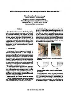
Computational Method for Segmentation and Classification of ...
Recommend Documents
Marketing Engineering for Excel is a Microsoft Excel add-in. The software runs
from within Microsoft Excel and only with data contained in an Excel spreadsheet.
term of greatest lower bound of a fuzzy assertion w.r.t. Σ was defined in [14]. ... In order to store the fuzzy knowledge base produced by FiRE in a Sesame.
more suitable method according to text characteristics. 1. Introduction. Text segmentation according to a topical criterion is a useful process in many applications ...
action between global classification and local region labels. ..... (World Rally Championship) has specializationOf as an RDF predicate and rally forms the RDF ...
Classification and reconstruction of archaeological frag- ments is based on the .... Then, it is possible to normalize these splines so that for any x ¾[a, b] n+3. Σ .... on Synthetic-Natural Hybrid Coding and Three Dimensional. Imaging, Santorini
Jan 20, 2017 - accessible via GitHub: The classification software ...... from the 1 μm diameter observed by scanning electron microscopy (SEM). This was ...
tions are individually mounted on glass microscope slides for staining and then scanned to produce virtual slides for scoring and annotation of phenotypes (see ...
are: (a) the number of zero crossings of the waveform in a 10 msec window .... the minimum zero crossing rate 30 msec before the peak was too high, (b) the ...
Results from test data demonstrate the method's robustness to analyze livers from ... the accurate classification of tum
fluor, (d) Red fluor, (e) Gold fluor and (f) Color M-FISH image. In this study region based segmentation and classification is proposed as a two-stage process.
Jun 11, 2008 - Arnaud Martina, Hicham Laanayaab and Andreas Arnold-Bosa. aENSIETA E3I2 EA3876,. 2 rue François Verny, 29806 Brest Cedex 09, France.
segmentation map and the distribution mixture parameters are then ..... TAB. 1: Estimated parameters for the picture reported in Fig. 2. stands for the proportion ...
Figure 2: People identified by the CAMEO system's face detector. We have implemented the PowerPoint Scraper that uses the Mi- crosoft PowerPoint API to ...
Heart Failure Etiology Based on Gene Expression Data. HY Wang, H Zheng, ... least squares, nearest shrunken centroids and random forests, showed similar ...
... Radiology Laboratory, Chil- dren's Hospital, Harvard Medical School, Boston, MA 02115 USA (e-mail: ... Color versions of one or more of the figures in this paper are available online ..... films as reference, one trained technician outlined the c
School of Eng. and Computer Science, Hebrew University of Jerusalem, Israel. 2. Sourasky ... compared to manual segmentation by an expert radiologist.
with good precision using combinations of widely-used image processing .... tree, which represents the full data set, the best degree of discrimination (or âbest.
Abstract. Multiplex Fluorescent In Situ Hybridization (M-FISH) is a newly chromosome imaging technique where each chromosome class appears to have a ...
CLUTTERED SCENES â AN INTEGRATED APPROACH. Stefan Müller, Stefan Eickeler, Christoph Neukirchen, Bernd Winterstein. Department of Computer ...
determines the pathos condition in the blood which shows WBC plays a vital factor in blood count. Normally white blood corpuscles count ranges from.
objects correspond to segments that occur in di erent levels of a segmentation pyramid. A set of segments is selected from the pyramid by classifying each ...
Aug 3, 2017 - Madamira: A fast, comprehensive tool for morphological analysis and disambiguation of Ara- bic. Proc. LREC . Maria Persson. 2008. The role of ...
The first part evaluates the statistical reliability of human ... a use of a sen- tence or other linguistic unit, whether in text or spoken language. ... erent of the underlined noun phrase a man with a goat is a .... phrases with sentence-final cont
word segmentation in Urdu not only has space omission ... being carried over to Urdu from English literate .... 1991) try to match longest possible dictionary.
Computational Method for Segmentation and Classification of ...
Oct 21, 2008 - Classification of Ingestive Sounds in Sheep. D. H. Milonea ..... In order to construct the pasture independent model (Mind) we followed a. 238. 2.
sinc(i) Research Center for Signals, Systems and Computational Intelligence (fich.unl.edu.ar/sinc) D.H. Milone, H.L. Rufiner, J.R. Galli, E.A. Laca & C.A. Cangiano; "Computational method for segmentation and classification of ingestive sounds in sheep" Computers and Electronics in Agriculture, Vol. 65, No. 2, pp. 228 - 237, 2009.
Computational Method for Segmentation and Classification of Ingestive Sounds in Sheep
D. H. Milone a,b,∗ , H. L. Rufiner a,b,d , J. R. Galli c , E. A. Laca f , C. A. Cangiano e a Laboratorio
de Se˜ nales e Inteligencia Computacional.
Facultad de Ingenier´ıa y Cs. H´ıdricas, Universidad Nacional del Litoral CC 217, Ciudad Universitaria, Paraje El Pozo, S3000 Santa Fe, Argentina b Consejo
Nacional de Investigaciones Cient´ıficas y T´ecnicas, Argentina
c Facultad d Lab.
de Cs. Agrarias, Univ. Nacional de Rosario, Argentina
de Cibern´etica, Fac. de Ingenier´ıa, Univ. Nac. de Entre R´ıos, Argentina
e EEA
Balcarce, Instituto Nacional de Tecnolog´ıa Agropecuaria, Argentina f Department
of Plant Science, Univ. of California, Davis
Preprint submitted to Comp. and Elect. in Agriculture
October 21, 2008
sinc(i) Research Center for Signals, Systems and Computational Intelligence (fich.unl.edu.ar/sinc) D.H. Milone, H.L. Rufiner, J.R. Galli, E.A. Laca & C.A. Cangiano; "Computational method for segmentation and classification of ingestive sounds in sheep" Computers and Electronics in Agriculture, Vol. 65, No. 2, pp. 228 - 237, 2009.
1
Abstract
2
In this work we propose a novel method to analyze and recognize automatically
3
sound signals of chewing and biting. For the automatic segmentation and classi-
4
fication of acoustical ingestive behaviour of sheep the method use an appropriate
5
acoustic representation and statistical modelling based on hidden Markov models.
6
We analyzed 1813 seconds of chewing data from four sheep eating two different for-
7
ages typically found in grazing production systems, orchardgrass and alfalfa, each
8
at two sward heights. Because identification of species consumed when in mixed
9
swards is a key issue in grazing science, we tested the possibility to discriminate
10
species and sward height by using the proposed approach. Signals were correctly
11
classified by forage and sward height in 67% of the cases, whereas forage was cor-
12
rectly identified 84% of the time. The results showed an overall performance of 82%
13
for the recognition of chewing events.
14
Key words:
15
behaviour.
16
1
17
Accurate measurement of feeding behavior are essential for a reliable manage-
18
ment and investigation of grazing ruminants. An indication of animal health
19
and welfare can be obtained by monitoring grazing and rumination activities,
20
because ruminants have a daily chewing requirement to maintain a healthy
∗ Corresponding author. Email address: [email protected] (D. H. Milone).
2
sinc(i) Research Center for Signals, Systems and Computational Intelligence (fich.unl.edu.ar/sinc) D.H. Milone, H.L. Rufiner, J.R. Galli, E.A. Laca & C.A. Cangiano; "Computational method for segmentation and classification of ingestive sounds in sheep" Computers and Electronics in Agriculture, Vol. 65, No. 2, pp. 228 - 237, 2009.
22
Grazing ruminants spend a large part of their lives biting (grasping and sev-
23
ering the herbage in the field) and chewing (grinding of the herbage inside
24
the mouth). They expend quite a lot of energy in eating behavior. When con-
25
suming high quality roughage, roughly 10% of the energy content of the feed
26
is consumed in the eating process. On low quality feed, such as wheat straw,
27
that figure jumps to about 25% of energy content (Susenbeth et al., 1998).
28
Other methods for chewing behavior studies rely on direct observation or on
29
the use of switches and jaw strap adjustment (Stobbs and Cowper, 1972; Pen-
30
ning, 1983; Matsui and Okubo, 1991; Rutter et al., 1997). Direct observation
31
is costly and frequently infeasible. Both direct observation and methods based
32
on jaw movements cannot detect the overlap between chewing and biting.
33
Acoustic biotelemetry has been proposed for animal behavior studies because
34
of the rich information contained in sounds (Alkon et al., 1989) and because
35
sound can be recorded and collected without affecting animal behaviour (Laca
36
et al., 1992; Klein et al., 1994; Nelson et al., 2005).
37
Acoustic analysis has been proved useful to discriminate a combined chew-bite
38
during a single jaw movement (Laca et al., 1994), to identify some spectral
39
differences of biting and chewing in cattle and it was shown to be a promis-
40
ing method to estimate voluntary intake in different types of feed (Laca and
41
Wallis DeVries, 2000; Galli et al., 2006).
42
Nevertheless, this method requires further research and development to doc-
43
ument the potential of acoustic monitoring of ingestive behavior of animals
44
to yield a consistent automatic decoding of chewing sounds in a variety of
45
conditions. Although discrimination of eating (Nelson et al., 2005; Ungar and
46
Rutter, 2006) and ruminating (Cangiano et al., 2006) sounds appears to be 3
sinc(i) Research Center for Signals, Systems and Computational Intelligence (fich.unl.edu.ar/sinc) D.H. Milone, H.L. Rufiner, J.R. Galli, E.A. Laca & C.A. Cangiano; "Computational method for segmentation and classification of ingestive sounds in sheep" Computers and Electronics in Agriculture, Vol. 65, No. 2, pp. 228 - 237, 2009.
47
accurate, in the past, sound records have been analyzed manually which is
48
an arduous task. A system for automatic processing and recognition of sound
49
signals is needed to refine and speed up the method.
50
Automatic speech recognition (ASR) has been an active field of research in
51
the past two decades (Huang et al., 2001). The main blocks of a speech recog-
52
nizer are: speech signal analysis, acoustic and language modeling. Statistical
53
methods such as hidden Markov models (HMM) have performed well in ASR
54
(Rabiner and Juang, 1986). It is likely that the methods and technologies de-
55
veloped for ASR will be applicable to the analysis of sounds produced by the
56
ingestive behaviour of ruminants. Recently, this type of tools has been used
57
to study and characterize vocal sounds generated by vocalizations of other
58
animals such as red deer (Reby et al., 2006). The objective of our research
59
was to propose a novel method, based on an appropriate signal representation
60
and HMM, to allow the automatic segmentation and classification of bites and
61
chews in sheep grazing a variety of pastures.
62
The general structure of the proposed system resembles to that of a speech
63
recognition system, where phoneme models are replaced by masticatory sub-
64
events and word models by complete events (such as a chew, bite or combined
65
chew-bite event). As in the speech case, the language model (LM) captures
66
the long-term dependencies and constrains the possible sequences.
67
This paper was organized as follows. In the next section a brief introduction
68
to hidden Markov models is provided. In Section 3, the sound registration
69
procedure and the data employed for the experiments are presented. Then
70
the statistical model of the acoustic signal is developed and the measures for
71
evaluating its performance were presented. Next, the results of the proposed 4
sinc(i) Research Center for Signals, Systems and Computational Intelligence (fich.unl.edu.ar/sinc) D.H. Milone, H.L. Rufiner, J.R. Galli, E.A. Laca & C.A. Cangiano; "Computational method for segmentation and classification of ingestive sounds in sheep" Computers and Electronics in Agriculture, Vol. 65, No. 2, pp. 228 - 237, 2009.
Figure 1. A discrete hidden Markov model with 2 states and 3 output symbols: aij are the transition probabilities and bi (k) is the probability of emitting the symbol ok in state i. 72
experiments are presented and discussed. Finally the conclusions and sugges-
73
tions for future work are posed.
74
2
75
In this section we will introduce the main concepts behind hidden Markov
76
models, through a simple numerical example. Suppose we want to model se-
77
quences of discrete symbols X = x1 , x2 , . . . xT , where xt ∈ O, the set of possible
78
symbols, and t ∈ N stands for the time order in the sequence. For example,
79
with the symbols set O = { , ⊕, } we can think of the graph of Figure 1
80
as a generative model for sequences like X. This is an instance of a discrete
81
hidden Markov model (DHMM), with only 2 states (Q = {1, 2}), and the 3
82
symbols as the possible outputs. In a Markov chain, given present state qt , the
83
next state qt+1 is independent of the past states qt−1 , qt−2 , . . . , q1 . Therefore,
84
the transitions between states can be defined with the matrix of probabil-
85
ities A = [aij = Pr (qt+1 = j|qt = i)], where i, j ∈ Q. For the generation of
86
sequences, each state i is related to the symbols ok by an emission distribu-
87
tion bi (k) = Pr (x = ok |q = i). Using all these components, the DHMM can be
88
defined with the structure Θ = {O, Q, A, B}.
Hidden Markov models
5
89
Consider the model Θ with the following probabilities:
sinc(i) Research Center for Signals, Systems and Computational Intelligence (fich.unl.edu.ar/sinc) D.H. Milone, H.L. Rufiner, J.R. Galli, E.A. Laca & C.A. Cangiano; "Computational method for segmentation and classification of ingestive sounds in sheep" Computers and Electronics in Agriculture, Vol. 65, No. 2, pp. 228 - 237, 2009.
A=
9 1 10 10
B=
0 1
1 1 4 10 10 5 9 1 1
,
10 20 20
90
where B is the emissions matrix, that specifies the probability of observing
91
each symbol in the actual state. Given the output sequence X = ⊕, , , , we
92
now ask for the probability of X given that the model is fully specified. Since
93
we do not know the sequence of states that generated this output sequence,
94
we say that the model is hidden, and the states are often referred as latent
95
variables of the model. Thus, to compute the probability of X given the model
96
Θ, we need to consider all the possible sequences of states and sum up over
97
all the cases (that is, the total probability formula).
98
The model in Figure 1 is known as a left-to-right HMM, because there are only
99
forward links and self loops (notice that a21 = 0). In this example, the first
100
state in a sequence will always be the state 1, known as initial state. Similarly,
101
state 2 is the terminal state and all the sequences of states should end with
102
this state. Thus, once the terminal state is reached, the model must observe
103
all the remaining symbols in the same state (that is, a22 = 1). For a sequence
104
of four symbols, all the possible sequences of states are: q1 = 1→1→1→2,
105
q2 = 1→1→2→2, and q3 = 1→2→2→2. In the first sequence of transitions we
106
have: the emission of symbol ⊕ in state q1 = 1, b1 (2) =
107
the first state to itself at time 2, a11 =
108
the second transition a11 =
109
transition, now from state 1 to state 2, a12 =
9 ; 10
9 ; 10
1 ; 10
the transition from
the emission of symbol , b1 (3) = 45 ;
the emission of symbol , b1 (1) =
6
1 ; 10
1 ; 10
the third
and the last emission, of
sinc(i) Research Center for Signals, Systems and Computational Intelligence (fich.unl.edu.ar/sinc) D.H. Milone, H.L. Rufiner, J.R. Galli, E.A. Laca & C.A. Cangiano; "Computational method for segmentation and classification of ingestive sounds in sheep" Computers and Electronics in Agriculture, Vol. 65, No. 2, pp. 228 - 237, 2009.
9 . 10
110
symbol in state q4 = 2, b2 (1) =
111
obtain Pr(X|q1 ) =
112
0.006 and Pr(X|q3 ) ≈ 0.0004. Then, the probability of the emission sequence
113
given the model is Pr(X) = Pr(X|q1 ) + Pr(X|q2 ) + Pr(X|q3 ) ≈ 0.007.
114
For the classification tasks we build an HMM for each event to be recognized
115
and then, given an emission sequence of unknown class, we classify it as that
116
corresponding to the most probable model. As it can be seen in the previous
117
example, the probability of the most probable sequence of states is a good
118
approximation to the total probability.
119
The training or parameter estimation problem remains unaddressed. That is,
120
given a set of sequences of emissions, we are looking for the model probabilities
121
A and B that best fit the data. An intuitive process can be: obtain the best
122
sequences of states for each sequence of emissions and then count the number of
123
transition between states. Thus, probabilities in A can be approximated by the
124
relative frequencies of transitions. In the same way, by counting the times that
125
each state emit a symbol, we can estimate the emission probabilities in B. This
126
algorithm is known as the forced-alignment training and it is based in the fast
127
algorithm proposed by Viterbi (1967). A more complete estimation that uses
128
all the sequences of states (weighted by its probabilities) can be done with the
129
Baum-Welch training method. The forward-backward algorithm provides an
130
efficient way to compute the probabilities for all the sequences and reestimates
131
the parameters in an acceptable processing time for real applications (Huang
132
et al., 1990).
133
In the case of the acoustic modeling, the sequences of symbols are indeed
134
sequences of spectra. Acoustic models of sounds have evolved from vector
1 9 4 9 1 1 9 10 10 5 10 10 10 10
By using all these probabilities we can
≈ 0.0006. Similarly, we get Pr(X|q2 ) ≈
7
sinc(i) Research Center for Signals, Systems and Computational Intelligence (fich.unl.edu.ar/sinc) D.H. Milone, H.L. Rufiner, J.R. Galli, E.A. Laca & C.A. Cangiano; "Computational method for segmentation and classification of ingestive sounds in sheep" Computers and Electronics in Agriculture, Vol. 65, No. 2, pp. 228 - 237, 2009.
135
quantization with DHMM to more direct models of spectral information with
136
continuous observation density hidden Markov models (CHMM). In the former
137
systems, acoustic features are mapped to a finite set of discrete elements, that
138
is, the outputs of a vector quantizer (Gray, 1984). Thus, it was possible to use
139
DHMM to model sequences of spectral representations. However, in CHMM
140
it is possible to model continuous observation densities in the HMM itself –
141
instead of vector quantization, taking advantage of modeling selected features
142
through Gaussian mixtures (Rabiner and Juang, 1993). To train these mod-
143
els, Liporace (1982) defined the auxiliary function to use in the expectation-
144
maximization (EM) algorithm. He proved that using Gaussian mixtures in the
145
HMM states, this auxiliary function has a unique global maximum as function
146
of the model parameters. The Baum-Welch training uses this EM algorithm
147
and can reach the global maximum given that, as proved in the same work,
148
the sequence of reestimates obtained in produce a monotonic increase in the
149
likelihood of the data given the model.
150
3
151
3.1
152
Acoustic signals were obtained from a grazing experiment performed at Uni-
153
versity of California, Davis. The experiment consisted of a factorial of two
154
forages and two plant heights grazed by sheep. The forages were orchardgrass
155
(Dactylis glomerata) and alfalfa (Medicago sativa) in a vegetative state. Al-
156
falfa and orchardgrass were offered in two plant heights, tall (not defoliated,
157
29.8 ± 0.79 cm) and short (clipped with scissors to approximately
Materials and methods
Sound registration
8
1/2
the
sinc(i) Research Center for Signals, Systems and Computational Intelligence (fich.unl.edu.ar/sinc) D.H. Milone, H.L. Rufiner, J.R. Galli, E.A. Laca & C.A. Cangiano; "Computational method for segmentation and classification of ingestive sounds in sheep" Computers and Electronics in Agriculture, Vol. 65, No. 2, pp. 228 - 237, 2009.
158
height of the tall treatment, 14.1 ± 0.79 cm). Pots were firmly attached to a
159
heavy wooden board that held them in place when grazed. We used four tame
160
crossbreed ewes that were 2-4 years old and weighed 85 ± 6.0 kg.
161
The order of all combinations of species, plant height and ewe was randomized,
162
and each day (between 12 and 16 h) 8-9 of these combinations (sessions) were
163
observed during six consecutive days. Randomization was restricted such that
164
each of the four combinations of species and plant height and the three ewes
165
were observed at least in one session each day. Animals were fed alfalfa hay
166
and spent the rest of the day in an adjacent yard.
167
Sounds were recorded using wireless microphones (Nady 155 VR, Nady Sys-
168
tems, Inc., Oakland, California) protected by a rubber foam and placed on
169
the animal’s forehead fastened to a halter where the transmitter was attached
170
(see Figure 2). Sound was recorded on the sound track of a digital camcorder.
171
A watch alarm was set to go off next to the microphone every 10 s as standard
172
sound. Recordings contain various types of natural environmental noises, like
173
bird songs. However, denoising was not applied, signals were fed to the recog-
174
nizer as recorded in natural environment. Sounds were originally digitized into
175
uncompressed PCM wave format, using a mono channel with a resolution of
176
16 bits at a sampling frequency of 44100 Hz. Due to the low-frequency nature
177
of signals they were re-sampled to 22050 Hz after processing by an appropriate
178
low-pass filter.
179
A preliminary comparison of the typical waveforms and spectrograms illus-
180
trates the differences between a chew, a bite and a chew-bite of grazing sheep.
181
Figure 3 shows the temporal sound wave and spectrogram of a sequence of
182
chews, bites and chew-bites of grazing sheep. Bites appear as a sequence of 9
sinc(i) Research Center for Signals, Systems and Computational Intelligence (fich.unl.edu.ar/sinc) D.H. Milone, H.L. Rufiner, J.R. Galli, E.A. Laca & C.A. Cangiano; "Computational method for segmentation and classification of ingestive sounds in sheep" Computers and Electronics in Agriculture, Vol. 65, No. 2, pp. 228 - 237, 2009.
Wireless microphone on animal’s forehead
Pots with plants attached to a wooden board
Figure 2. Schematic illustration of the experimental device for sound recording.
Figure 3. Sound wave (top) and narrow band spectrogram (bottom) of a sequence of chews, bites and chew-bites of grazing sheep. 183
short bursts of high frequency (Figure 4). Chewing has a relative high energy
184
in the lower half of the spectrum, sustained during a large proportion of its
185
duration (Figure 5). The chew-bite is a composite signal, relatively difficult to
186
be distinguished from the isolated chew signal (Figure 6). Sounds of all events
187
have non-stationary behaviour and their relative frequency contents overlap.
188
The corpus was formed by the original sound recordings of sheep grazing
189
short alfalfa, tall alfalfa, short orchardgrass and tall orchardgrass. Chews, 10
sinc(i) Research Center for Signals, Systems and Computational Intelligence (fich.unl.edu.ar/sinc) D.H. Milone, H.L. Rufiner, J.R. Galli, E.A. Laca & C.A. Cangiano; "Computational method for segmentation and classification of ingestive sounds in sheep" Computers and Electronics in Agriculture, Vol. 65, No. 2, pp. 228 - 237, 2009.
Figure 4. Sound wave (top) and narrow spectrogram (bottom) of an artificially isolated bite of grazing sheep.
Figure 5. Sound wave (top) and narrow band spectrogram (bottom) of an artificially isolated chew of grazing sheep. 190
bites and chew-bites were identified and labeled by animal behaviour experts
191
through direct vieweing and listening of the video files. The total lengths of
192
the registered sound data base were 563 and 457 seconds for tall and short 11
sinc(i) Research Center for Signals, Systems and Computational Intelligence (fich.unl.edu.ar/sinc) D.H. Milone, H.L. Rufiner, J.R. Galli, E.A. Laca & C.A. Cangiano; "Computational method for segmentation and classification of ingestive sounds in sheep" Computers and Electronics in Agriculture, Vol. 65, No. 2, pp. 228 - 237, 2009.
Figure 6. Sound wave (top) and narrow band spectrogram (bottom) of an artificially isolated chew-bite of grazing sheep. 193
alfalfa and 420 and 373 seconds for tall and short orchardgrass.
194
3.2
195
Signal preprocessing consisted of a preemphasis filter and mean subtraction.
196
Because of the non-stationarity of the signal, the next step is to apply short-
197
time analysis techniques. This type of analysis consists in split the whole
198
signal record in short segments called frames (Cohen, 1995). These frames are
199
extracted with some periodicity named step and have a characteristic time
200
width. If the frame width is greater than the step, two consecutive frames will
201
share some samples from the signal record. Each frame was smoothed with a
202
Hamming window to avoid the border effects of the splitting process, and then
203
it was analyzed with several standard spectral estimation techniques, such
204
as: linear prediction coefficients (LPC), linearly spanned filter-bank (FB), log
205
spanned FB, mel FB, cepstrum and mel cepstrum (Oppenheim and Schafer,
Signal analysis and recognition model
12
sinc(i) Research Center for Signals, Systems and Computational Intelligence (fich.unl.edu.ar/sinc) D.H. Milone, H.L. Rufiner, J.R. Galli, E.A. Laca & C.A. Cangiano; "Computational method for segmentation and classification of ingestive sounds in sheep" Computers and Electronics in Agriculture, Vol. 65, No. 2, pp. 228 - 237, 2009.
206
1989).
207
In the recognition model design, each event (bite, chew and chew-bite) was
208
modeled as a concatenation of sub-events (bite = [b1 ,→ b2], chew = [c1 ,→
209
c2 ,→ c3] and chew-bite= [cb1 ,→ cb2 ,→ cb3]) and, each sub-event as an HMM.
210
Also, one sub-event could have several states and each state could observe one
211
or more frames. The silence was also modeled as a sil event 1 . Finally, the
212
individual event models were associated by a language model (LM) into a
213
compound model for every possible sequence of events.
214
In Fig. 7 we can see the compound model used for the recognition experiments
215
(expanded with more detail for the event chew). Each HMM has its states,
216
transition probabilities and probability density functions for the emissions.
217
In our case, gaussian mixtures were used at each state to model the spectral
218
features (i.e., CHMM). We used the above mentioned Baum-Welch algorithm
219
in order to train the HMM transition and observation probabilities.
220
The LM allows concatenating large sequences of events to model the whole
221
signal record (in a statistical way). In a simple bigram LM, the a priori prob-
222
ability that an event occurs given a previous event is used (Jelinek, 1999).
223
For example, a bite is frequently followed by a chew, thus, the probability
224
for the sequence [bite chew] is greater than the probability for the sequence
225
[bite bite]. In the same sense the probability for the sequence [chew chew]
226
would be greater than the probability for the sequence [chew bite]. Figure 8
227
shows the general bigram LM used in this work.
228
Once trained, we used the model to recognize unknown sounds by means of
229
standard Viterbi algorithm (Rabiner and Juang, 1993). All the experiments 1
In some experiments the sil event was modeled as a sub-event of the others events.
13
s1
s2
s3
s1
s2
s3
s1
s2
s3
sinc(i) Research Center for Signals, Systems and Computational Intelligence (fich.unl.edu.ar/sinc) D.H. Milone, H.L. Rufiner, J.R. Galli, E.A. Laca & C.A. Cangiano; "Computational method for segmentation and classification of ingestive sounds in sheep" Computers and Electronics in Agriculture, Vol. 65, No. 2, pp. 228 - 237, 2009.
Acoustic level
Sub-event level
c1
Event level
c2
chew
c3
chew-bite
bite
Compound level
sil
Language model
Figure 7. Schematic diagram of the compound model used for the recognition experiments. The different states represent the events at the acoustic level, while individual HMMs have been used to represent the sub-event level. Each sub-event model was merge into an event model by a dictionary and all this events are associated in a compound model by a language model.
bite S
sil
chew
sil
E
chew-bite
Figure 8. General language model used for the experiments. S means “start” and E means “end”. 230
were implemented using the HTK toolkit 2 . The configuration details will be
231
given in the next section.
232
The before mentioned compound model was used for the experiments with
233
only one species and height of pasture. In this case the model had three possible
234
output classes of events for the sequence (bite, chew and chew-bite). It was
235
a pasture dependent model (for one species and one height). Four different
236
pasture dependent models were trained: tall alfalfa (MT A ), short alfalfa (MSA ),
237
tall orchardgras (MT O ) and short orchardgrass (MSO ).
238
In order to construct the pasture independent model (Mind ) we followed a 2
http://htk.eng.cam.ac.uk
14
sinc(i) Research Center for Signals, Systems and Computational Intelligence (fich.unl.edu.ar/sinc) D.H. Milone, H.L. Rufiner, J.R. Galli, E.A. Laca & C.A. Cangiano; "Computational method for segmentation and classification of ingestive sounds in sheep" Computers and Electronics in Agriculture, Vol. 65, No. 2, pp. 228 - 237, 2009.
239
similar way but using twelve events classes (and silence): one bite, chew and
240
chew-bite different model for every one of each four pasture conditions. For
241
example for tall alfalfa we had biteT A , chewT A and chew-bite T A events, for
242
short alfalfa we had biteSA , chewSA events and chew-bite SA , and so on. All
243
these events were associated in an overall model, extending the LM to include
244
12 events.
245
3.3
246
In order to achieve statistically representative results, all the tests were con-
247
ducted according to the averaged leave-k-out method (Michie et al., 1994).
248
The complete data set was randomly split 10 times in train/test sets, using
249
the 80% of total signals for training and the remaining 20% for recognition.
Recognition performance measures
For each test partition, the performance was evaluated by using the recognition rate and the recognition accuracy, respectively as follows: N Pj
Cj =
N Pj
Tji − Dji − Sji
i=1 N Pj
Aj =
Tji − Dji − Sji − Iji
i=1
Tji
i=1
N Pj
Tji
i=1
250
where:
251
Nj : total number of sequences in test partition j
252
Tji : total number of events in the sequence i of the test partition j
253
Dji : deleted events in the recognized sequences i of the test partition j
254
Sji : substituted events in the recognized sequences i of the test partition j
255
Iji : inserted events in the recognized sequences i of the test partition j
256
15
sinc(i) Research Center for Signals, Systems and Computational Intelligence (fich.unl.edu.ar/sinc) D.H. Milone, H.L. Rufiner, J.R. Galli, E.A. Laca & C.A. Cangiano; "Computational method for segmentation and classification of ingestive sounds in sheep" Computers and Electronics in Agriculture, Vol. 65, No. 2, pp. 228 - 237, 2009.
257
In all the counts, silence events are ignored and the final results are computed
258
as the average among all test partitions. To obtain the Dji , Sji and Iji counts,
259
a dynamic programming alignment between the hand labeled reference se-
260
quence (Refseq ) and the recognized sequence (Recseq ) was performed (Young
261
et al., 2000). An example of the recognizer output is reproduced here with the
262
corresponding hand-labeled reference: Refseq :
[ bite
chew
chew
Recseq :
[ bite
chew
chew
chew
chew
bite
chew
chew
chew
chew
chew
chew
]
263
bite
]
264
The second bite from the recognized sequence is an insertion and the fifth
265
chew is a substitution. The last event from the reference sequence has not
266
been recognized so it is a deletion. From this example it can be seen that Aj
267
is a much more exigent measure since it considers insertions while Cj does
268
not. Aj is very useful to make decisions about the overall system performance,
269
because if Iji is greater than Tji , Cj can be high (near 100%) while Aj will
270
be negative. However, once a system has reached a reasonable Aj (say, 80%)
271
then Cj can be used to select the best system configuration.
272
We also used the confusion matrix as another method to evaluate classification
273
performance. In confusion matrices, each column represents a predicted event
274
class, while each row represents the actual class. One benefit of a confusion
275
matrix is that it is easy to see if the system is confusing two classes.
276
4
277
For the feature extraction the best recognition rates among parametric tech-
278
niques were for LPC. For non-parametric techniques best results were for
Experiments and Results
16
sinc(i) Research Center for Signals, Systems and Computational Intelligence (fich.unl.edu.ar/sinc) D.H. Milone, H.L. Rufiner, J.R. Galli, E.A. Laca & C.A. Cangiano; "Computational method for segmentation and classification of ingestive sounds in sheep" Computers and Electronics in Agriculture, Vol. 65, No. 2, pp. 228 - 237, 2009.
279
linearly spanned FB. We employed 10 linearly spanned bands between 0 and
280
2000 Hz for the FB and 20 coefficients for LPC. In addition, an estimation of
281
the derivatives and total energy in the spectral estimation was used. Frame
282
width ranged from 10 ms to 100 ms in steps of 10 ms and overlapping ranged
283
from 0% to 75% in steps of 25%. Best results were obtained with a frame
284
width of 20 ms and an overlapping of 25%.
285
In the tuning of the HMM architecture, we first made tests using one model per
286
event, where the number of emitting states ranged from 2 to 8. These results
287
were useful as a baseline for the following stage. Based on visual inspection of
288
the sound signal, chews and chew-bites were modeled by three sub-events, bites
289
with two and silence with only one. This division in sub-events is justified by
290
the different spectral evolution between ingestive events but not for the silence
291
that should remain almost stationary.
292
Using the Gaussian means of the trained models, one can build the estimated
293
spectra that HMM holds in each state. This could provide some insights about
294
the internal model representation of spectral signal dynamics, remarking the
295
important characteristics that it takes into account. As an example we used
296
the MT A trained. The spectral dynamic for bite is modeled by two sub-events
297
(b1 and b2) each with three states (Figure 9). Chew is modeled by three sub-
298
events (c1, c2 and c3) each with three states (Figure 10). Chew-bite is also
299
modeled by three sub-events (cb1, cb2 and cb3) each with three states (Figure
300
11). Bite spectra for the first state of b1 has an important peak around 1
301
kHz, alternating between narrow and broad-band spectra for the rest of the
302
states. It also finishes the last state of b2 with a peaked spectrum again. If
303
we carefully inspect Figure 4, this is compatible with the sequence of short
304
duration bursts (naturally broad-band) and low energy regions (which presents 17
sinc(i) Research Center for Signals, Systems and Computational Intelligence (fich.unl.edu.ar/sinc) D.H. Milone, H.L. Rufiner, J.R. Galli, E.A. Laca & C.A. Cangiano; "Computational method for segmentation and classification of ingestive sounds in sheep" Computers and Electronics in Agriculture, Vol. 65, No. 2, pp. 228 - 237, 2009.
log energy
b1 state1
b2 state1
0
0
-10
-10
-20
-20
-30
-30
log energy
b1 state2
b2 state2
0
0
-10
-10
-20
-20
-30
-30 0
5
log energy
b1 state3 0
0
-10
-10
-20
-20
-30 0
10
b2 state3
5 10 frequency [kHz]
-30 0
5 10 frequency [kHz]
Figure 9. Spectra of bite estimated by the tall alfalfa model after the training process, computed from the Gaussian means of LPC parameters of each model state. Columns: sub-events; Rows: states.
log energy
c1 state1
c2 state1 0
0
-10
-10
-10
-20
-20
-20
-30
-30
-30
log energy
c1 state2
c2 state2
c3 state2
0
0
0
-10
-10
-10
-20
-20
-20
-30
-30
-30
c1 state3 log energy
c3 state1
0
c2 state3
c3 state3
0
0
0
-10
-10
-10
-20
-20
-20
-30 0
5 10 frequency [kHz]
-30 0
5 10 frequency [kHz]
-30 0
5 10 frequency [kHz]
Figure 10. Spectra of chew estimated by the tall alfalfa model after the training process, computed from the Gaussian means of LPC parameters of each model state. Columns: sub-events; Rows: states. 305
relative concentration of energy around 1 kHz) displayed in it. Chew spectra
306
varies from one with a relative flatness for c1 to one more concentrated around
307
the bottom half in c2, finishing with spectra in c3 similar to c1 (but in reverse 18
cb2 state1
log energy
cb3 state1
0
0
-10
-10
-10
-20
-20
-20
-30
-30
-30
cb1 state2
cb2 state2
cb3 state2
0
0
0
-10
-10
-10
-20
-20
-20
-30
-30
-30
cb1 state3 log energy
sinc(i) Research Center for Signals, Systems and Computational Intelligence (fich.unl.edu.ar/sinc) D.H. Milone, H.L. Rufiner, J.R. Galli, E.A. Laca & C.A. Cangiano; "Computational method for segmentation and classification of ingestive sounds in sheep" Computers and Electronics in Agriculture, Vol. 65, No. 2, pp. 228 - 237, 2009.
log energy
cb1 state1 0
cb2 state3
cb3 state3
0
0
0
-10
-10
-10
-20
-20
-20
-30 0
5 10 frequency [kHz]
-30 0
5 10 frequency [kHz]
-30 0
5 10 frequency [kHz]
Figure 11. Spectra of chew-bite estimated by the tall alfalfa model after the training process, computed from the Gaussian means of LPC parameters of each model state. Columns: sub-events; Rows: states. 308
order). This is clearly related with the example of chew presented in Figure
309
5. As expected, spectrum of the first sub-events of chew-bite were similar to
310
those of chew while the last (cb3 state 3, Figure 11) was similar to those of
311
bite. This is associated with the composite signal nature observed in Figure
312
6.
313
Our preliminary results (not shown here for brevity) revealed that, for all the
314
cases, the models that used LPC as parameterization performed better than
315
those that used FB. Also, the use of more than one model per event obtained
316
higher recognition rates, compared to the baseline of one model per event.
317
After extensive trials, the best recognition results were obtained with a window
318
of 20 ms and an overlapping 15 ms, using 3 emitting states per HMM. In this
319
case, the system yielded an average Aj of 81.60% and an average Cj of 89.47%.
320
This analysis was carried out using the tall alfalfa files and MT A model, and
321
it set the basic system configuration that was employed afterwards. 19
sinc(i) Research Center for Signals, Systems and Computational Intelligence (fich.unl.edu.ar/sinc) D.H. Milone, H.L. Rufiner, J.R. Galli, E.A. Laca & C.A. Cangiano; "Computational method for segmentation and classification of ingestive sounds in sheep" Computers and Electronics in Agriculture, Vol. 65, No. 2, pp. 228 - 237, 2009.
Table 1 Recognition results classifying pasture species and height, by relabeling Mind model (see details in text).
Average Aj (%)
Average Cj (%)
dir−sil Mind species and height
51.59
58.11
sub−sil Mind species and height
61.63
66.53
sub−sil Mind species only
80.54
83.78
322
We will first present the detailed results of the pasture independent model
323
Mind . In this case we employed the previous described configuration and the
324
extended LM for 12 events. We used two different models for these exper-
325
dir−sil iments: modelling the sil event directly (Mind ) or as a sub-event of the
As explained before, the model was trained with the different pastures condi-
328
tions.
329
The grazing behaviour and diet selection by sheep are influenced by the sward
330
height and the relative species content of pastures (Illius et al., 1992). Conse-
331
quently it would be useful for reseachers to obtain an accurate classification of
332
ingestive sounds for different species and different heights within species. In or-
333
der to obtain different recognition results once trained we re-labelled the final
334
classes or events in the model. The first case was for the recognition of species
335
and height of pasture, that is a four classes problem. For example for tall alfalfa
336
class we replace biteT A → T A, chewT A → T A and chew-bite T A → T A. The
337
second required result was the recognition of species only, that is a two classes
338
problem. For example for alfalfa class we replace biteT A → A, chewT A → A,
339
chew-bite T A → A, biteSA → A, chewSA → A and chew-bite SA → A. The
340
results for this problems are shown in Table 1. When dealing with mixtures of
341
pastures, the system turned on recognizing the species and height of pasture
342
with a performance of 66.53%, while on the recognition of only the species the 20
sinc(i) Research Center for Signals, Systems and Computational Intelligence (fich.unl.edu.ar/sinc) D.H. Milone, H.L. Rufiner, J.R. Galli, E.A. Laca & C.A. Cangiano; "Computational method for segmentation and classification of ingestive sounds in sheep" Computers and Electronics in Agriculture, Vol. 65, No. 2, pp. 228 - 237, 2009.
Table 2 Confusion matrix for classifying bites, chews and chew-bites, by relabeling Mind model (values in parenthesis are %). bite’s
chew’s
chew-bite’s
bite’s
438 (58)
160 (21)
154 (21)
chew’s
182 (4)
4658 (89)
380 (7)
chew-bite’s
90 (13)
222 (31)
402 (56)
343
result grew up to 83.78%.
344
sub−sil Another case is to use Mind to recognize the event without taking into
345
account the pasture conditions (i.e. for bite class we replace biteT A → bite,
346
biteSA → bite, biteT O → bite and biteSO → bite). The results are displayed
347
in Table 2. Overall classification performance of events was 82%, where we
348
obtained 58% for bites, 89% for chews and 56% for chew-bites (see confusion
349
matrix diagonal, Table 2). Chews were classified as chew-bites in 7% of the
350
cases, chew-bites were partially misclassified as bites in 13% and chews in 31%.
351
In the pasture dependent models, where only one species and height were
352
considered, recognition values were generally higher than the previous ones.
353
The results for tall alfalfa MTsub−sil were 74, 96 and 61% of bites, chews and A
354
sub−sil chew-bites, respectively. Similar results were obtained for short alfalfa MSA
355
(68, 94 and 49 %). Tall orchardgrass MTsub−sil resulted in 66, 90 and 39% and O
356
sub−sil short orchardgrass MSO performed slighty worse with 18, 77 and 74%,
357
probably due to a relative lower signal to noise ratio for this type of sounds.
358
5
359
To our knowledge this is the first time an automatic recognition of ingestive
360
chewing of ruminants is done and it extends the use of HMM beyond vocal-
Discussion
21
sinc(i) Research Center for Signals, Systems and Computational Intelligence (fich.unl.edu.ar/sinc) D.H. Milone, H.L. Rufiner, J.R. Galli, E.A. Laca & C.A. Cangiano; "Computational method for segmentation and classification of ingestive sounds in sheep" Computers and Electronics in Agriculture, Vol. 65, No. 2, pp. 228 - 237, 2009.
361
izations studies in wild animals (Clemins et al., 2005; Reby et al., 2006).
362
The systems was effective and robust for the automatic segmentation and
363
classification of chewing behaviour in sheep. It speed-up the processing of
364
data and leaving the real time factor from hours to minutes, including the
365
analysis of other useful variables such as energy of chews (Galli et al., 2006)
366
while (Laca and Wallis DeVries, 2000) took nearly of 120 hours to manage
367
nearly 1000 bites and chews of steers.
368
The individual recognition models for each species have better performance
369
than using a unique overall model. These last ones had a high error rate mainly
370
because of event substitution. Nevertheless, they could be useful for prelimi-
371
nary segmentation of signals with unknown species and height of pasture.
372
The values obtained for window width and overlapping are indicators of the
373
signal stationarity, in the sense that its spectral characteristics (LPC or the
374
spectrum itself) do not show significant variation in the interval, so one frame
375
can be distinguished from another using a spectral distance measure. The
376
3-state models have demonstrated to be sufficient to model human speech
377
phonemes, so we consider reasonable that best results have been obtained
378
with models of few states. Carefully inspection of Figures 9, 10 and 11 seems
379
to indicate that the proposed number of states and sub-events allows the model
380
to correct follow the spectral dynamic of the events. A priori, chewing sounds
381
do not exhibit the complexity of speech, at least when considering the sound
382
generation mechanisms and the information content of both signals.
383
The surrounding noise such as animal vocalization and scratching against the
384
ground are difficult to filter out automatically. The overall system performance
385
is being altered because this sounds are generally classified as masticatory 22
sinc(i) Research Center for Signals, Systems and Computational Intelligence (fich.unl.edu.ar/sinc) D.H. Milone, H.L. Rufiner, J.R. Galli, E.A. Laca & C.A. Cangiano; "Computational method for segmentation and classification of ingestive sounds in sheep" Computers and Electronics in Agriculture, Vol. 65, No. 2, pp. 228 - 237, 2009.
386
events (they are not strictly silence) and this yields an error by insertion.
387
However, these sounds can be discarded by a previous stage because in gen-
388
eral are of short duration and low energy compared to those of the masticatory
389
events. Studies to determine if these sounds are very frequent must be made,
390
and a model for these events could be added to the system in order to im-
391
prove the general performance. This fact does not imply a major deviation in
392
the overall signal energy thus does not represent a problem when using the
393
chew energy for dry matter intake prediction (Laca and Wallis DeVries, 2000;
394
Galli et al., 2006). However, they represent an error when analyzing grazing
395
behaviour because they introduce a bias in the chews per bite ratio. Several
396
denoising techniques are also available, which could be used to improve signal
397
quality previously the starting of the recognition process.
398
The compound jaw movements, namely chew-bites and already detected in
399
cattle by Laca and Wallis DeVries (2000) were acoustically confirmed in sheep
400
and their spectra automatically recognized by trained HMM.
401
Since much of the acoustic signal generated by mechanical interaction of teeth
402
and food during occlusion is transmitted by bone conduction, the direct at-
403
tachment of the microphone to the forehead of bovine (Laca et al., 1994) or
404
head of mule deer (Nelson et al., 2005) picks up a wider range of sound than a
405
free-standing (collar–mounted) microphone, and can more easily pick up the
406
vibrations associated with mastication. The location is unobtrusive and proven
407
acceptable in controlled applications but for grazing extensive conditions could
408
be exposed to serious damage. The ear canal is one another possible place to
409
locate the microphone as a more secure and insulated position as already
410
proved in human (Amft et al., 2005). Furthermore, our system can be used
411
for real-time monitoring, at short distances, with wireless microphones. For an 23
sinc(i) Research Center for Signals, Systems and Computational Intelligence (fich.unl.edu.ar/sinc) D.H. Milone, H.L. Rufiner, J.R. Galli, E.A. Laca & C.A. Cangiano; "Computational method for segmentation and classification of ingestive sounds in sheep" Computers and Electronics in Agriculture, Vol. 65, No. 2, pp. 228 - 237, 2009.
412
implementation in a wide area, we are planning to incorporate a transmission
413
system over the cellular network or to use a recording system for several days
414
and then to process the signals in an standard personal computer. Alterna-
415
tively, a digital signal processor may be integrated with the microphone in the
416
forehead of each animal, but this may be a quite expensive solution.
417
6
418
We conclude that the automatic segmentation and classification of mastica-
419
tory sounds by sheep is possible by modelling the acoustical signals with con-
420
tinuous hidden Markov models. Models were tuned for optimal performance
421
using a compound model with different levels of analysis, from the acous-
422
tic of sub-events to the long-term dependence given by the intake language
423
model. This study provides a basis for future work on the complete automa-
424
tion of recording, segmentation and classification of masticatory sounds for
425
intake and grazing animal behaviour studies and for a wide application of the
426
acoustical method.
427
The ultimate goal of a system that precisely and reliably determines the type
428
and amount of food that the animal consumed is far. However, considering the
429
rate at which new commercial technologies become available, and the develop-
430
ment and analysis of larger sound data-bases, we can visualize an automated
431
acoustic monitoring system for ingestive behaviour in ruminants.
432
The novel approach we used has potential to be used no only as a technique
433
to automatically record and classify ingestive sounds, but also as a new way
434
to describe ingestive behaviour and to relate it to animal and forage char-
Conclusions and future work
24
sinc(i) Research Center for Signals, Systems and Computational Intelligence (fich.unl.edu.ar/sinc) D.H. Milone, H.L. Rufiner, J.R. Galli, E.A. Laca & C.A. Cangiano; "Computational method for segmentation and classification of ingestive sounds in sheep" Computers and Electronics in Agriculture, Vol. 65, No. 2, pp. 228 - 237, 2009.
435
acteristics. We hypothesize that the parameters for the language models are
436
synthetic descriptors of ingestive behavior that have the ability to integrate
437
the characteristics of feeding bouts into a few numbers. These numbers, such
438
as transition probabilities between behaviors and components of events could
439
be used to gain insight in the ingestion process. Automatic acoustig moni-
440
toring of ingestive behaviours is also valuable to assess animal welfare in a
441
manner that cannot be achieved with other methods, not even by direct vi-
442
sual observation. Ruminants can chew and bite within a single jaw movement.
443
Thus, mechanical or visual methods cannot fully discriminate these events
444
into simple bites or chew-bites. Chewing is a fundamental behavior for the
445
maintenance of rumen function and animal well-being because it supplies the
446
rumen with saliva, enzymes and buffering compounds. Acoustic monitoring
447
provides the most accurate quantification of chewing, and could be developed
448
into a routine method to monitor animals such as dairy cows that are subject
449
to the stresses of extremely high productivity.
450
7
451
This work was carried out with the financial support of ANPCyT and UNL,
452
under Projects PICTO-UNL No 36214 and CAI+D No 012-72, and of INTA
453
under Project PNLEC No 1101. The authors would like to thank Fernando
454
Guerin for his collaboration in the visual inspection and labeling of sound
455
signals and for models scripts debugging.
Acknowledgements
25
sinc(i) Research Center for Signals, Systems and Computational Intelligence (fich.unl.edu.ar/sinc) D.H. Milone, H.L. Rufiner, J.R. Galli, E.A. Laca & C.A. Cangiano; "Computational method for segmentation and classification of ingestive sounds in sheep" Computers and Electronics in Agriculture, Vol. 65, No. 2, pp. 228 - 237, 2009.
456
References
457
Alkon, P., Cohen, Y., Jordan, P., 1989. Towards an acoustic biotelemetry
458
system for animal behaviour studies. J. Wildlife Manage 53, 658–662.
459
Amft, O., St¨ager, M., Lukowicz, P., Tr¨oster, G., 2005. Analysis of chewing
460
sounds for dietary monitoring. In: Proceedings of the 7th International Con-
461
ference on Ubiquitous Computing. Tokyo, Japan, pp. 56–72.
462
463
Cangiano, C., Galli, J., Laca, E., 2006. El uso del sonido en el an´alisis de la rumia. Visi´on Rural 62, 23–24.
464
Clemins, P., Johnson, M., Leon, K., Savage, A., 2005. Automatic classification
465
and speaker identification of african elephant (loxodonta africana) vocaliza-
466
tions. Journal of the Acoustical Society of America, 956–963.
467
468
Cohen, L., 1995. Time Frequency Analysis: Theory and Applications. PrenticeHall.
469
Galli, J., Cangiano, C., Demment, M., Laca, E., 2006. Acoustic monitoring of
470
chewing and intake of fresh and dry forages in steers. Animal Feed Science
471
and Technology 128, 14–30.
472
473
Gray, R., 1984. Vector quantization. IEEE Acoustics Speech and Signal Processing Magazine 4, 4–29.
474
Huang, X., Acero, A., Hon, H.-W., May 2001. Spoken Language Processing: A
475
Guide to Theory, Algorithm and System Development. Prentice Hall PTR.
476
Huang, X. D., Ariki, Y., Jack, M. A., 1990. Hidden Markov Models for Speech
477
Recognition. Edinburgh University Press.
478
Illius, A. W., Clark, D. A., Hodgson, J., 1992. Discrimination and patch choice
479
by sheep grazing grass-clover swards. Journal of Animal Ecology 61, 183–
480
194.
481
Jelinek, F., 1999. Statistical Methods for Speech Recognition. MIT Press,
26
sinc(i) Research Center for Signals, Systems and Computational Intelligence (fich.unl.edu.ar/sinc) D.H. Milone, H.L. Rufiner, J.R. Galli, E.A. Laca & C.A. Cangiano; "Computational method for segmentation and classification of ingestive sounds in sheep" Computers and Electronics in Agriculture, Vol. 65, No. 2, pp. 228 - 237, 2009.
482
Cambrige, Masachussets.
483
Klein, L., Baker, D., Purser, D., Zacknich, A., Bray, A., 1994. Telemetry to
484
monitor sounds of chews during eating and rumination by grazing sheep.
485
Proceeding of the Australian Society of Animal Production 20, 423.
486
Laca, E., Ungar, E., Seligman, N., Ramey, M., Demment, M., 1992. An in-
487
tegrated methodology for studying short-term grazing behaviour of cattle.
488
Grass and Forage Science 47, 81–90.
489
Laca, E. A., Ungar, E. D., Demment, M. W., 1994. Mechanisms of handling
490
time and intake rate of a large mammalian grazer. Applied Animal Be-
491
haviour Science 39, 3–19.
492
493
Laca, E. A., Wallis DeVries, M. F., 2000. Acoustic measurement of intake and grazing behaviour of cattle. Grass and Forage Science 55, 97–104.
494
Liporace, L. A., 1982. Maximum likelihood estimation for multivariate
495
stochastic observations of Markov chains. IEEE Trans. Information The-
496
ory 28 (5).
497
Matsui, K., Okubo, T., 1991. A method for quantification of jaw movements
498
suitable for use on free-ranging cattle. Applied Animal Behaviour Science
499
32, 107–116.
500
501
502
503
504
505
Michie, D., Spiegelhalter, D., Taylor, C., 1994. Machine Learning, Neural and Statistical Classification. Ellis Horwood, University College, London. Nelson, D., Alkon, P., Krausman, P., 2005. Using acoustic telemetry to monitor foraging by penned mule deer. Wildlife Society Bulletin 33, 624–632. Oppenheim, A. V., Schafer, R. W., 1989. Discrete-Time Signal Processing. Prentice-Hall, Inc., Englewood Cliffs, NJ.
506
Penning, P. D., 1983. A technique to record automatically some aspects of
507
grazing and ruminating behaviour in sheep. Grass and Forage Science 38,
508
89–96. 27
509
510
sinc(i) Research Center for Signals, Systems and Computational Intelligence (fich.unl.edu.ar/sinc) D.H. Milone, H.L. Rufiner, J.R. Galli, E.A. Laca & C.A. Cangiano; "Computational method for segmentation and classification of ingestive sounds in sheep" Computers and Electronics in Agriculture, Vol. 65, No. 2, pp. 228 - 237, 2009.
511
512
Rabiner, L. R., Juang, B. H., 1986. An introduction to hidden Markov models. IEEE Acoustics Speech and Signal Processing Magazine 3 (1), 4–16. Rabiner, L. R., Juang, B. H., 1993. Fundamentals of Speech Recognition. Prentice-Hall.
513
Reby, D., Andr´e-Obrecht, R., Galinier, A., Farinas, J., Cargnelutti, B., 2006.
514
Cepstral coefficients and hidden markov models reveal idiosyncratic voice
515
characteristics in red deer (cervus elaphus) stags. Journal of the Acoustical
516
Society of America 120, 4080–4089.
517
Rutter, S., Champion, R., Penning, P., 1997. An automatic system to record
518
foraging behaviour in freeranging ruminants. Applied Animal Behaviour
519
Science 54, 185–195.
520
Stobbs, T. H., Cowper, L. J., 1972. Automatic measurement of the jaw move-
521
ments of dairy cows during grazing and rumination. Tropical Grasslands 6,
522
107–111.
523
524
Susenbeth, A., Mayer, R., Koehler, B., Neumann, O., 1998. Energy requirement for eating in cattle. Journal of Animal Science 76, 2701.
525
Ungar, E., Rutter, S., 2006. Classifying cattle jaw movements: Comparing
526
iger behaviour recorder and acoustic techniques. Applied Animal Behaviour
527
Science 98, 11–27.
528
Viterbi, A. J., 1967. Error bounds for convolutional codes and an asymp-
529
totically optimal decoding algorithm. IEEE Transactions on Information
530
Theory 13, 260–269.
531
532
Young, S., Kershaw, D., Odell, J., Ollason, D., Valtchev, V., Woodland, P., 2000. HMM Toolkit. Cambridge University, http://htk.eng.cam.ac.uk.