Computational Modeling for the Computer Animation of ... - CiteSeerX

SAN FRANCISCO JULY 22-26

Volume 19, Number 3, 1985

Computational Modeling for the Computer Animation of Legged Figures Michael Girard and A. A. Maciejewski Computer Graphics Research Group The Ohio State University OSU CGRG /Cranston Center 150t Nell Avenue Columbus OH 4320L

Abstract Modeling techniques for animating legged figures are described which are used in the PODA animation system. PODA utilizes pseudoinverse control in order to solve the problems associated with manipulating kinematically redundant limbs. POD& builds on this capability to synthesize a kinematic model of legged locomotion which allows animators to control the complex relationships between the motion of the body of a figure and the coordination of its legs. Finally, PODA provides for the integration of a simple model of legged locomotion dynamics which insures that the accelerations of a figure's body are synchronized with the timing of the forces applied by its legs. CR Categories and Subject Descriptors: 1.3.7 IComputer Graphicsl: Graphics and Realism: Animation. Additional Key Words and Phrases: motion control, computational modeling, manipulators, legged locomotion

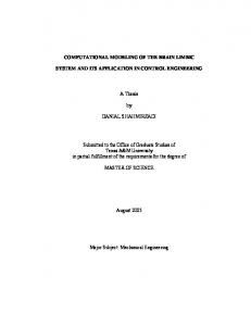
Introduction The problems of animating articulated figures with multiple legs have long been a source of difficulty in the computer animation field. Joint angle interpolation between ~key" joint positions is the most widely used method of animating jointed animals. This method fails to work, however, for cases in which the end of a limb must be constrained to move along a particular path - the interpolated joint positions of two "key" leg positions planted on the ground will not, in general, remain on the ground (fig. 1). Another difficulty is the sheer tedium of positioning "keys" for limbs containing many degrees of freedom. The animal shown in figure 2 possesses 9 degrees of freedom in each leg,g degees of freedom in the neck, and 18 degees of freedom in the "spine." An animator using a key joint system would have to manage positioning a total of 63 joints. A further problem is that a walking or running figure is more than an assemblage of moving limbs - the coordination of legs, body and feet are functionally related in a complex fashion. The motion of the body of 3 figure and the timing and placement of legs are both kinematically and dynamically eoupled.[20-36] The approach taken in the design of the PODA system is to provide the animator with a computational model which facilitates the integration and direct control of the functional dependencies between

different parts of a figure. An interactive menu-driven interface is used for both the incremental construction and behavioral control of animals possessing any number of legs composed of any number of joints. A strategy is implemented in which the figure's motion may be designed and manipulated at different levels of control. At the lowest level the animator may define and adjust the character of the movement of the legs and feet. At a higher level the animator may direct the coordination of the legs and control the overall motion dynamics and path of the body. The primary goal of our efforts is to build a framework in which the synthesis of legged figure motion may be artistically conceived and controlled at increasingly higher levels of complexity and abstraction. In this regard, our initial efforts have been focussed on developing a general model tot legged locomotion due to its importance to the execution of more complex motor skills, such as those which are required for dance and gymnastics1271. In this first section we will outline the solution taken in PODA for the control of single limbs. This will set the stage for the discussion of the legged locomotion model which utilizes the limb control methods described.

Ketj2 Position

Inlterpoltt~ed Pos~ior,

Ketj 1 PosHion

F~.t 1 The research described in this paper was supported, in part, by National Science Foundation grant DCR-8304185, and in part, by a National Science Foundation Fellowship. Permission to copy without fee all or part of this material is granted provided that the copies are not made or distributed for direct commercial advantage, the ACM copyright notice and the title of the publication and its date appear, and notice is given that copying is b~, permission of the Association for Computing Machinery. To copy otherwise, or to republish, requires a fee and/or specific permission.

© 1985 ACM 0-89791-166-0/85/007/0263 $00.75

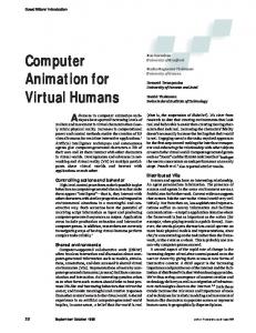
T H E C O N T R O L OF L I M B S Representing articulated limbs In order to define the functionality of all arbitrary articulated figure, PODA has adopted the kinematic notation presented by Denavit and Hartenberg {3]. This specifies a unique coordinate system for every individual degree of freedom present in the figure. These degrees of freedom, whether rotary or prismatic, will be referred to as joints and the fixed interconnecting bodies as links. The four parameters used to define the transformation between adjacent coordinate systems are the length of the link a, the twist of the link c~, the distance between links d, and the angle between links 0. The single variable associated with the transformation depends on the type of joint represented, that is 0 for rotary or d for prismatic joints (fig. 3).

263

SIGGRA

@

PH

'85

Fk~,'e 2

Given the above definitions, it can be shown I12] t h a t the transformation between adjacent coordinate frames i - I and i denoted by i-17"~ is given by the homogeneous transformation:

'-17~ =

0

The solution adopted by P O D A is to linearize the equations a b o u t the current operating point. Tile six-dimensional vector representing an incremental change in position and orientation in three space of an arbitrary link is linearly related to the vector A~" by the Jacobian m a t r i x J through the equation

0

~=

J(03~¢

(1)

where ai C O S ~i

n z = C O S @i

Pu = ai sin Oi

n u = sin ~i

Pz = dl

nz = 0

Pz =

ox = -- c o s ~ i s i n 0 1

az = s i n a i s i n O i

% = cos ~i cos ~i

a u = -- sin ~i cos ai

oz = sin a l

az = cos a l

By repeatedly applying adjacent link transformations the relationship between any two coordinate systems i and j is easily obtained using 'Tj = i'/~+t i + t 7 ~ + 2 . - - i - l T y The above equation permits any link of the figure, defined in its own coordinate frame, to be represented in any a r b i t r a r y reference or world coordinate frame. More i m p o r t a n t l y , it can be used to d e t e r m i n e the n u m b e r and characteristics of the degrees of freedom available for s i m u l a t i n g coordinated m o v e m e n t . The Jaeobian Matrix Given the above framework, one can easily see t h a t , given the s t a t e of the j o i n t angle variables, we can c o m p u t e the position of all of the links and arrive at the position of the end of the limb. This is called the f o r w a r d k i n e m a t i c s problem. The reverse situation, t h a t of c o m p u t i n g the j o i n t angles from the position of the end of the limb, is necessary if we wish to place a foot or hand in some desired p l a c e - w h a t Korein and Badler have called "goal directed motion" [32]. This is called the inverse k i n e m a t i c s problem. The legged locomotion models in P O D A rely heavily on the need for goal-directed motion: feet must be moved along trajectories, placed exactly at desired footholds and held in place as the body passes over them. The solution of the inverse kinematics problem is the source of much of the difficulty in dealing with controlling articulated figures. A general solution for arbitrary articulated chains does not exist and even those t h a t lend themselves to an analytic solution result in nonlinear equations [12]. Additional complications are incurred when r e d u n d a n t degrees of freedom are present.

264

for changes which are sufficiently small. Thus by u p d a t i n g the Jacobian each cycle time, the a d v a n t a g e s of a linear system are obtained. This allows the application of all of the techniques of solving linear equations to obtain the desired result (to be discussed in the next section). The use of Jacobians has long been a common practice in nonlinear control system theory and has been successfully applied in the field of robotics [t8,191. Due to its central nature in the a n i m a t i o n of articulated figures, an efficient i m p l e m e n t a t i o n for generating the Jacobian is essential to a viable system. While there are may different techniques available, a particularly elegant method has been formulated with the use of screw motor variables [17]. A screw motor is characterized by the variables C, the angular velocity of the screw axis, and fi, the velocity of a poiut attached to the screw axis which coincides with the origin of the world coordinate frame. In terms of these variables, the desired displacemeut of the foot may be expressed as = RC s

with the original foot displacement A:~ given by

where R is the upper 3 x 3 r o t a t i o n p a r t i t i o n of the homogeneous transformation describing the desired point whose velocity is being specified and ~ff is the position of this point given by the fourth column of its homogeneous transformation. It can be shown [16] t h a t the Jacobian is given by j=[ptxal

p2Xa2 a I

U2

p. x a . 1

... ..

•

an

(3}

J

where a4 and Pl are the third and fourth columns, respectively, of the homogeneous transformation m a t r i x ° T , _ t . The first c o l u m n of the Jacobian is given by pl = [000t T

at =[0011T

,

SAN FRANCISCO JULY 22-26

Volume 19, Number 3, 1985

Fujure $

the null space of the transformation. The physical interpretation of the homogeneous solution is illustrated in figure 4. Thus by different choices for the vector Z, various desirable properties described in ~-space can be achieved under tile constraint intposed by exact achievement of the specified A£. One particularly useful property is to keep joints asclose as possible to some particular angles chosen by the animator. This is done [81 by specifying the vector iin equation (6) to be

j o i n t I~ I

z

i-cx~ ~

'

~=XTH with H = ~c~;(Oi i=1

,ink

x~.~ Link P a r a m e t e r s Associated With Link i

This formulation of the Jacobian allows a m i n i m a l a m o u n t of e x t r a c o m p u t a t i o n since the majority of the work has already been done in generating the homogeneous transformations required to display the object. This is in contrast with other techniques which do not express the Jacobian in the world coordinate frame [37 I. Inverting the Jacobian Given a linear system by virtue of the Jacobiau, we uow need to invert the relationship represented by equation (1} in order to determine the required AO to achieve a desired ~:~. Since we are dealing with arbitrary articulated figures, the Jacobiau is in general not square and therefore its inverse is not.defined. To obtain a useful solution regardless of the rank of J, the pseudoiuverse is applied. The pseudoinverse will be denoted by J + and is the unique [[3] m a t r i x which satisfies the four properties:

- e,.,) ~"

where Oi is the i t h joint angle, O,:~ is the center angle of the i t h j o i n t angle, and ~i is a center angle gain value between zero and one. The equation may also be generalized for H equal to any smooth function one wishes to minimize. The center angles define she desired j o i n t angle positions and their associated gains define their relative importance of satisfaction. From the a n i m a t o r s point of view, the gains may be t h o u g h t of ~ "springs" which define the stiffness of the j o i n t a b o u t some desired center position. PODA provides interactive specification of center angles and gains as a means of controlling r e d u n d a n t degrees of freedom in the legs. The implementation of this formulation can be included in the gaussian elimination procedure for c o m p u t i n g the pseudoinverse if it is properly decomposed 171.

Figure 4

dd+J=J J+ J J+ = J+ ( g + J)T = j + j (j j+)T = j j+

(4)

The advantages of using the pseudoinverse lie in that it returns the least squares m i n i m u m norm solution to equation (1). Thus it provides useful results in both the under and over d e t e r m i n e d cases. Other generalized inverses m a y also be applied [1,2]. An excellent overview concerning the pseudoinverse control of r e d u n d a n t m a n i p u l a t o r s as well as a geometric interpretation of the pseudoinverse using singular value decomposition is presented in [7I. A number of different methods for calculating pseudoinverses have been discussed in the literature [6,14]. A discussion of the some of the numerical considerations involved in computing the pseudoinverse is presented by Noble [11]. The simplest expressions for a pseudoinverse appear for matrices known to be of full rank. For an rn × n matrix A of rank r, the expression for the pseudoinverse is given by

A+= f(AT A)-IA T A T (A A r )

ifm>n=rand if r = rn < n

The use of Gaussian e l i m i n a t i o n w i t h pivoting removes the need for an explicit inverse calculation and results in a stable and efficient technique %r computing the pseudoinverses under these conditions. For matrices of unknown rank a recursive procedure for c o m p u t i n g the pseudolnverse presented by Greville [4] may be used, the details of which are beyond the scope of this paper. Controlling Redundant Limbs in PODA While the above section illustrates how the pseudoinverse can be used to obtain a useful solution to equation (1), for cases where redund a n t degrees of freedom exist, it is only one of an infinite n u m b e r of solutions. The m a n n e r in which the a n i m a t o r is given the flexibility to determine which of the available solutions is most desirable is through a projection operator. It can be shown t h a t shown 15] that the general solution of equation (1) is given by

where I is an n × n u n i t y m a t r i x and z is an a r b i t r a r y vector in A 0 spac6. Thus the homogeneous portion of this solution is described by a projection operator ( I - J + J ) t h a t marts the arbitrary vector ~ into

Homogeneous solu'tion to ~he de¢obien equation is 'the set of joint velooities ~,hich cause no end effector motion. MODELING THE KINEMATICS OF LEGGED LOCOMOTION The task of a kinematic model for legged locomotion is to coordinate the motion of the legs,feet and body in terms of their respective positions and velocities (Newtonian mechanical properties such as force and mass are not considered). The kinematic model must enable the animator to design the timing relationships between the legs and the character of the steps taken by each leg in accordance with the design of the body's trajectory, orientation and speed. Ideally, it should be easily adaptable to any extensions made in the dynamics domain. G a i t ] D e s i g n in P O D A T h e m o d e l of locomotiou i m p l e m e n t e d in P O D A utilizes a n u m b e r of p a r a m e t e r s which are convenient for describing the gait of a figurethe terms and relations are derived from robotics research on walking machines [22-26]. A gait pattern describes the sequence of lifting and placing of the feet,. The p a t t e r n repeats itself as the figure moves: each repetition of the sequence is called the gait cycle. The time (or n u m b e r of frames) t a k e n to complete a single gait cycle is the period P of the cycle. The relative phase of leg i, Ri , describes the fraction of the gait cycle period which transpires before leg i is lifted. The relative phases of the legs m a y be used to classify the well known gaits of q u a d r u p e d a l animals (fig. 5). During each gait cycle period any given leg will spend a percentage of t h a t time on the g r o u n d - t h i s fraction is called the duty factor of le 9 i. For example, the d u t y factor m a y be used to distinguish between the w a l k i n g and running gaits of bipeds. W a l k i n g requires t h a t the d u t y factor of the each of the legs exceed 0.5 since, by definition,the feet must be on the ground simultaneously for a percentage of the gait cycle period. Lower d u t y factors (less t h a n 0.5) result in balhstic motion identified with running, wherein the entire body leaves the ground for some duration.

265

¢°~ S I G G R A P H '85

amble

trot

paca

center

0

0

0

0

0.5

0.5

0.5

legState = (legState 0 + t) mad P

(9)

where

0.3

legState,) = ( R ~ ) (P) ff

0

0

0.5

0.7

0

0.1

0

0

0

0

foot liftoff occurs when the leg state is equal to the support duration (fig.7).

0 . 7 5 0.25 0.~ 0

0.5

0.1

0.6

0

0.6

05

0.50.S

0

troverse rotorql Imoml gallop eollop

An animator using P O D A may design gaits for figures having any number of legs by instantiatingthe parameters given above. The mode[ makes sure that all the variables axe updated according to functional dependencies, thereby freeingthe animator to experiment with the variables of interest such as relative phase without worrying about the integrity of the other related variables.

0

proak Figure5

We will call the time a leg spends on the ground its support duratmn. The time spent in the air is the leg's transfer duration. The stroke is defined as the distance traveled by the body during a leg's support duration. If we acknowledge that the foot must traverse the stroke during the transfer phase in order to "keep up" with the body, the stroke may alternatively be regarded as the length of the step taken by the leg over the ground (fig. 6a). The body may move over the ground plane in PODA, so the stroke in this context becomes the diameter of a circle in that plane (fig. 6b).

6a

"~i~

T r e n s f e r ~

Leg S u p p o r t and Transfer Trajectories

- stroke, - - - - - > z

Figure Gb

I J

Leg Coordination The following relationship holds between the legs and the body: stroke s u p p o r t D u r a t i o n - bodySpeed

(7)

The above equation solves for the time (or number of frames) that each leg must spend on the ground. By definition we also have d u t y F a c t o r - snpportDuration P The amount of time which a leg spends in the air depends on both the leg speed and the arclength of the transfer phase trajectory. That is: transferDuration = arcLength(transferTrajectory) legSpeed During the gait cycle period P, a single leg will move through one cycle of support and transfer, hence we have: P = supportDuration + transferDuration

(8)

for any leg k. In fact, one may imagine the period as a duration subdivided into support and transfer durations {fig. 7). The le e state at time t may be determined as

266

Foot Placement

Fo.t~~e~ :d~~ DS~rP~tnePt~. Liftoff F'kWe7

..... ~'~- ~ Figure

the leg state is less than the support duration then the leg is in

its support phase, otherwise the leg is in its transfer phase. Moreover, the time of foot placement occurs when the leg state equals zero and the

Aside from the problem of coordinating the timing of the legs, one must design the motion of the step taken during the transfer phase and insure that the feet will remain planted on the ground during the support phase. A step is specified in PODA by the desired trajectory of the feet and the center angles and gains on the joints (which may change dynamically). The curve which defines the foot trajectory is defined by a Catmull-Rom (interpolating) spline. Because the desired shape o[ the curve depends oR the geometry of the leg, the control points of the sptine are set by moviug the foot of the leg. The animator may conceptualize the design of the step as tile specification of "key leg positions," in the spirit of a key-framing system. In PODA, a key position records the position of the foot (as a control point in the spline} and the center angles and gains that are associated with that position. The animator manipulates the foot into each position using PODA's inverse kinematic procedm'es, and then , once the foot is in place, the joint aneles may be adjusted using the center angle and gain parameters. This approach is distinguished from key-framing or joint angle interpolation systems in that the goal of achieving the desired foot position in Cartesian space is primary-the foot will travel precisely along the smooth CatmulI-Rom spline from foothold to foothold. By contrast, ff we interpolate the the leg positions in joint space, there is no general means of either moving the foot along a curve or placing the foot at a particular place on the ground. The problem of keeping the legs on the ground as the body translates and rotates is simplified due to PODA's inverse kinematic capability. The problem reduces to solving for the position of the foot in the leg's moving coordinate system so that it is identical to the placement of the foot in the previous frame's world coordinate system (thereby keeping the foot stationary in the world). We we solve for this position using: (

\

w rl prevFrameFoo~_ t = wor, THip~_, (HipFoo-HiI'prevFrameFoott = H i P T w o r l d ,

(

\

(10) /

')

W°rldprevFrameFoo~_~

SAN FRANCISCO JULY 22-26

Volume 19, Number 3, 1985

Directional Control of the Body

If the animator is to have supervisory control over the legged figure, a means for directing the body's full translational and rotational degree's of freedom must be available. Given that all the legs are on the ground, the problem may be solved using equation {10). The fundamental problem is to calculate footholds and plan the foot transfer trajectories between them so as to adapt to the desired body motion. Foothold and Transfer Trsjeetory Planning An important concept of foothold planning is the notion of a reference leq position[221. This is the desired position of the leg in midstance or half way though the leg's support duration (fig. I0). The posture of an animal when all of its legs axe in their reference positions may be regarded as the "standing" position of the animal (fig. ll). The other key ingredient for the foothold calculation is the ability to predict the body's future positions. In PODA, the body's trajectory may be computed as a function of the desired body trajectory over the ground plane [a cubic spline designed by the animator) and dynamic constraints due the timing and force limitations of legs (to be discussed) before the precise footholds are chosen. Since the body's position is known in advance, it is possible to plan ahead in order step toward the next stable position

The primary design concerns of the robotics algorithms are to maintain dynamic stability of the walking vehicle, to avoid leg intersections, to optimize the load balancing and energy consumption, and to insure that the feet never stray beyond their kinematic limits. Because the algorithms must actually work for real walking machines (rather than simulated figures), their scope is conservative. Restrictions are placed on the types of gait patterns and relative phase relationships between the legs, thereby drastically limiting the repertoire of behaviors. The design philosophy of PODA is tu give the animator absolute control over the entire set of of available gaits in order to exploit the coupling between rhythm and dynamics (to be discussed) since these matters are of extreme importance in artistic design. Moreover, since PODA's current implementation on the Ridge 32C minicomputer prorides for realtime computation of a figure possessing four 9-degree of freedom legs at 2 frames per second, leg interference and unnatural leg stretching may be detected immediately, leaving the range of many reasonable solutions to these problems up to the artist rather than hard-wiring a single solution into the motion model.

MODELING

Fool Pllceemen't ........

~.-, .

.

.

q i I

)

.

'~, X X\\ \ \

Foot

reference leg positi0n

,'~

Lift Off -1 I

0,...2

l

)

t~

I / II I

I ! i . _ jI

At the beginning of the leg transfer phase of leg z, say at frame t, we must compute the reference leg positiou in world space at frame ft as follows: W"rtATHipq = W"~ldTB,,,ivtl B'"WTHi p

w'"t'trefLegPosl, = w""t'tTHil, t, ( u i v r e F L e ~ s)

(IL)

where fl = t + transferDuration + 0.5(supportDuration) This foothold will insure that that leg z comes to its "mid-stance" position half way through its support phase. We umst still determine the position of the foot in the body's coordinate system at the time the foot is placed down. This knowledge is required in order to facilitate moving the foot horizontally with respect to the body during the transfer. This may be accomplished by: n"aYrefLegPosf: = B"'tYTw,,rldf~

(

W"rl~l~f

THE DYNAMICS

OF L E G G E D L O C O M O T I O N The simulation of the dynamics of motion control in legged animals is an extremely complex modeling problem. Models for single limbs (industrial robots) which compute the relationships between the torques applied at the joints,the masses and moments of inertia of each of the links, and the position of the joints and their associated time derivatives, are well understood [381. Work has also been published in the biomechanics field on the the relationship between muscular forces and motion parameters of simplified "ideal" models of animals[33,341. Although these models may produce interesting animation, their appropriateness for artistic design and control must be considered as well as their (usually substantial) computational costs.

Mid-5~anoe =

t

)

where

f2 = t + transferDuration The generic transfer trajectory designed by the animator may then be adapted to move between the current foot position and the calculated foothold so that the height in the world and proportional distance moved next to the body are preserved. Robotics research on walking vehicles has provided a rich source of computational models for the solution of body motion planning and leg coordination[22-261. However, their design criteria is somewhat different the requirements of animation.

S i m u l a t i o n vs. A n i m a t i o n In contrast to industrial robots and biomechanical simulations, animation does not necessarily require the computation of actual forces. The application of dynamics to animation is simplified by the fact that we are interested only in what can be seen. The essential concern is to make the motion look as if forces were being applied. In other words, we are primarily interested in solving for the acceleration in dynamics models - the computation of parameters such as forces, torques and moments of inertia is only relevant if it can help us easily manipulate accelerations to produce coherent dynamic realism. The necessity for modeling dynamics in PODA was apparent as soon as the kinematic model was completed. In a purely kinematic model the motion of the body is quickly seen to be independent from the coordination of the legs, and it appears as though the body is suspended from strings, pulling its legs behind it. The development of dynamics for PODA is an ongoing research project. The initial goal was to see whether very simple dynamic models of legged locomotion could be developed which were both amenable to artistic control and as fully general as the kinematic nmdel (applicable to any figure constructed by the animator}. At the time of this writing, PODA is capable of modeling the translational acceleration of the center of mass of body in the vertical direction and ground plane, and the rotational acceleration of the body that is required to insure that it is facing in the direction of movement (if turning is desired}. At all stages, the body's motion is constrained and propelled by the simulated forces applied by the legs. D e c o m p o s i t i o n o f D y n a m i c C o n t r o l in P O D A The simple model used in PODA was inspired by Raibert's work on legged hopping machines. He and his coworkers have built a onelegged hopping machine which is able to balance and move in three dimensions. His control algorithms are based on a decomposition into hopping height, forward velocity, and attitude control[31,28]. The model used in PODA decomposes the dynamic coupling between the legs and the body along two lines: decomposition by leg and decomposition by body direction. Vertical C o n t r o l Dynamics in the vertical direction must take into account the effects of gravity and the gait cycle period of each leg. Since PODA's decomposition scheme is based on decomposition by leg, it will be helpful to consider a one-legged figure.

267

~o5 S I G G R A P H '85

WT¢, Moving in a wave gait, the legs near the rear advance toward their next footholds.

A 14 legged insect shown in its standing position. Figure 1 1 The current model makes the simplifying assumption that the upward force applied by the leg on the body is constant during its support phase. The animator supplies PODA with both the value of this force, the mass of the body, and the downward acceleration due to gravity• Net upward acceleration of the center of mass is then given by: =

ma ssb,,dy

g

for leg i

(12}

The gait cycle period may be subdivided into three dynamic stages of the leg's motion: pushing the body up,free falling,and then restoring the body to its original position (as long as the application of upward leg forces are symmetrical about the mid-stance position, the body will stabilize to zero velocity at that position}. We will call these the push duration, fall duration, and restore duration respectively (fig. 12). The leg support duration is a function of the body speed in the horizontal plane and the stroke (equation 7). Since the leg's traversal of the transfer trajectory must coincide with the body's ballistic motion, we have: t ..... ferDurati . . . .

(?)

(support Duration)

However, a legged figure's acceleration toward a desired direction and speed must be coherent with its leg support duration pattern and it must also simulate the effects of momentum in a given direction in order to give the body a sense of weight. In PODA, the body's ability to turn and speed up is consistent with the number of feet on the ground and the maginitude of the maximum achievable force [[Fm~x~ll assigned by the animator to each supporting leg. The maximum achievable acceleration of the body is governed by the sum of their forces:

i=

ntassh,),ly

where n is the number of feet on the ground.

(13)

The vertical position of figures with multiple legs is determined in PODA by the superposition of the ballistic motion of the body due of each of its legs considered independently. This extremely simple model produces relnarkably realistic motion for both walking and running in multiple leg figures: if the magnitude of vertical acceleration is low and the phase relationships of the legs are in opposition, the upward accelerations will cancet, resulting in asmooth walkingoscillation. High accelerations resulting from strong single leg forces (e.g. running in a trot) or the sum of forces of many legs pushing from the ground together (e:g. hopping) propel the body into the air. The trajectory taken by the body due to the summation of vertical leg accelerations and downward gravitational accelerations taken from each of the legs is automatically synchronized with rhythm of the phase relationships in the legs. For example, convincing cantors, trots, and bounding motion may be animated simply by altering the figure's gait. Another advantage to PODA's leg decomposition of vertical dynamics is that changes in the figure's motion parameters which evolve over gait cycle periods, such as body speed or upward leg force may be easily accommodated by adjusting the related dynamic parameters for each leg's contribution independently at the beginning of its upward pushing phase. The stability of each leg's contribution guarantees the vertical stability of the body as a whole. A gait shifting algorithm has been developed by one of the authors which exploits the ability for legs to undergo phase shifts by varying the distribution of vertical pushing forces among them.

Ou/ ,.on// / /

.. ~ ..~ /,~ ~ Cl I L

]Transfer

Horizontal Control The desired horizontal path taken lhy the figure is specified in PODA by the animator with a cubic spline (Catmull-Rom or B-spline). Given the desired body speed along different parts of the curve, PODA may calculate the desired positions and velocities along it using a numerical arclength calculation.

;2, - X ~uppport Duration

r-.-,

tOuratio,

Period

Push

tifloff

~'-'~-'"'Dur

at ion

Figure t 2

At each frame PODA computes the next desired velocity along the desired bouy path. Then PODA determines the desired acceleration at a given frame through velocity error feedback, that is, by subtracting the desired velocity from the current velocity at that frame. The horizontal acceleration of the body at frame t is tllen computed as: ..............

(15)

where

li~=ll

268

i

at:

= min(ll~:~

I, ;i~, I =

............ II,II~=.......II)

h'sir,',l - Vel

An additional backward acceleration during the restore duration and forward acceleration during the push duration is necessary in order to sinmlate the effects foot position with respect to the body at foot

placement and foot liftoff [28]

SAN FRANCISCO JULY22-26

Volume 19, Number 3,1985

Rotational Control The foothold and leg transfer calculations described adapt to allow for full rotational control of the body. At the time of this writing, however, only the dynamics of accelerati.ons about the yaw axis have been implemented (the pitch axis rotation apparent in figurei 2 is due to the separation of the application of vertical acceleration between the front and rear sections of the body). Y a w axis accelerations are necessary if we wish the body to realistically turn so that it is facing in the direction of movement. The simple frame to frame strategy applied for horizontal control is not sul~cient for coordinated turning, especially for running gaits wherein the legs are off the ground. In such cases one must know where the body is going in order to effectively anticipate the rotational accelerations required to keep the body properly oriented before its feet leave the ground. The solution adopted by P O D A for rotational control takes advantage of its ability to know the translatioual coordinates of the body in advance. The order of calculation for body dynamics plays an important role in this matter (fig. 13). The direction of body motion m a y be derived from the sequence of actual velocities taken by the body.

Animatorinputs ] DesiredBodyPath endBodySpeed $

vCOmputeDesired I elocltg along Path ] D

4,

J ComputeHorizontaland ] Vertical BodyDynamics ] I ComputeAngularBody I Dynamics

Figure 1$

BodyPosition andOrientation

REFERENCES [1[ Ben-lsrael, Adi and Thomas N. E. Greville, "Generalized Inverses: Theory and Applications," Wiley-lnterscience, New York, 1974. [21 Bouillon, T. L. and P. L. Odell, =Generalized Inverse Matrices," Wiley-lnterscience, New York, 1971. [3] Denavit, J. and R. S. Hartenberg, =A Kinematic Notation for Lower-Pair Mechanisms Based on Matrices," ASME Journal o[ Applied Mechanics, Vol. 23, pp. 215-221, June, 1955. I4] Greville, T. N. E., "Some Applications of the Pseudoinverse of a Matrix," SlAM Review, Vol. 2, No. 1, January, 1960. [5] Greville, T. N. E., "The Pseudoinverse of a Rectangular or Singular Matrix and its Applications to the Solutions of Systems of Linear Equations, n SIAM Review, Vol. 1, No. 1, January, 1959. I6} Hanson, R. J. and C. L. Lawson, =Extensions and Applications of the Householder Algorithm for Solving Linear Least Squares Problems," Mathematics of Computation, Vol. 23, pp. 787-812, 1969. [71 Klein, C. A. and Hnang, C. H., =Review of Pseudoinverse Control for Use with Kinematieally Redundant Manipulators," IEEE Transactions on Systems, Man, and Cybernetics, Vol. SMC-13, No- 2, pp. 245-250,March/April, 1983. [8] Liegeois, A., "Automatic Supervisory Control of the Configuration and Behavior of Mu|tibody Mechanisms," IEEE Transactions on Systems, Man and Cybernetics, Vol. SMC-7, No. 12, December, 1977. [9] Maciejewski, A. A., and Klein, C. A., "Obstacle Avoidance for Kinematically Redundant Manipulators in Dynamically Varying Environments," to appear in International Journal of R o b o t i ~ Research. [1OJ M~iejewski, A. A., and Klein, C. A., "SAM - Animation Software for Simulating Articulated Motion," submitted to IEEE Computer

Graphics and Applications. Once the desired body orientations are known, PODA is able to exploit the leg decomposition strategy employed for vertical control. Each leg applies a positive acceleration during its pushing phase and a negative restoring acceleration during its restoring phase in order to bring the body exactly to the desired angle computed at its mid-stance reference leg position. If we solve Newton's equations of motion with the constraint that we wish the final mid-stance rotational velocity to be zero, we have: ( a | n i d S t r u l c e + P -- O'midStaltce )

5 : (pnshDuration)(pushDuration + failDuration) where ¢7 is angle about the yaw axis. Conclusion The described formulations have proven to be successful models fol the synthesis of legged locomotion. However, many interesting problems remain to be solved. We will refine the legged locomotion model in PODA as more is learned from each simpler model. The addition of rotational dynamics for body pitch and, more generally, the modeb ing of body dynamics due to the motion of non-supporting limbs are obvious choices for extension. Other problems of interest include the development of control techniques for maintaining postural balance, the inclusion of obstacle avoidance and collision detection, and a means of designing motor skills above and beyond the requirements of walking and running. Acknowledgements The authors wish to thank John Runner and Susan Amkraut for the preparation of this document, and Charles Csuri and Thomas Liuehun for their maintenance of the stimulating environment at C G R G .

[II] Noble, B., "Methods for Computing the Moore-Penrose Generalized Inverses, and Related Matters," pp. 245-301, in Generalized Inverses and Applications, ed. by M. A. Nashed, Academic Press, New York, 1975.

[12] Paul, R., Robot Manipulators, MIT Press, Cambridge, Mass., 1981. [13] Penrose, R., =On Best Approximate Solutions of Linear Matrix ,.,quations," Proc. Cambridge Philos. Soc., Vol. 52, pp. 17-19, 1956. [14] Peters, G. and J. H. Wilkinson, =The Least Squares Problem and Pseudo-Inverses, ~ The Computer Journal, Vol. 13, No. 3, August, 1970. [15] Ribble, E. A:, =Synthesis of Human Skeletal Motion and the Design of a Special-Purpose Processor for Real-Time Animation of Human and Animal Figure Motion," Master's Thesis, The Ohio State University, June, 1982. [16[ Waldron, K. J., "Geometrically Based Manipulator Rate Control Algorithms", Seventh Applied Mechanics Conference, Kansas City, December, 1981. ]17] Waldron, K. J., =The Use of Motors in Spatial Kinematics," Proceedings of the IFToMM Conference on Linkages and Computer Design Methods, Bucharest, June, 1973, Vol. B., pp. 535-545. [181 Whitney, D. E.~ "Resolved Motion Rate Control of Manipulators and Human Prostheses," IEEE Transactions on Man-Machine systems, Vol. MMS-I0, No. 2, pp. 47-53, June, 1969. [19] Whitney, D. E., "The Mathematics of Coordinated Control of Prostheses and Manipulators, ~ Journal of Dynamic Systems, Measurement, and Control, Transactions ASME, Vol. 94, Series G, pp. 303-309, December, 1972, pp. 49-58.

269

Q

[201 Alexander, R., "The Gaits of Bipedal and Quadrupedal Animals," The International Journal of Robotics Research, Vol. 3. No. 2, Summer 1984. [21] McOhee, R.B., and Iswandhi, G.I., "Adaptive Locomotion of a Multilegged Robot over Rough Terrain ~, IEEE Transactions on Systems, Man, and Cybernetics, Vol. SMC-9, No. 4, April, 1979, pp. 176-182. [22] Orin, D.E., "Supervisory Control of a Multilegged Robot", International Journal of Robotics Research, Vol. 1. No. 1, Spring, 1982, pp. 79-91. 123] Klein, C.A., Olson, K.W., and Pugh, D.R., ~Use of Force and Attitude Sensors for Locomotion of a Legged Vehicle over Irregular Terrain, ~ International Journal of Robotics, Vol. 2, No. 2, Summer, 1983, pp. 3-17. [24] Ozguner, F., Tsai, L.J., and McGhee, R.B., "Rough Terrain Locomotion by a Hexapod Robot Using a Binocular Ranging System," Proceedings of First International Symposium of Robotics Research, Bretton Woods, N.H., August 28, 1983. [25[ Lee, Wha-Joon, "A Computer Simulation Study of Omnidirectional Supervisory Control for Rough-Terrain Locomotion by a Multilegged Robot Vehicle," Ph.D. Dissertation, The Ohio State University, Columbus, Ohio, March, 1984. [26] Yeh, S. "Locomotion of a Three-Legged Robot Over Structural Beams," Masters Thesis, The Ohio State University, Columbus, Ohio, March, 1984. [27] Zeltzer, D.L., "Representation and Control of Three Dimensional Computer-Animated Figures," Ph.D Dissertation, The Ohio State University, Columbus, Ohio, March, 1984. [28] Murphy, K.N., and Raibert, M.H., "Trotting and Bounding in a Planar Two-Legged Model," Fifth CISM-IFTOMM Symposium on Theory and Practice of Robots and Manipulators, June 26-29, 1984, Udine, Italy. [29] Miura, I-I. and Shimoyama, I. "Dynamic Walk of a Biped," The International Journal of Robotics Research, Vol. 3, No. 2., Summer 1984, pp 60-74. {301 Pearson, K.G., and Franklin, R., "Characteristics of LegMovements and Patterns of Coordination in Locusts Walking on Rough Terrain," The International Journal of Robotics Research, Vol. 3, No. 2., Summer 1984, pp 101-107. [31] Raibert, M.H., Brown, H.B.Jr, and Chepponis, M., "Experiments in Balance with a 3D One-Legged hopping Machine, ~ The International Journal of Robotics Research, Vol. 3, No. 2., Summer 1984, pp 75-82. [32]. Korein, J.U., and Badler, N.I., "Techniques for Generating the Goal-Directed Motion of Articulated Structures," IEEE Computer Graphics and Applications, November 1982, pp. 71-81. [33] Hemami, H. and Zheng, Y., "Dynamics and Control of Motion on the Ground and in the Air with Application to Biped Robots," Journal of Robotic Systems, Vol 1. No. 1, 1984, pp. 101-116. [341 Hemami, H. and Chen, B. "Stability Analysis and Input Design of a Two-Link Planar Biped, The International Journal of Robotics Research, Vo[. 3, No. 2., Summer 1984, pp. 93-100. [35] McMahon, T.A., "Mechanics of Locomotion," The International Journal of Robotics Research, Vol. 3, No. 2., Summer 1984, pp 4-18. [36] Luudin~ R.V. "Motion Simulations" Nicograph Proceedings 1984, pp. 2-10. [37] Orin, D. E., and Schrader, W. W , "Efficient Jacobian Determination for Robot Manipulators~" Sixth IFToMM Congress, New Dehli, India~ December 15-20, 1983.

270

S I G G R A P H '85

[381 Orin, D.E., McGhee, R.B., Vukobratovic, M.,and Hartoch, G., "Kinematic and Kinetic Analysis of Open-Chain Linkages Utilizing Newton-Euler Methods," MathematicM Bioscienees,Vol. 43, lp. 107-130, 1979.