computational modelling of single crystals 1 ... - Semantic Scholar

Modeling and Simulation in Material Sciences and Engineering, 1:(3),pp. 225–263.

COMPUTATIONAL MODELLING OF SINGLE CRYSTALS ˜ and Michael Ortiz Alberto M. Cuitino Division of Engineering Brown University Providence, RI 02912, USA

Abstract The physical basis of computationally tractable models of crystalline plasticity is reviewed. A statistical mechanical model of dislocation motion through forest dislocations is formulated. Following Franciosi and co-workers, the strength of the short-range obstacles introduced by the forest dislocations is allowed to depend of the mode of interaction. The kinetic equations governing dislocation motion are solved in closed form for monotonic loading, with transients in the density of forest dislocations accounted for. This solution, coupled with suitable equations of evolution for the dislocation densities, provides a complete description of the hardening of crystals under monotonic loading. Detailed comparisons with experiment demonstrate the predictive capabilities of the theory. An adaptive finite element formulation for the analysis of ductile single crystals is also developed. Calculations of the near-tip fields in Cu single crystals illustrate the versatility of the method.

1 INTRODUCTION Ductile single crystals are of considerable interest in single phase form, e. g., as structural materials in propeller and turbine blades, or as basic building blocks of numerous material systems, such as polycrystalline metals and igneous rocks. Many deformation processes of interest take place at the single crystal level. Notable examples include the development of deformation textures in polycrystalline metals, shear band formation within grains, crack nucleation and growth at grain boundaries, transgranular cracking, and others. Recent advances in computer hardware and software have made ever more detailed simulations of ductile single crystals and polycrystals possible. Impetus for this type of simulations is provided by a desire to root models of the behavior of solids on a sound micromechanical basis. There is, therefore, a need for computationally tractable models which emanate directly from a clear micromechanical picture, as well as for robust and versatile computational techniques for incorporating the models into numerical simulations. Our first aim here is to review dislocation theories which, in combination, point to a plausible form of the hardening relations for single crystals. The theories considered concern: i) the motion of a dislocation line through forest dislocations; ii) the short-range interactions between pairs of dislocations and the strength of the resulting intersections viewed as point obstacles, and iii) the kinetics of dislocation multiplication. It bears emphasis that, in the simple physical picture contemplated here, hardening is assumed to be primarily the effect of forest dislocations. Simple though it may be, a satisfactory aspect of this theory is that it is amenable to a rather rigorous analytical treatment within the framework of non-equilibrium statistical mechanics. Indeed, we show that, for monotonic loading, the kinetic equation governing the percolation-like motion of a dislocation line through a random array of point obstacles can be solved in closed form. Our solution includes the case in which the density of point obstacles is a function of time. Following Franciosi and co-workers (Franciosi et al., 1980; Franciosi and Zaoui, 1982; Franciosi, 1983, 1985a, 1985b, 1988), the 1

Cuitiño & Ortiz

Computational Modelling of Single Crystals

2

strength of the short-range obstacles introduced by forest dislocations is taken to be a function of the mode of interaction, e. g., of whether the intersecting dislocations react to form junctions. Our analytical solution, in conjunction with Franciosi’s relations, completely determines the hardening relations of the crystal in terms of the density of dislocations in all slip systems. To obtain a closed set of constitutive relations, we draw on the work of Gillis and Gilman (1965) and Essmann and Rapp (1973) to formulate the requisite equations of evolution for the dislocation densities as a function of slip activity. Interestingly, the dislocation-based model reconciles some apparent differences between the recent work of Bassani and Wu (Wu et al., 1989; Bassani and Wu, 1989; Bassani, 1990), who have proposed a model in which the hardening matrix is diagonally dominant, and the more conventional approach of Pierce et al. (1983), who model latent-hardening effects by means of a hardening matrix in which the off-diagonal terms are dominant. These two models arise from seemingly diverging interpretations of the experimental record. The dislocation model developed here suggests that these views are, in fact, complementary. Thus, for each slip system, two characteristic resolved shear stresses can be identified: the elastic limit, or yield stress; and a characteristic stress roughly coincident with the value of flow stress obtained by back-extrapolation of the stress-strain curve, a procedure which is commonly adopted for the interpretation of latent hardening experiments (Kocks, 1970; Ramaswami et al., 1965; Kocks and Brown, 1966; Franciosi et al., 1980; Bassani, 1990). While increments of the former characteristic stress are related to slip increments by a diagonal hardening matrix, as in Bassani and Wu’s theory (Bassani and Wu, 1989), increments in the latter are governed by an off-diagonally dominant hardening matrix, as in the formulation of Pierce et al. (1983). Next we review some selected computational methods for the analysis of ductile single crystals. Our discussion emphasizes implicit integration and adaptive meshing techniques. A different and complementary perspective can be found in the earlier review article of Needleman et al. (1985). More specifically, we consider state updates defined a` la backward-Euler, and enforce global equilibrium and compatibility exactly at the end of each time step. It bears emphasis that the finite deformation aspects of the formulation, such as the finite rotations undergone by the lattice, are also treated exactly. We show that the state update can be reduced to a system of nonlinear equations for the incremental slip strains. This system can be efficiently solved by means of a local Newton-Raphson iteration for which the Jacobian matrix can be written down explicitly. We also give an iterative procedure for identifying the active slip systems which reduces to the conventional elastic-predictor/plastic-corrector formulation of implicit updates for singlesurface plasticity. An aspect of crystal plasticity models which is particularly attractive from the standpoint of implicit integration is that the consistent tangent moduli required to formulate a global Newton-Raphson solution procedure can be written down explicitly with some generality. This speeds up the computations by ensuring asymptotically quadratic convergence of the equilibrium iterations. Because of the crystallographic nature of slip in single crystals, plastic flow is often confined to narrow regions across which displacements and stresses vary rapidly. In cases where the geometry of the slip patterns is not known a priori, adaptive meshing techniques furnish an effective means of resolving the fine structure of the solution. Despite its obvious appeal, adaptive refinement has not been widely used in single crystal calculations. General meshing techniques and state transfer operators which are applicable to finitely deforming plastic solids have been developed by Ortiz and Quigley (1991). Here we adapt these techniques to applications concerned with cracks in single crystals. An adaptation criterion based on the equidistribution of plastic work has been found effective for tracking and resolving the intricate slip patterns which arise in those applications. The paper is organized as follows. Following some background on the general form of the constitutive relations for ductile crystals covered in Section 2, hardening relations are discussed in Sections 3 to 5, with special emphasis on dislocation models. Numerical matters related to constitutive updates and their integration into implicit solution procedures are taken up in Section 6. In Section 7, detailed comparisons with experiment are presented which demonstrate the ability of the theory to capture key features of the


Cuitiño & Ortiz


3

experimental record such as: latent hardening variations between secondary systems; variations of the onset and extent of the stages I and II of hardening with the orientation of the loading axis; patterns of slip activity; the evolution of dislocation densities, and others. As an example of application, in Sections 8 and 9 we present calculations of the near-tip fields of a crack in a copper single crystal. The calculations are based on the dislocation model developed in the preceding sections. The numerical results are compared to the small-strain analytical solutions of Rice (1987) and Saaedvafa and Rice (1989) and to the previous calculations of Mohan et al. (1992a,1992b) for Al-Cu and Fe-Si alloys. The structure of the solution is seen to depend critically on the details of the hardening law and the assumed kinematics, which illustrates the need for physically based constitutive relations finely tuned to specific classes of crystals.

2 GENERAL CONSTITUTIVE FRAMEWORK 2.1 Incremental field equations Consider a solid initially occupying a reference configuration B0 , and a process of incremental loading whereby the deformation mapping over B0 changes from n , at time tn , to n+1 n , at time tn+1 tn 4t. We enforce equilibrium at time tn+1 weakly by recourse to the virtual work principle

= +

=

Z

B0

P

Z

Pn+1 : r0 dV0

B0

fn+1 dV0

Z

@B0

+u

tn+1 dS0 = 0 f

(1)

t

where n+1 denotes the first Piola-Kirchhoff stress field at time tn+1 , n+1 and n+1 are the corresponding body forces and boundary tractions, respectively, is an admissible virtual displacement field, and r0 denotes the material gradient. Assume for now that we have determined a rule to update the stress field of the general form n+1 n+1 state at tn ; 4t

P

= P^ (F ;

where the deformation gradients

)

Fn+1 = r0n+1

are assumed given. Inserting (3) and (2) into (1) one obtains

Z

B0

(2)

P^ (r0 n+1; state at tn; 4t) : r0 dV0

Z

B0

fn+1 dV0

(3) Z @B0

tn+1 dS0 = 0

(4)

which defines a set of nonlinear equations which can be solved for the updated deformation mapping n+1 .

2.2 General constitutive framework The total deformation of a crystal is the result of two main mechanisms: dislocation motion within the active slip systems and lattice distortion. Following Lee (1969), this points to a multiplicative decomposition

F = FeFp (5) of the deformation gradient F into a plastic part Fp , defined as the cummulative effect of dislocation motion, and an elastic part Fe , which describes the distortion of the lattice. Following Teodosiu (1970) and others (Asaro and Rice 1977, Havner 1973, Hill and Rice 1972, Mandel 1972, Rice 1971) we shall assume that Fp leaves the crystal lattice not only essentially undistorted, but also unrotated. Thus, the rotation of the lattice is contained in Fe . This choice of kinematics uniquely determines the decomposition (5). By virtue of (5), the deformation power per unit undeformed volume takes the form

P : F_ = P : F_ e + : L p


(6)

Cuitiño & Ortiz


where

P = PFpT = FeT PFpT L p = F_ pFp

4

(7) Here, P defines a first Piola–Kirchhoff stress tensor relative to the intermediate configuration Bt , and a p on Bt, Mandel (1971). The work conjugacy stress measure conjugate to the plastic velocity gradients L 1

relations expressed in (6) suggest plastic flow rules and elastic stress-strain relations of the general form p p ; e;

P = P (F Q) L = L ( Q)

Q

(8)

Here, denotes some suitable set of internal variables defined on the intermediate configuration, for which equations of evolution, or hardening laws, are to be supplied. A standard exercise shows that the most general form of ( b) consistent with the principle of material frame indifference is e e ; e eT e

8

P = F S (C )

S = C C

C = F F

(9)

e 1 is a symmetric second Piola-Kirchhoff stress tensor relative to the intermediate configuwhere ration Bt , and e is the elastic right Cauchy-Green deformation tensor on Bt . For most applications involve = ing metals, a linear (but anisotropic) relation between and the elastic lagrangean strain e

S

E = (C I) 2

can be assumed without much loss of generality. Higher-order moduli are given by Teodosiu (1982). From the kinematics of dislocation motion, Rice (1971) showed that ( a) is of the form X p

L =

_ s

8

m

(10)

where is the shear rate on slip system and and are the corresponding slip direction and slip plane normal. At this point the assumption is commonly made that depends on stress only through the corresponding resolved shear stress , i. e.,

;

s

_

m

_

_ = _ ( Q)

(11)

which is an extension of Schmid’s rule. If (11) is assumed to hold, then it was shown by Rice (1970) and by Mandel (1972) that the flow rule (10) derives from a viscoplastic potential. The above constitutive framework for crystalline plasticity, or a close variant of it, has been used widely in the past. Some authors prefer to express the elastic response (9) in rate form. Computing the material time derivative of (9) and expressing the result in terms of spatial quantities leads to Le C e e where

= d

is the Kirchhoff stress, Ce are the (deformation dependent) elastic tangent moduli, e e eT = ; e e e 1

d = (l + l ) 2

is the elastic rate of deformation tensor, and Le

= _ le

l = F_ F leT

(12)

(13) (14)

is the elastic Lie derivative of a formal definition of Lie derivative, see Marsden and Hughes (1983) e e e , (12) can be rewritten by dropping the symmetric component of e in the elastic Lie Because derivative of , which thus reduces to the elastic Jaumann rate of (Hill and Rice, 1972), and absorbing the coefficients of that symmetric part into redefined moduli Ce having the same symmetries as the original ones. As a simplification, the moduli Ce are sometimes taken to be constant, despite the fact that this choice is inconsistent with hyperelasticity (Simó and Pister, 1984). For metals, these variations of the theory have a negligible effect on the outcome of the computations. In order to complete the constitutive description of the crystal, hardening relations governing the evolution of the internal variables need to be provided. By way of example, next we outline two models which are illustrative of a phenomenological framework commonly adopted in numerical simulations. .1 For

l = d +w

Q

1

*


l

Cuitiño & Ortiz


5

2.3 The model of Pierce, Asaro and Needleman (1983) Pierce et al. (1983) developed a phenomenological crystal plasticity model which has been widely used in computation. The rate of shear deformation on slip system is given by a power-law of the form 1=m

=g ; if ;

_

= 0_ ;0 (

)

0

(15)

otherwise.

_

Here, m is the strain-rate sensitivity exponent, 0 is a reference shear strain rate, and g is the current shear flow stress on slip system . It should be carefully noted that implicit in the form in which (15) is written is the convention of differentiating between the positive and negative slip directions for each slip system, whereupon the slip rates can be constrained to be nonnegative. The set of internal variables is identified with fg ; g. For multiple slip, the evolution of the flow stresses is taken to be governed by the hardening law

_

m

Q

g_ =

X

h _

(16)

where h are the hardening moduli. These are assumed to be of the form h h q q Æ

=

= ( )( + (1

P

) )

(17)

where is the sum of the slip strains on all slip systems. The parameter q characterizes the corresponds to isotropic or Taylor hardening. For FCC metals, Kocks hardening behavior. The choice q (1970) determined experimentally the range of this parameter to be q : . It bears emphasis that, in the latent hardening experiments of Kocks (1970), the flow stresses were measured by back-extrapolation. A form of h in (17) appropriate to Al-Cu alloys is (Chang and Asaro, 1981)

=1

1

()

h( ) = h0 sech2

14

h 0

(18)

s 0

where h0 is the initial hardening rate, 0 is the critical resolved shear stress and s is the saturation strength. Comparisons between (18) and experimental data are given by Asaro (1983).

2.4 The model of Bassani and Wu (1989) Based on carefully controlled latent hardening experiments in copper single crystals (Wu et al., 1989), Bassani and Wu (1989) (see also Bassani, 1990) have recently proposed a model of hardening in single crystals in which the hardening moduli are taken to be of the form

h = (h0

hs ) sech2

(h

0 hs ) I 0

2 X 3 + hs 41 + f tanh 5 h = h 6=

0

(19)

where I is the stage I stress, i. e., the breakthrough stress at which large plastic flow initiates, h0 and hs define the hardening slope immediately following initial yield and during easy glide, respectively, and is a small parameter which defines the off-diagonal terms. Following Franciosi and co-workers (Franciosi et al., 1980; Franciosi and Zaoui, 1982; Franciosi, 1983, 1985a, 1985b, 1988), the amplitude factors f are taken to depend on the type of dislocation junction formed between and slip systems. They are classified into four groups and are represented by four constants (cf. Section 4). The article of Bassani and Wu (1989) may be consulted for further details. A noteworthy feature of the hardening matrix (19) is that, contrary to the form (17) assumed by Pierce et al. (1983), it is diagonally dominant. We return to this question in Section 5, where we show how these discrepancies can easily be reconciled. Modeling and Simulation in Material Sciences and Engineering, 1:(3),pp. 225–263.

Cuitiño & Ortiz


6

3 SELF-HARDENING Next we endeavor to derive the hardening relations of ductile crystals from dislocation mechanics. We begin by considering the motion of dislocations within a generic slip system. For simplicity of notation, throughout this section we shall omit the label identifying the specific slip system under consideration. This motion is the result of the intricate interplay between moving dislocations, which are driven by the resolved shear stress acting on the slip system, and obstacles. The central assumption in the forest theory of hardening is that, for high-purity single-phase crystals, the main resistance to dislocation motion is posed by secondary dislocations piercing the slip plane, or forest dislocations. Detailed numerical simulations of a dislocation line propagating though forest dislocations have been carried out by Foreman and Makin (1966, 1967), and by Kocks (1966), but a complete analytical treatment was lacking. Because of the random nature of the interactions, the motion of dislocations through a distribution of obstacles is best described in statistical terms. Here we closely follow the statistical mechanical theory proposed by Ortiz and Popov (1982).

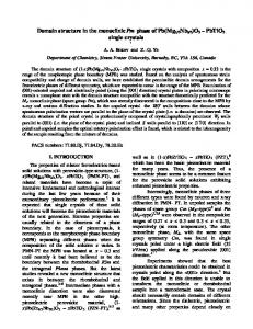
3.1 Distribution of obstacle strengths Forest dislocations are non-extended obstacles whose interactions are effective over a few atomic distances only, and can therefore be idealized as point obstacles. Pairs of such point obstacles arrest dislocations, which require a certain threshold resolved shear stress s to overcome the barrier, Fig. 1. The value of s can be estimated from line tension calculations, see for example Kovács and Zsoldos (1973). The simplest such estimate gives

s=

b l

(20)

where is the shear modulus, b the length of the Burgers vector, l the length of the link, and a numerical coefficient of the order of : (Kuhlmann-Wilsdorf, 1989). For simplicity, we start by assuming that all forest dislocation intersections give rise to obstacles of the same strength, regardless of the precise nature of the interaction. This assumption is relaxed in Section 4. Since the distribution of point obstacles within the glide plane is random, it follows that s itself is a random variable. We shall let f s; t denote the probability density function of two-point barrier strengths at time t. The time dependence of f s; t is a consequence of the variation in forest dislocation density. If, for simplicity, the locations of the point obstacles are assumed to be completely uncorrelated, and assuming further that the pairs of points defining a barrier are next neighbors, it follows that (Kocks, 1966)

03

~( ) ~( )

f~(l; t) = 2n(t)l exp( n(t)l2 )

(21) where n(t) is the area density of forest dislocation intersections with the glide plane at time t, andf~(l; t) is

the probability density function for next neighbor distances. Using (20) to effect a change of variables from l to s, we arrive at " #

2n(t)(b)2 exp f~(s; t) = s3

The corresponding distribution function is computed to be

P~ (s; t) = exp

"

n(t)

n(t)

b 2 s

b 2 # s

~( )

(22)

(23)

Direct measurements of f l; t were made by Mughrabi (1975), and by Grosskreutz and Mughrabi (1975). The ability of (21) to fit the data is quite remarkable. Modeling and Simulation in Material Sciences and Engineering, 1:(3),pp. 225–263.

Cuitiño & Ortiz


FINAL

7

τ

INITIAL

Fig. 1. Schematic representation of a dislocation passing through a random distribution of point obstacles under the action of a monotonically increasing resolved shear stress .

3.2 Kinetics of dislocation motion Next we turn to the interaction between a moving dislocation line and the distribution of point obstacles. Our discussion here is restricted to the analytically tractable case of rate-independent behavior and monotonic loading. A more general theory which accounts for rate-sensitivity effects and arbitrary loading paths has been given by Ortiz and Popov (1982). Thermal effects can be included into the theory by recourse to models of thermally activated dislocation motion such as those advanced by Teodosiu and Sidoroff (1976). Let t be the resolved shear stress acting on the slip system at time t. Assume for now that t increases monotonically from zero at t . Evidently, for dislocations to be stable at time t they must face t dt, the dislocation segments held barriers of strengths s in excess of t . As t is increased to t t dt are dislodged and move forward until they at barriers of strengths in the range t s t t dt, Fig. 1. This motion of dislocations results in an incremental reach barriers of strength s t increase in the plastic deformation. In the rate-independent formulation, the dislocation jumps between obstacles are assumed to be instantaneous. This idealization is justified for quasistatic loading, when the duration of the flights is much smaller than the characteristic time of variation of the loads. As noted by Ortiz and Popov (1982), the information needed to describe the dislocation motion is fully contained in the probability density function f s; t , which represents the fraction of dislocation length facing barriers of strength s at time t. This is, therefore, the primary unknown of the theory. The function f s; t evolves in time due to the process of redistribution of dislocation line described above. Initially, though, the dislocations may be assumed to be randomly distributed over their slip plane, and

()

()

=0 () () ( ) + _( ) () ( ) + _( ) ( ) + _( ) ( )

( )

f (s; 0) = f~(s; 0):

( )

0

(24)

()

At later times, f s; t must vanish identically for s < t in the rate-independent limit. Next, we endeavor to determine a kinetic equation for the evolution of f s; t . Consider a time increment dt over which the applied resolved shear stress is incremented by an amount t dt, with t . Then, t dt become the dislocation segments facing barriers of strengths in the interval t s t t dt. The probability that an unstable unstable and move to stronger barriers of strengths s > t

( ) + _( )

()

( ) _( )

_( ) 0 ( ) + _( )


Cuitiño & Ortiz


8

dislocation segment moves to a barrier of strength s0 is given by

f~(s0 js0 > (t)) =

f~(s0 ; t)H (s0 (t)) 1 P~ ( (t); t)

(25)

where H is the Heaviside step function. Thus, the displaced dislocation segments redistribute themselves proportionally to f s0 ; t over the admissible interval t ; 1 . Consequently, the transition probability that a dislocation segment moves from a barrier of strength s to another of strength s0 is f s0 js0 > t Æ s t t dt, and the correponding transition probability rate is

~( )

[ () )

( )) _ ( )

~(

0 ~ 0 (s ! s0; t) = f (s1; t)HP~ ((s(t); t)(t)) Æ(s

( )) (

(t))_ (t)

(26)

Because of the Markovian nature of the dislocation flights, the evolution of f master equation (see, e. g., Résibois & de Leener 1977)

(s; t) is governed by Pauli’s

@f (s; t) @t

( )

=

Z1 0

[ (s0 ! s; t)f (s0; t)

(s ! s0; t)f (s; t)]ds0 + g(s; t)

(27)

( ) ( )

where g s; t is a source term which describes the rate of variation of f s; t due to external agencies and in the absence of transitions. For the system under consideration, g s; t represents the rate of change of f s; t due to the evolution of barrier strength probabilities f s; t . As noted earlier, this latter evolution is in turn caused by variations in the density of forest dislocations n t , e. g., through (22). To evaluate g s; t we view t as frozen at its current value and suppose that f s; t changes into f s; t dt , i. e., we regard all dislocation segments as stably pinned at their current locations, while pointobstacles are added or removed from the slip plane. Some of the new obstacles pin down the dislocation lines and, consequently, a change in f s; t results. The probability that a segment comes to face a newly formed barrier of strength s is proportional to f s; t , over the admissible range t ; 1 . Therefore, the rate at which f s; t changes due to this mechanism is

~( ) ()

( )

( )

~( + )

()

( )

( )

g(s; t) =

@ @t

~( )

~( )

"

[ () )

#

1

f~(; t) H (s ) P~ (; t) = (t)

(28)

where the notation implies that the time derivative is to be carried out at constant . Inserting (26) and (28) into (27) the sought equation of evolution for f s; t is found to be

@f (s; t) @t

=

"

f~(s; t)H (s (t)) 1 P~ ( (t); t)

Æ(s (t))

#

@ f ( (t); t)_ (t)+ @t

"

( ) f~(; t) 1 P~ (; t) H (s

)

# = (t)

(29)

_( ) 0

where it is implicitly understood that t . Eq. (29) may be viewed as a statement of gains and losses. Indeed, the Dirac-delta term on the right hand t dt, while the side has the effect of removing probability density from the interval t s t remaining term in the bracket distributes it over the admissible interval t ; 1 proportionally tof s; t , Fig. 2.

() ( ) + _( ) [ () )


~( )

Cuitiño & Ortiz


9

f(s,t)

. τ(t) dt

s

τ(t)

( )

_ (t)dt.

Fig. 2. Redistribution of the probability density f s; t upon a resolved shear stress increment The third term represents a probability source term, as discussed in the foregoing. We note that

Z 1 @f (s; t) @t

0

ds = 0

(30)

which, together with (24), insures that the normalization condition

Z1 0

f (s; t)ds = 1

(31) () = 0

0

is satisfied at all times. A noteworthy limiting case of (29) is obtained when t , t , i. e., when the slip system remains unloaded at all times. In this case, it follows immediately from (29) that f s; t f s; t , t . That this should indeed be the case follows from the fact that, in the absence of applied stress, the dislocation lines remain randomly distributed over the slip plane and, consequently, the probability that a segment face a barrier of strength s is necessarily equal tof s; t . Remarkably, kinetic equation (29) admits the simple closed form solution

( ) = ~( )

0

~( )

f (s; t) =

f~(s; t)H (s (t)) 1 P~ ( (t); t)

(32)

This probability density function is readily verified to satisfy (29) by direct substitution. Again, it should be emphasized that (32) is valid for monotonically increasing t only. The case of general loading is considerably more complex (Ortiz and Popov, 1982). Solution (32) implies that, under the conditions of the analysis, the probability density f s; t remains proportional to f s; t over the current admissible range t ; 1 . The various stages of the evolution of f s; t are shown in Fig. 3, for the case in which f s; t and P s; t are given by (22) and (23), respectively. As will be demonstrated subsequently, (32) fully characterizes the self-hardening of a slip system.

[ () ) ~( )

( )

( )

() ~( )


~( )

Cuitiño & Ortiz


10

1.20

1.00

τ / τc 0.

f(s/τc)

0.80

0.6 0.8

0.60

1.0 0.40

1.2 1.4

0.20

0.00 0.0

1.0

2.0

Fig. 3. Probability density f

s / τc

3.0

4.0

5.0

(s; t) for different values of =c.

3.3 Plastic strain rate

_( )

()

Next we proceed to calculate the slip rate t induced by the dislocation motion. Let t denote the current dislocation length per unit volume for the slip system under consideration. t varies in time according to kinetic equations formulated in Section 4. The dislocation density released during an increment of the t dt gives rise to an incremental plastic strain (Kocks, 1966; resolved shear stress from t to t Teodosiu, 1970)

()

()

( ) + _( ) d (t) = b(t)f ( (t); t))_ (t)dtN (t)l(t); (33) (t) is the average number of jumps the dislocation where l(t) is the average distance between barriers, and N

segments make before attaining stable positions, Fig. 4.

s

∆τ

τ

X

l N l

Fig. 4. 1-D schematic representation of a dislocation segment moving through random obstacles. The dislocation segment is initially trapped at an obstacle of strength s . After a resolved shear stress . increment is applied, the segment glides until it is trapped again at a new obstacle of strength s

+


Cuitiño & Ortiz


( )

To a good approximation, l t can be identified with the average distance hli For f l; t as in (21), this gives

( )

11

(t) between point obstacles.

l(t) = hli(t) = p1 (34) 2 n(t) (t). Evidently, the probability that an unstable segment Next we compute the average number of jumps N becomes arrested after the first jump is equal to the probability that the first barrier encountered is of a strength s (t). This probability is 1 P~ ( (t); t). The probability that the segment goes beyond the first barrier is P~ ( (t); t). Likewise, the probability that a segment gets arrested at the second barrier encountered is P~ ( (t); t)[1 P~ ( (t); t)], and the probability that it goes beyond is P~ 2 ( (t); t), and so on. Hence, the

average number of jumps between barriers taken by an unstable segment is

N (t) = [1 P~ ( (t); t)]+2P~ ( (t); t)[1 P~ ( (t); t)]+3P~ 2 ( (t); t)[1 P~ ( (t); t)] =

=0

1 ~ 1 P ( (t); t) (35)

Interestingly, if , any moving dislocation segment is sure to be arrested at the first obstacle it encoun, in agreement with (35). Likewise, if f s; t has a bounded support, say ; smax t , and ters, and N t > smax t , then the segment never reaches a stable barrier and N ! 1, as predicted by (35). Substituting (35) and (32) with s + t into (33) we finally obtain

()

=1 ()

~( )

[0

( )]

= () f~( (t); t)

_ (t) = c(t) (36) [1 P~ ( (t); t)]2 _ (t) where the characteristic plastic strain c (t) is defined as

c (t) = b(t)l(t) (37) It bears emphasis that (36) is explicit in f~(s; t) and (t). The former is given by (22) and (23), once the point obstacle density n(t) is known. This, in turn, is a function of the dislocation densities in the remaining slip systems. The precise form of this dependence is discussed in Section 4.

3.4 Self-hardening As expected from the rate-independent character of the formulation, (36) defines a relation of the form

_ (t) =

_ (t) h(t)

(38)

(t) is the self-hardening modulus of the slip system. In view of (36) one has, explicitly, 1 = c(t) f~( (t); t) (39) h(t) [1 P~ ( (t); t)]2 As before, this formula is valid for any assumed distribution f~(s; t) of barrier strengths. If, for instance, we take f~(s; t) to be given by (22), then (39) becomes 2 2 3 (t) c (t) h(t) = hc (t) 3 cosh 1 (40) (t) 2 (t) where h

c

p

where

c(t) = b n(t);

hc (t) =

c(t)

c (t)

(41)

are a characteristic shear stress and plastic modulus, respectively. Eq. (40) predicts an initial infinite hard. The hardening modulus subsequently decreases monotonically to zero as is ening modulus at increased. The values of c and c determine the location of the ‘bend’ in the resolved shear stress-slip strain curve. Thus, c correlates with the value of the flow stress determined by backextrapolation.

=0


Cuitiño & Ortiz


12

3.5 Elastic unloading and rate effects In the present rate-independent framework, the above relations can be extended simply to account for loading histories exhibiting elastic unloading. Thus, we no longer assume that the loading is monotonic, but continue to require that t not change sign throughout the loading history. Define the current flow stress g t of the slip system as

()

()

g(t) =

In rate form,

()

g_ (t) = _ (t); 0;

max (s)

(42)

s2[0;t]

( ) = (t) and _ (t) 0;

if t g otherwise.

(43)

Thus, g t is defined to be the maximum attained resolved shear stress on the slip system. if t < g t . Thus, Because f s; t vanishes in the interval ; g t , it follows from (33) that t the interval ; g t acts as an induced elastic domain: any part of the loading history contained in ; g t leaves (and g ) unchanged. The same is true of loading increments such that t g t but t . . Physically, the stability of the dislocations in the glide system requires Note that in this latter case g t that they all be pinned at obstacles of strength greater or equal to the previously maximum attained resolved shear stress g t . Therefore, subsequent stresses in the range ; g t are not capable of causing further dislocation motion. Under these conditions (38) and (39) are to be rewritten as

( ) [0 ( ))

[0 ( )]

_( ) = 0 ( ) ()= ()

_( ) = 0

()

() [0 ( )) _( ) = 0

[0 ( ))

_ (t) =

g_ (t) ; h(t)

1 = c(t) f~(g(t); t) h(t) [1 P~ (g(t); t)]2

(44)

In is evident from (43) that the first of (44) incorporates the loading-unloading criteria appropriate to nonmonotonic loading. The preceding analysis can be generalized to the case in which the dislocation jumps between obstacles are not instantaneous but occur at a speed which is a function of the resolved shear stress (Ortiz and Popov, 1982). Unfortunately, the resulting master equation (27) cannot be solved in closed form. Phenomenologically, however, rate effects can be readily built into the constitutive description by adopting a power viscosity law of the form (15). Mathematically, the resulting formulation can be regarded as a viscoplastic regularization of the rate-independent relations.

4 CROSS-HARDENING The preceding section has been concerned with the statistics of the motion of a dislocation line through dislocations intersecting its plane, or forest dislocations. The ensuing short-range interactions determine the rate of self-hardening of a slip system in the present theory. A key variable in the description of the selfhardening of, say, system is the density n of point obstacles afforded by forest dislocations. Evidently, n is a function of the dislocation densities in all remaining systems. The experimental work of Franciosi and co-workers (Franciosi et al., 1980; Franciosi and Zaoui, 1982; Franciosi, 1983, 1985a, 1985b, 1988) is suggestive of a dependence of the form X n a

=

(45)

Experimentally determined values of the interaction matrix a have been given by Franciosi and Zaoui directions in FCC (1982) for the twelve slip systems belonging to the family of f g planes and and f g in BCC crystals, and by Franciosi (1983) for the twenty-four systems of types f g crystals.

111

211 [111]

[110]


110 [111]

Cuitiño & Ortiz


13

They classify the interactions according to whether the dislocations belong to the same system (interaction coefficient a0 ), fail to form junctions (interaction coefficient a1 ), form Hirth locks (interaction coefficient a1 ), co-planar junctions (interaction coefficient a1 ), glissile junctions (interaction coefficient a2 ), or sessile Lomer-Cottrell locks (interaction coefficient a3 ), with a0 a1 a2 a3 . Franciosi (1985) has also found the interaction coefficients to be linearly dependent on the stacking fault energy of the crystal, the degree of anisotropy increasing with decreasing stacking fault energy. It bears emphasis that the statistical analysis given in Section 3 is predicated on the simplifying assumption that all point obstacles on a slip plane are of equal strength. However, the strength of point obstacles, as measured by the coefficient in (20), may be expected to be a strong function of the type of threading dislocation (Baird and Gale, 1965). A rigorous treatment of obstacle strength distribution effects necessitates a substantial modification of the statistical analysis given in Section 3 (see, e. g., Friedrichs and Haasen, 1975). In a more phenomenological vein, it is possible to lump and n together in eq. (41) and account for obstacle strength variations through the coupling matrix a a` la Franciosi. In order to obtain a closed set of constitutive relations, equations of evolution for the dislocation densities are required. Processes resulting in changes in dislocation density include production by fixed sources, such as Frank-Read sources, breeding by cross-glide and pair annihilation (see Kuhlmann-Wilsdorf, 1989, for a recent review). The operation of fixed Frack-Read sources, however, usually stops after inducing a relatively small amount of plastic deformation. Consequently, production by fixed sources, while sometimes important during the early stages of plastic deformation, is quickly eclipsed by production due to cross-glide and can be safely neglected. The importance of breeding by cross-glide as a dislocation generation mechanism was emphasized by Johnston and Gilman (1959,1960). In this mechanism, the screw section of a moving dislocation migrates to a parallel plane by cross-slip, thus creating a pair of immovable jogs. The ends of the jogs act as the fixed points of single-ended plane sources. Theoretical (Li, 1961) and experimental (Johnston and Gilman, 1959, 1960) investigations suggest that the breeding rate due to cross-glide is proportional to the mean dislocation speed. This gives the relation b

_ = _

(46)

for the rate of dislocation generation due to cross-glide multiplication. The coefficient may be interpreted as the reciprocal mean free path between cross-glide events. The rate of pair annihilation is proportional to the probability of having two dislocations segments of opposite sign in a small neighborhood of each other, and, thus, may be expected to be roughly proportional to the dislocation density squared (Sackett et al. 1976). The average time between encounters is inversely proportional to the mean dislocation speed. Consequently, the rate of dislocation attrition due to pair annihilation can be expressed as (Sackett et al. 1976) b

_ =

_

(47)

where may be regarded as the mean radius of interaction for segment annihilation. Combining (46) and (47), the total rate of change of dislocation density may be written in the suggestive form (Gillis and Gilman, 1965; Essmann and Rapp, 1973)

_ =

b

1

_ sat

(48)

where sat = is a saturation density at which the rate of annihilation balances the rate of production. Eq. (48) defines a linear ordinary differential equation for of solution

= sat 1

1

0 sat

e

= sat


(49)

Cuitiño & Ortiz


14

where sat bsat = is a saturation shear strain, 0 is the initial dislocation density in system , and we . It bears emphasis that relation (49) places the dislocation density and the have assumed that slip strain in one-to-one correspondence. It should be carefully noted that we do not differentiate explicitly between mobile and immobile dislocation densities. In the above expressions, is used to denote the total (i. e., mobile and immobile) dislocation density. At any time during the deformation process, the fraction of the dislocation density which contributes to the plastic strain rate is determined by the probability density function f s; t introduced in the preceding section. Since (48) involves , the right hand side is implicitly proportional to the mobile dislocation fraction.

(0) = 0

_

( )

_

5 SUMMARY OF CONSTITUTIVE RELATIONS For ease of reference, the relations defining the dislocation model are collected in Box 1. Box 1. Hardening relations

1=m 1] if > g ) = _ 0 [( =g ) 0 otherwise. g g_ 3 =( h _" 2 # ) h = hc cosh gc 1

_ (

; g

hc =

c ;

c

c p c b n ; X n a

= sat 1

=

1

0 sat

c

e

= sat

2

b p

n

Remarkably, the dislocation-based model outlined in Box 1 conforms to the general structure suggested by Bassani and Wu (1989) on the basis of their own experimental data. Specifically, the matrix h entering the hardening relations (16) is predicted to be diagonal. The precise way in which latent hardening is predicted to occur by the dislocation model is as follows. During the initial single slip regime, dislocation multiplication takes place predominantly on the primary slip system. Hence, the number of point obstacles ). and the deformation proceeds by on the primary system remains relatively small (constant if a easy glide. At the same time, the number of point obstacles on the secondary systems grows rapidly due to dislocation multiplication on the primary system, with rates determined by the influence coefficients a . This has the effect of raising the values of the reference, or ‘critical’, stresses c on the secondary systems. Consequently, despite the fact that the yield stress g remains small on the secondary systems, the reloading curve in a latent-hardening experiment simulation rises steeply above the primary loading curve, as observed experimentally (e. g., Kocks, 1970). A detailed comparison between theory and latent-hardening data is presented in Section 7.2. The correspondence between the dislocation model and that of Pierce et al. (1983) can be made more apparent by computing c from (41), (45) and (48). As noted earlier, c correlates with the flow stress

=0

_


Cuitiño & Ortiz


_

15

_

obtained by back-extrapolation. A simple calculation shows that c and are linearly related as

_ =

c

X ^

h

h^ =

_

;

^

c 2n a b

sat

1

(50)

Evidently, the hardening matrix h is non-diagonal. Initially, when the dislocation densities are low on all systems, the ordering a a results in the off-diagonal terms of h being dominant. It should be noted, however, that the hardening matrix h is not constant but depends strongly on the deformation history. It may therefore be concluded that some of the discrepancies between the various theories regarding the form of the hardening matrix stem largely from the definition of flow stress adopted. If, as in the Piece et al. model, the emphasis is placed on c , which roughly corresponds to a back-extrapolation definition of the flow stress as in (Kocks, 1970), then the corresponding hardening matrix is nondiagonal. If, on the contrary, the variation of the yield stress, or elastic limit, is sought, as in the model of Bassani and Wu (1989), then a diagonal hardening matrix becomes appropriate. The dislocation model outlined in the foregoing shows that these two views are complementary, rather than contradictory.

^

^

6 NUMERICAL IMPLEMENTATION Next we turn our attention to matters of numerical implementation of the foregoing models in the context of implicit finite element computation. Implicit finite element methods applied to elastoplastic solids can prove advantageous in applications in which the stress and deformation paths remain nearly proportional. Under these conditions, implicit methods can significantly speed up the calculations by enabling the use of larger time steps than otherwise permitted by their explicit counterparts. Even if the global equilibrium equations are handled explicitly, it is often advantageous to perform the local updates implicitly, since implicit updates add considerable robustness to the calculations and rid them of the exacting constraints placed by stability in the nearly rate-independent limit. Implicit methods which seek to exactly satisfy equilibrium, compatibility and some suitable state-update rule at every load increment were formalized by Hughes and Taylor (1978) for the viscoplastic solid, and by Simó and Taylor (1985) for the rate-independent solid. A Newton-Raphson solution of the resulting incremental nonlinear equations requires the formulation of so-called ‘consistent tangents’ (Simó and Taylor, 1985) obtained by direct linearization of the state-update algorithm. Here we focus on the backward-Euler or fully implicit method and show how the local update can be reduced to a nonlinear system of equations for the incremental slip strains. The jacobian matrix of the system can be derived explicitly, which enables the efficient computation of the incremental slip strains by a local Newton-Raphson iteration. We also give the consistent tangents for the algorithm explicitly in closed form. A difficulty which arises in the context of crystalline plasticity concerns the determination of the active slip systems under conditions of multiple slip. We define an iterative procedure for determining the pattern of slip activity which reduces to the conventional elastic-predictor plastic-corrector implementation of implicit updates for solids with a single yield surface.

6.1 Consistent tangents In a Newton-Raphson solution of the governing equations (4), the linearized problem for the incremental displacements takes the form

Z

B0

r0 : K^ n+1 : r0u dV0 forcing terms = 0


(51)

Cuitiño & Ortiz


where the ‘consistent tangents’

K^ n+1 follow by linearization of the stress update (2) as ^ K^ n+1 @ F@ P (Fn+1 ; state at tn; 4t) n+1

16

(52)

Alternatively, the linerized virtual work principle (51) can be expressed in spatial form as

Z

B0

r : k^ n+1 : ru dV0 forcing terms = 0

where r is the spatial gradient operator and the spatial consistent tangents

kîjkl = K^ iJkL FjJ FlL

k are defined as

(53) (54)

Whereas for small strains the computation of the consistent tangents reduces to a straightforward exercise for many commonly used models, for finite deformation formulations the calculations are considerably more cumbersome. It is, therefore, quite remarkable that in the case of single crystals the consistent tangents can be written down explicitly with some generality, as shown next.

6.2 State update All the models discussed above, namely, the models of Pierce et al. (1983), Section 2.2, Bassani and Wu (1989), Section 2.3, and the dislocation model developed in the preceding sections, conform to the general constitutive framework summarized in Box 2, which also shows the corresponding backward-Euler time discretization. Box 2. State Update Algorithm

Constitutive : F= Fe Fp ; C e = FeT FPe; F_ pFp 1 = _ s m ; S = S (C e); es)T S m ; = (C

_ = P ( ; g ); g_ = h ( )_ ;

(Fpn+1

Incremental : p e Fn+1 = Fn+1 Fn+1 C enP+1 = FeTn+1Fen+1 Fpn)Fpn+11 = 4 s m S n+1 = S (C en+1) en+1s )T S n+1m n+1 = (C 4 P = 4t(n+1 ; gn+1) 4g = h ( n+1)4

For convenience, we have collected all slip strains in an array . Sums on or extend over the currently active slip systems, which for now we shall presume known. A procedure for determining the set of active slip systems is given in Section 6.4. The algorithm in Box 2 defines a nonlinear system of equations which can be solved for the updated state as a function of n+1 and the initial conditions for the increment. A convenient method of solution consists of reducing the system to a set of equations for 4 . This may be accomplished as follows. To avoid the numerical ill-conditioning which results from the frequently adopted power-law form of , we begin by inverting the discretized viscosity law and rewriting it as n+1 4 =4t; gn+1 In this equation, gn+1 is a function of 4 through the hardening law. In addition, using the relations in Box 2 n+1 can be written as a function of en+1 which, in turn, can be expressed in terms of 4 using the discretized flow rule. Thus, (55) defines a system of equations of the form f 4 n+1 4 =4t; gn+1

F

= (

)

(55)

C

( )=

(

)=0


(56)

Cuitiño & Ortiz


17

This system can now be solved by a Newton-Raphson iteration. A lengthy but straightforward computation yields the required jacobian matrix @f =@ 4 explicitly. The resulting convergence rate is quadratic and convergence is typically achieved to within machine precision in two or three iterations.

(

)

6.3 Explicit expression for the consistent tangents The consistent tangents (54) for the update algorithm listed in Box 2 can be computed in closed form. A trite calculation yields e kîjkl = kijkl

XX

where

e r )(n C e ) A 1 (Cijmn mn pq pqkl

A =

XX

1 Æ + n C e

ij ijkl rkl

4t

h~ = h + nij =

@

X @h

@

+ r )(n C e ) A 1 (in rjn jn in pq pqkl

(57)

@ ~ h @g

(58)

4

F e 1F e 1 @ S IJ Ii Jj F e 1F e 1 rij = R IJ Ii Jj

(59) (60) (61) (62)

p 1 e s m P R ij = CIK K L (Fn )LA FAJ e = @ SIJ F e 1 F e 1 F e 1 F e 1 Cijkl (63) Ii Jj Kk Ll e @ CKL e are the spatial and we have dropped the subindex n +1 from all updated quantities. In these definitions Cijkl

n

r

elastic moduli and and play the role of effective spatial normal and plastic flow direction, respectively. As expected from general results on finite plasticity (see, e. g., Moran et al. 1990), the consistent tangents (57) are generally unsymmetric. The use of a set of exact tangents ensures a quadratic asymptotic rate of convergence of the global equilibrium iterations. In order to increase the radius of convergence of the Newton-Raphson iteration, it is often convenient to perform line searches to scale the incremental displacements. Practical line search methods are reviewed by Crisfield (1991).

6.4 Determination of the active slip systems In the foregoing discussion the set of active slip systems has been presumed known. In a typical calculation, the pattern of slip activity changes with deformation and the active set has to be continuously updated. We define the active set L as the set of systems such that n+1 > gn+1 . The flowchart of an iterative algorithm for determining the active set is given in Box 3. Box 3. Determination of Active Systems i) Initialize L

= ;.

ii) Compute 4 based on current L. iii If 4

< 0 remove from L, set 4 = 0. Modeling and Simulation in Material Sciences and Engineering, 1:(3),pp. 225–263.

Cuitiño & Ortiz


18

vi) Update remaining state variables based on current 4 . v) Is n+1

gn+1 8 not in L?.

NO: Add most loaded system(s) (i. e., maximum n+1

gn+1 ) to L;

GO TO (ii).

YES: EXIT. Evidently, the starting iteration of the algorithm corresponds to an elastic update. For single yield surface models, the search stops after at most an additional iteration, and the algorithm reduces to the conventional elastic-predictor/plastic-corrector implementation of implicit updates. If a largely stable set of active systems is anticipated for a given loading path, it may prove advantageous to replace the default initialization, L ;, to the set of active systems from the previous converged solution, whereupon the searching algorithm converges in one iteration for as long as the slip pattern remains unchanged.

=

6.5 Adaptive meshing Plastic regions in crystals are often narrow and elongated, and extend along well-defined crystallographic directions. The slip patterns induced by cracks in single crystals are a case in point, as demonstrated by the numerical simulations presented in Section 8. Under these conditions, the velocity field and other aspects of the solution exhibit a rapid variation across the plastic zones while varying slowly in other directions. In cases where the geometry of the evolving fields is not known a priori, adaptive meshing techniques furnish an effective device for resolving the fine structure of the solution. For the applications discussed in Section 8, an adaptation criterion based on the equidistribution of plastic work has proven useful. In this approach, elements with a plastic work contents exceeding a prescribed tolerance T OL, i. e., elements such that

Z

eh

W pd > T OL

are targeted for refinement. Here, eh denotes the domain of element density W p is given by Zt X p W dt

=

0

(

(64) e and, for crystals, the plastic work

_ )

(65)

Clearly, this criterion leads to refinement in regions of high plastic deformation. In simulations involving cracks subjected to monotonically increasing loads (cf. Section 8), the plastic work equidistribution criterion results in continuous generation of elements at the tip and enables the mesh to track the expanding plastic regions. A remeshing technique for finitely deforming plastic solids has been proposed by Ortiz and Quigley (1991). In Ortiz and Quigley’s (1991) approach, meshes consisting of six-noded triangular elements with three quadrature points and constant pressure are constructed by Delaunay triangulation (Sloan, 1987). The connectivity of the mesh is determined from the set of corner nodes of the elements, with the midnodes added subsequently. The mesh is adapted at regular intervals by adding new corner nodes at the midsides of elements targeted for refinement. The element connectivity is then completely redefined by a Delaunay triangulation based on the new set of corner nodes. In particular, no hierarchical compatibility between subsequent meshes is enforced. After each triangulation, Crane et al.’s (1976) implementation of Gibbs et al.’s (1976) bandwidth minimization algorithm is applied. Finally, a variationally consistent transfer operator proposed by Ortiz and Quigley (1991) is used to transfer the state variables between meshes following an adaptation. Modeling and Simulation in Material Sciences and Engineering, 1:(3),pp. 225–263.

Cuitiño & Ortiz


19

The plastic work equidistribution criterion is amenable to an error minimization interpretation in some simple cases. To illustrate this connection, consider the case of a solid deforming in antiplane shear relative to the x1 x2 plane. Let the solid obey J2 -deformation theory of plasticity with power-law hardening. The equation governing the out-of-plane displacement u x1 ; x2 is

(

r (j ru j 2 ru) = f;

) in u = 0;

on @

(66)

= ( + 1)

where n is the hardening exponent, n =n and, for simplicity, we assume homogeneous Dirichlet boundary conditions. Under suitable restrictions on the forcing f , an appropriate solution space for u is the (e. g., Oden et al., 1986). Under these conditions, the plastic work in element e is Sobolev space W01; given by the energy seminorm, i. e.,

( )

Z

eh

W pd =

1 j ue j

(67)

h W 1; ( e ) 0 h

where ueh is the finite element solution over element eh . Therefore, in this case equidistributing plastic work is equivalent to equidistributing the energy over the mesh. This affords an illuminating connection between plastic work equidistribution and the interpolation error method of Diaz et al. (1983). Let ueh be the interpolant over eh derived from the nodal values of u. Let k and m be integers and p; q 2 ; 1 be numbers such that Wk+1;p eh is contained in W m;q eh with a continuous injection. Let the interpolation functions in eh include the complete set of polynomials up to order k . Then (Ciarlet, 1978), there exists a constant C such that, for all ue 2 W k+1;p eh ,

0

~

0

[1 ]

( )

( )

(he )k+1 Ehe jue u~eh jm;q; eh C [meas( eh )]1=q 1=p e m jue jk+1;p; eh ( )

meas( )

( )

(68)

e is the measure of e and e the diameter of the largest ball where ue is the restriction of u to eh , h h e contained in h . The requisite continuous injection condition is satisfied if (Ciarlet, 1978)

1=1 q

p

k+1 m ; d

k+1 m
g , i. e., when the resolved shear stress on the system exceeds its yield stress. The simulations reported here are performed using a single 8-node brick finite element. The tensile direction is aligned with the element axes. The two loaded faces of the cube are constrained to remain parallel to each other and perpendicular to the loading axis. These boundary conditions simulate a stiff loading device in which the clamps are prevented from rotating. The values of the material constants employed in the calculations are listed in Table I. Table I. Material constants. Elastic Constant C11 : 3 MPa Elastic Constant C12 : 3 MPa Elastic Constant C44 : 3 MPa g0 : MPa

_ 0 m b

sat 0 sat a0 a1 =a0 a2 =a0 a3 =a0

168 4 10 121 4 10 75 4 10 20 1 sec 1 0:01 0:3 2:56 10 10 m 0:5% 1012 m 2 1015 m 2 75 10 5 5:7 10:2 16:6

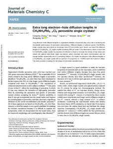
7.1 Multislip tests Fig. 5 shows a comparison between theoretical and experimentally determined uniaxial tension stress-strain curves for copper single crystals. The experimental data is taken from Franciosi and Zaoui (1982). With the notable exception of the [001]-[111] zone axis, the experimental record shows that the majority of high symmetry tensile directions result in substantial amounts of single slip prior to the inception of multiple glide. Even for the [001]-[111] zone axis, however, the relative extents of plastic activity in the various slip systems vary in time, with different combinations of systems dominating the early and late stages of deformation depending on the orientation of the tensile axis.


Cuitiño & Ortiz


150

150

125

125 100

σ [MPa]

100

111

σ [MPa]

21

75

001 112

50

111 75

001

50

112

012

122

25

0 0.000

25

122 011 0.025

0.050

0.075

0.100

0.125

012

0 0.000

0.150

011 0.025

0.050

0.075

0.100

0.125

0.150

ε

ε

Fig. 5. Uniaxial tension test for copper single crystals. a) Experimental measurements, (Franciosi and Zaoui, 1982); b) dislocation model. Our numerical simulations are indicative of a very high sensitivity of the behavior of the crystal to small misalignments of the loading axis. Small deviations of the axis (< Æ from its nominal direction give rise to variations in the pattern of slip activity and to substantial quantitative differences in the predicted stress-strain curves. This high sensitivity may partly account for the considerable scatter in experimental stress-strain curves obtained under nominally identical conditions, Fig. 5. The sensitivity to misalignments of the loading axis is particularly acute for high symmetry orientations of the crystal.

1)

0.250

100

D1

A3

Exprimental Data 0.150

γ

σ [MPa]

75

0.200

Numerical Simulation

50

σ,ε

A6

0.100

D6

Tensile Axis 112

25

0.050

B4 0 0.000

0.050

0.100

ε

0.150

0.200

0.250

40

0.000 0.000

0.100

0.150

0.200

0.250

ε 1000

A3

D1

D1

30

A3

B4

A6 D6

750

D6

ρ / ρ0

A6

τ [MPa]

0.050

20

B4

500

B2 10

C1

B2

250

C3 D4 A2

0 0.000

0.050

0.100

0.150

ε

0.200

B5 0.250

C1 0.000

0.050

0.100

0.150

0.200

C3

0.250

ε

Fig. 6. Tensile axis [112]. a) Stress-strain curve; b) slip strains; c) resolved shear stresses, and d) dislocation densities. Fig. 6.a compares theoretical vs. experimental (Franciosi and Zaoui, 1982) stress-strain curves for a crystal loaded in uniaxial tension in the [112] direction. A good overall agreement between the two sets of curves is evident from the figure. Due to a small misalignment in the loading axis intentionally introduced


Cuitiño & Ortiz


22

in the simulations, system D1 yields first. 2 Here and subsequently, we adhere to the standard Schimdt and Boas convention for designating the slip systems of an FCC crystal. During the early stages of deformation, deformation, the additional system A3 is easy glide by single slip on system D1 is predicted. At about activated, and an attendant upturn in the stress-strain curve is observed. An upturn of this type is commonly identified with the inception of the stage II of hardening. The variation of the relevant slip strains with deformation is shown in Fig. 6.b The ranges of deformation where single and multiple slip are dominant are clearly identifiable in the figure.

3%

60

perfect orientation

σ [MPa]

40

20 error along [001]-[111] zone axis error between [001]-[111] & [001]-[011] zone axes error along [001]-[011] zone axis

0 0.000

0.050

0.100

ε

Fig. 7. Theoretical stress-strain curves for various misalignments of the [001] tensile axis. The precise manner in which small misalignments of the loading axis produce large variations in the response bears some emphasis. For uniaxial loading in the [112] direction, the resolved shear stresses on systems A3 and D1 are identical under nominal conditions. However, in our numerical simulation the axis misorientation causes yielding in system D1 to occur slightly in advance of its nominal inception point, Fig. 6.c. The exponential dislocation multiplication law (49) then produces a precipitous increase in the obstacle density on all other systems, Fig. 6.d, with an attendant rapid rate of hardening as measured by c , eq. (41). Eventually, the resolved shear stress on A3 reaches the yield level, which has hitherto remained near its initial value. With the ensuing slip, A3 hardens and its resolved shear stress remains close to that ), of D1, Fig. 6.d. Interestingly, although some plastic activity on A3 is recorded during stage I ( < the resulting slip strains are negligible in this range when compared to those on D1. In this sense, D1 is overwhelmingly dominant and the crystal may be regarded as undergoing single slip. When the saturation : is attained, Fig. 6.b, the rate of dislocation multiplication on D1, and the rate of slip strain sat hardening on all other systems, slow down considerably. This allows A3, and other systems subsequently, to become active, thus bringing the single slip regime to an end.

3%

0.0500

0.0500

0.0450

0.0450

0.0400

0.0400

0.0350

0.0350

0.0300

0.0300

0.0250

0.0250

γ

γ

= 0 5%

0.0200

0.0200

0.0150

0.0150

0.0100

A2 D4 C1 C3

0.0050 0.025

0.050

ε 2

A3 D1

0.0100

A3 A2 B2 B4 C1 C3 D1 D4

0.0050 0.0000 0.000

B2 B4

0.075

0.100

0.0000 0.000

0.025

0.050

0.075

ε

*


0.100

Cuitiño & Ortiz


0.0500

0.0500

0.0450

0.0450

0.0400

0.0400

B4 A3 0.0300

0.0300

0.0250

0.0250

0.0200

0.0200

0.0150

0.0150

C3 D4

A2 B2

0.0100 0.0050 0.025

0.050

A3

B4

0.0350

γ

γ

0.0350

0.0000 0.000

23

B2 D4 A2 C3

0.0100

D1

C1 D1

0.0050

C1

0.075

0.0000 0.000

0.100

0.025

ε

0.050

0.075

0.100

ε

Fig. 8. Slip strains, [001] tensile axis. a) Pefect alignment of the loading axis; b) misalignment along the [001]-[111] zone axis; c) misalignment between the [001]-[111] and [001]-[011] zone axes; and d) misalignment along the [001]-[011] zone axis. In summary, two main mechanisms are responsible for the single-multiple slip transition. The first factor is geometrical in nature, and concerns the small variations in resolved shear stress between nominally identical systems introduced by slight misalignments of the loading axis. Indeed, simulations based on a mathematically exact orientation of the crystal predict simultaneous slip on all nominally active systems and fail to exhibit a stage I-stage II transition. By itself, a misorientation of the loading axis would not be sufficient to cause large variations in the behavior of the crystal were it not for the exponential growth capable of being sustained by the dislocation densities prior to saturation. The rapid pace of dislocation multiplication in the system which yields earliest causes the remaining nominally active systems to harden, thus delaying their activity. 20

20

15

15

τ [MPa]

τ [MPa]

C1 C3 A2 D4

A3 A2 B2 B4 C1 C3 D1 D4 10

5

0 0.000

A3 D1 B2 B4

10

5

0.025

0.050

0.075

0 0.000

0.100

0.025

ε

0.050

0.075

0.100

ε

20

20

C3 D4 15

τ [MPa]

τ [MPa]

15

A2 B2 C1 D1

A3 B4 10

5

0 0.000

C3 D4 A2 C1 B2 D1 A3 B4

10

5

0.025

0.050

ε

0.075

0.100

0 0.000

0.025

0.050

0.075

0.100

ε

Fig. 9. Resolved shear stresses, [001] tensile axis. a) Pefect alignment of the loading axis; b) misalignment along the [001]-[111] zone axis; c) misalignment between the [001]-[111] and [001]-[011] zone axes; and d) misalignment along the [001]-[011] zone axis. Modeling and Simulation in Material Sciences and Engineering, 1:(3),pp. 225–263.

Cuitiño & Ortiz


24

The misorientation sensitivity in the response of the crystal is exacerbated in situations where the loading axis coincides with a direction of high symmetry. To illustrate this effect, next we consider the configuration of highest possible symmetry, namely, a [001] tensile axis. For this orientation, eight slip systems are potentially active. We have considered four orientations of the tensile axis differing by less than : Æ : a) a mathematically exact [001] tensile axis; b) a misalignment along the [001]-[111] zone axis; c) a misalignment between the [001]-[111] and [001]-[011] zone axes; and d) a misalignment along the [001]-[011] zone axis. Fig. 7 compares the predicted stress-strain curves. A wide spread in the results is clearly apparent, with the stiffest response occurring for the perfectly aligned axis. During the early stages of deformation, the rate of hardening is also highest in the perfectly oriented crystal. Subsequently, the hardening rates become ostensibly identical in all cases.

05

1000

1000

A3 A2 B2 B4 C1 C3 D1 D4

750

ρ / ρ0

ρ / ρ0

750

500

250

B2 B4

A3 D1

500

0.025

0.050

0.075

0.100

0.000

0.025

0.050

ε

0.100

1000

A3 B4

C3 D4

A2 B2

750

C1 D1

ρ / ρ0

ρ / ρ0

0.075

ε

1000

500

250

0.000

C1 C3

250

0.000

750

A2 D4

B4

B2

A3

D4

C3 A2

C1 D1

500

250

0.025

0.050

ε

0.075

0.100

0.000

0.025

0.050

0.075

0.100

ε

Fig. 10. Dislocation densities, [001] tensile axis. a) Pefect alignment of the loading axis; b) misalignment along the [001]-[111] zone axis; c) misalignment between the [001]-[111] and [001]-[011] zone axes; and d) misalignment along the [001]-[011] zone axis. The discrepancies in the patterns of slip activity are even more pronounced, Fig. 8. Under nominal conditions, all eight potentially active systems yield simultaneously, Fig. 8.a. For the misoriented crystals, the activity of some systems is significantly delayed, Figs. 8.a, 8.b and 8.c. In all cases, the slip activity is consistent with the symmetries preserved by the misalignment of the axis. By way of example, in case (b) the pairs of systems B2-B4, A3-D1, A2-D4 and C1-C3 slip by the same amount. As expected, all eight systems exhibit different slip activities in case (d), in which no symmetries are preserved. The causes underlying the observed variations in the response of the crystal with misorientation are similar to those noted in the case of loading in the [112] direction. As is evident from Fig. 8, the slip activity in the most loaded systems has the effect of inhibiting slip in the remaining systems up until saturation. Remarkably, despite the wide disparity in slip activities the resolved shear stress and hardening rate remain nearly the same in all systems, Fig. 9, as required by equilibrium. It is interesting to note that, owing to the high symmetry of the loading axis, the lattice rotations remain small at all times. The lag introduced


Cuitiño & Ortiz


25

by misorientation in the activity of certain systems is also evident in Fig. 10, which shows the evolution of dislocation densities. The most loaded systems exhibit rapid growth initially and then quickly saturate. At this point, their inhibiting effect on the remaining systems stops. The increased activity in these systems accounts for the sudden upturn in their rate of dislocation multiplication, Fig. 10.

7.2 Latent-hardening tests In latent-hardening tests, secondary flow stresses are determined from the reloading stress-strain curve by backextrapolation. A shortcoming of this procedure is that, because the reloading curves need not tend to a straight asymptote, the measurements are sensitive to the offset shear strain chosen. Therefore, comparisons between theory and experiment must necessarily be qualitative in nature. Latent hardening data is often reported in terms of the latent hardening ratio LHR s =p , where p and s denote the flow stresses of the primary and secondary slip system, respectively. Fig. 11 shows theoretical plots of the LHR as a function of the prestrain p on the primary system and the strength of the interaction between the primary and secondary systems, as measured by the coefficients ai , Section 4. In keeping with the experimental procedure, the computed values of the flow stresses are obtained from the reloading stressstrain curve by backextrapolation to s . Theory and experiment are in good qualitative agreement as is a direct consequence regards the dependence of the LHR on prestrain. The initial value of the LHR of its definition and of the fact that, for an FCC crystal, the initial flow stress in a well-annealed crystal is the same in all systems. The LHR subsequently goes through a maximum and then settles down to a value which remains nearly constant under increasing prestrain. The mechanisms underlying this dependence bear some interest. In the prestraining stage, the variation of s is determined by dislocation multiplication on the primary system and the attendant increase in the density of point defects on the secondary system. By contrast, the variation of p in the same stage solely reflects the self-hardening of the primary system. Because of the exponential growth in dislocation density on the primary system, for small prestrains s attains values considerably in excess of p , and hence the initial precipitous increase in the LHR with prestrain, Fig. 11. For prestrains such that p sat , the dislocation density on the primary system saturates and s attains a nearly constant value. At the same time, p continues to grow slowly due to self-hardening on the primary system, and a downturn in the LHR- p curve ensues, Fig. 11.

=

=0

=1

4.0 3.5 3.0

Medium Interaction (coefficient a2 )

LHR

2.5 2.0 1.5 1.0

Weak Interaction (coefficient a1)

0.5 0.0 0.000

0.025

γ primary

0.050

Fig. 11. Computed Latent Hardening Ratios (LHR) as a function of primary shear strain for different


Cuitiño & Ortiz


26

interaction coefficients ai . As a general rule, the stronger the interaction between primary and secondary slip systems (i. e., the larger the interaction coefficient ai ), the higher the resulting value of the LHR, Fig. 11. However, for very strong interactions, such as those described by a3 , the pattern of slip activity may deviate from that expected in latent hardening experiments, and caution must be exercised in interpreting the results. Thus, for strongly interacting systems s rises sharply over p even for small prestrains. Upon reloading, s may be so large that the primary system remains dominant. This situation tends to perpetuate itself, since the absence of any significant slip on the secondary system keeps the primary system comparatively soft and, in addition, the continuing activity of the primary system contributes to harden the secondary system further. By contrast, in cases where the primary and secondary systems interact weakly (e. g., coefficients a1 and a2 ), the secondary system slips at a rate sufficient to keep the primary system from become active during the reloading stage, as befits latent hardening experiments. These predicted differences in behavior for varying interaction strengths are in full agreement with the observations of Franciosi and Zaoui (1982).

8 NUMERICAL SIMULATION OF CRACKS IN SINGLE CRYSTALS Calculations of near-tip fields in single crystals provide an example of application of the methodology described in previous sections. The specific boundary value problem analyzed is that of a crack on the plane of a copper single crystal, with the crack front in the direction, and crack growth along , Fig. 12. Combinations of slip systems which result in plane-strain deformations are pairs of the type and , which jointly give rise to effective in-plane shear along the direction, Fig. 13. and combine to produce effective in-plane slip along the Similarly, the systems direction. Finally, the pair of systems and operating jointly also result in plane-strain deformations. The small-strain yield surface corresponding to this case is shown in Fig. 14.

[101]

[110]

(111) [011]

(111) [110]

(111) [011] (111) [101] (111) [101]

[121]

X2-[010] CRACK PLANE

[100] X1-[101] [001] CRACK FRONT

X3-[101]

Fig. 12. Crack on

(010) plane in a FCC crystal with the crack front parallel to [101].


(010) [101] (111) [121]

Cuitiño & Ortiz


[110]

27

[011] [011]

CRACK PLANE

(111)

[110]

-

(111) CRACK FRONT

-

(111) CRACK PLANE

-

(111) [101]

CRACK FRONT

Fig. 13. Slip systems capable of producing sustained plane strain plastic deformations. The finite deformation case has proven intractable by analytical means and has to be dealt with numerically. Fig. 15 shows the initial finite element mesh used in the computations. We have chosen to round the tip of the crack into a circular notch or root-radius r0 , Fig. 15.a. The initial mesh is fan-like, and divides the upper half plane into 8 equal sectors centered at the tip, Fig. 15.b. The ratio of the radius of the remote boundary R to the notch root radius is 4 . The crack opening is driven by prescribing the anisotropic K -field displacements on the remote boundary. The crack is loaded up to a maximum value of elastic p K= g0 R . At this point, the root-radius of the notch has expanded by , and the maximum slip strains are of the order of 3 times the initial yield strain. Intentionally, the initial mesh is too coarse to adequately resolve the solution. To provide the requisite resolution, we resort to the adaptive meshing technique described in Section 6.5. The final mesh is shown in Fig. 16. The value of the plastic work contents at : 7 . The calculations are based which an element is targeted for refinement is T OL= r02 g02 =C44 on the dislocation model described in Section 5. The material constants adopted in the analysis are listed in Table I.

10

(

)=5

20%

10

(

) = 1 5 10

τ12 √3

√(3/2)

(τ11 - τ22)/2

Fig. 14. Small-strain yield surface for an FCC crystal with the orientation shown in Fig. 12 undergoing plane strain deformation. The following terminology proves helpful in interpreting the results of the calculations. For cracks


Cuitiño & Ortiz


28

loaded in mode I, plastic shearing on the most active slip systems can occur either parallel or perpendicular to the active slip planes. Shearing parallel to slip planes, or shear mode, is accommodated by edge dislocations emanating from the crack-tip. Thus, in the shear mode, the crack tip itself acts as dislocation source. By way of contrast, shearing perpendicular to the slip planes, or kink mode, necessitates the formation of dislocation dipoles (Cahn, 1951). The activation of this mode requires abundant internal sources of dislocation emission. Kink modes of deformation involve extensive lattice rotations, which may in turn induce geometric hardening or softening depending on the direction of rotation (Asaro, 1983).

Fig. 15. Initial mesh containing 256 six-node triangular elements). a) Close-up view of the near-tip region; b) overall view of the mesh.

Fig. 16. Final mesh containing 2700 elements Fig. 17 shows the computed isocontours of slip activity in the small-strain region away from the crack and at Æ ; ii) a kink tip. The dominant slip modes are three: i) a shear mode on Æ Æ and at ; and iii) a shear mode at on and . mode on The variation of the components of the Kirchhoff stress tensor and the slip strains with the polar angle is shown in Figs. 18.a and Fig. 18.b, respectively. It is clear from these figures that the three dominant slip modes determine directions of rapid variation of displacements and stresses. The adaptive meshing procedure effectively provides adequate mesh resolution in those regions.

(111) [101]

(111) [101] 90

(111) [011] (111) [110] 55 145 (111) [110] (111) [011]


Cuitiño & Ortiz


(111) [101] and (111) [101]

γ 1.0E-3 6.3E-4 4.0E-4 2.5E-4 1.6E-4 1.0E-4 6.3E-5 4.0E-5 2.5E-5 0.0E0

(111) [110] and (111) [011]

γ 1.0E-3 6.3E-4 4.0E-4 2.5E-4 1.6E-4 1.0E-4 6.3E-5 4.0E-5 2.5E-5 0.0E0

(111) [110] and (111) [011]

γ 1.0E-3 6.3E-4 4.0E-4 1.6E-4 1.0E-4 6.3E-5 4.0E-5 2.5E-5 1.6E-5 0.0E0

Fig. 17. Isocontours of slip strain in the small-strain region away from the crack tip.


29

Cuitiño & Ortiz


8.00

30

0.00060

6.00

τ22

4.00

τ11

Numerical Solution Analytical Solution (Rice, 1987)

(111)[110] and (111)[011]

(111)[101] and (111)[101]

0.00050

τij / g0

(111)[110] and (111)[011] 0.00040

γ

0.00030

2.00 0.00020

0.00

τ12

0.00010

-2.00

0.00000 0

30

60

90

θ

120

150

180

0

30

60

90

θ

120

150

180

Fig. 18. Variation of: a) the components of the Kirchhoff stress tensor; b) the slip strains, as a function of the polar angle at r : R Fig. 19 shows the isocontours of slip activity at closer range to the crack tip. The slip pattern changes as a result of the emergence of two additional kink modes: one on system at Æ ; and a second Æ . As is evident from Figs. 20.a and 20.b, the slip strains and stresses vary slowly at mode on with in this region. Consequently, the adaptation procedure gives rise to a less structured mesh.

= 0 18

(111) [121] 40

(111) [121] 170

( (111) [101] and (111) [101]

γ 1.0E-3 6.3E-4 4.0E-4 2.5E-4 1.6E-4 1.0E-4 6.5E-5 4.1E-5 2.5E-5 1.6E-5 0.0E0

(111) [110] and (111) [011]

γ 1.0E-3 6.3E-4 4.0E-4 2.5E-4 1.6E-4 1.0E-4 6.3E-5 4.0E-5 2.5E-5 1.6E-5 0.0E0


Cuitiño & Ortiz


31

(111) [110] and (111) [011]

γ 1.0E-3 6.3E-4 4.0E-4 2.5E-4 1.6E-4 1.0E-4 6.3E-5 4.0E-5 2.5E-5 1.6E-5 0.0E0

Fig. 19. Isocontours of slip strain in the vicinity of the crack tip.

28.00

0.0200

24.00

0.0175

τ22

20.00

0.0150

(111)[110] and (111)[011]

16.00

τij / g0

(111)[110] and (111)[011]

(111)[101] and (111)[101]

0.0125 12.00

τ11

γ

8.00

0.0100 0.0075

4.00 0.0050

0.00

τ12

-4.00

0.0025

-8.00

0.0000 0

30

60

θ

90

120

150

0

30

60

90

θ

120

150

180

Fig. 20. Variation of: a) the components of the Kirchhoff stress tensor; b) the slip strains, as a function : R of the polar angle at r

= 0 001

9 DISCUSSION Cracks in single crystals have been investigated by Rice and Nikolic (1985) and Rice (1987) within the framework of small-strain ideal plasticity, and by Rice and Saeedvafa (1988) and Saeedvafa and Rice (1989), who also restricted their analysis to small strains and no lattice rotations but allowed for Taylor, or isotropic, power-law hardening. Mohan el al. (1992a and 1992b) subsequently analyzed cracks of the same geometry by means of a geometrically rigorous formulation which accounted for finite lattice rotations. The calculations where based on the formulation of Pierce et al. (1983), and on a phenomenological hardening law proposed by Chang and Asaro (1981) for Al-Cu alloys (cf. Section 2.3). The crystals described by this law exhibit a first stage of rapid hardening followed by ideally plastic behavior. This is in sharp contrast to the stage I-stage II structure of the hardening of single-phase FCC crystals. For some orientations, the results of Mohan el al. (1991) differ from the predictions of the small-strain theory, but are in good overall agreement with the experimental observations of Shield and Kim (1990). These analyses, together with the simulations described in Section 8, illustrate the strong influence of the kinematic assumptions and the details of the hardening law on solutions to specific boundary value problems.


Cuitiño & Ortiz




τ12/τM 1.0

τ12/τM 1.0

0.5 -2.0

-1.0

0.5 2.0

1.0 θ = 180

θ=0

32

(τ11- τ22)/2τM

-2.0

-1.0

2.0

1.0 θ = 180

θ=0

-0.5

-0.5

-1.0

-1.0

-1.5

-1.5

-2.0

-2.0

= 0 18

(τ11- τ22)/2τM

= 0 001

Fig. 21. Trajectory of the Kirchhoff stress in the at: a) r : R; b) r : R. Rice (1987) gave an analytical solution to the problem considered in Section 8 under the assumption of small strains and lattice rotations and ideal rigid-plastic behavior. Rice (1987) additionally assumed that the solid was everywhere at yield, so that the stresses were constrained to lie on a fixed hexagonal yield surface 12 stress plane, Fig. 14. Under these conditions, Rice (1987) obtained an analytical in the 11 22 = solution by piecing together four sectors of constant stress and double slip. These sectors were separated by three radial lines of displacement and stress discontinuity representing narrow regions of single slip. The : Æ support shear modes on and , while the rays of discontinuity at : Æ and Æ to the plane of crack corresponds to a kink mode on and . Fig. discontinuity at 21.a shows the trajectory obtained in the stress plane by sampling the solution on a semicircle centered at the tip, with varying between the limits and , corresponding to the half-plane following the crack and the upper crack face, respectively. The stress -trajectory effects a half turn around the yield surface. Evidently, the numerical solution given in Section 8 agrees closely with Rice’s (1987) solution in the outer section of the plastic zone, Fig. 18. This owes to the fact that, in that region, strains and lattice rotations are small and the crystal deforms by easy glide, which can be idealized as perfectly plastic behavior to a good approximation. These are precisely the conditions under which Rice’s (1987) solution applies. Closer to the tip, the crystal enters the stage II of hardening. This stage is characterized by strong interactions between the slip systems and by rapid hardening. The computed slip strain variation with polar angle is depicted in Fig 20. A noteworthy feature of the slip pattern is the presence of triple glide sectors. This is in contrast with the structure of the solution in the easy glide region, which consists of sectors of single and double glide only. This limitation is peculiar to Taylor or isotropic hardening models such as those considered by Rice (1987) and Saeedvafa and Rice (1989), for which the yield surface is constrained to remain undistorted. Fig. 21.b shows the computed -trajectory in Kirchhoff stress space normalized by the resolved shear stress M in the most active slip system. The stress trajectory nearly effects a full turn around the origin. It bears emphasis that the calculations predict all of the solid to be at yield. The results of Mohan et al. (1991) provide a noteworthy counterpoint to the above picture. Because of the hardening law adopted in their computations, the crystal exhibits a rapid rate of hardening in the small-strain region away from the crack tip. Since, in addition, hardening was assumed to be isotropic, the calculations of Mohan et al. (1991) are reminiscent of the high hardening limit of Saaedvafa and Rice’s solution (1988) in that region. Closer to the crack tip, the crystal no longer hardens and Rice’s (1987) solution might be anticipated to become dominant. Instead, the calculations differ substantially from the

(

)2

90

54 7

(211) [111] (211) [111] (011) [111] (011) [111]

125 3

0


Cuitiño & Ortiz


(211) [111] 112 (211) [111]

33

40

analytical solution of Rice (1987). Thus, the system gives rise to a kink mode at Æ , and a less Æ . A less intense kink mode at Æ and an even weaker shear mode at Æ are intense shear mode at system. Finally, slip on the system gives rise to a shear mode contributed by the at about Æ to the plane of the crack. Finite lattice rotations, which are neglected in Rice’s analysis, may account for these discrepancies. Indeed, the calculations reveal the presence of substantial lattice rotations which tend to concentrate in the direction of the kink modes. The axis of lattice rotation is nearly uniform throughout the crystal and parallel to the crack front. Finite rotations of the lattice may induce geometrical hardening or softening (Asaro, 1983), depending on the direction of rotation. Localization instabilities induced by geometrical softening may in turn have a marked influence on the prevailing deformation pattern (Asaro and Rice, 1977). These effects cannot be properly accounted for unless finite deformations and, specifically, finite lattice rotations are rigorously included in the formulation. Interestingly, the calculations of Mohan et al. (1991) are in good agreement with the experimental observations of Shield and Kim (1990) on Fe-Si crystals, which attests to the adequacy of the modelling for this class of materials.

70

130 (011) [111]

22

ACKNOWLEDGEMENTS The support of the U. S. Office of Naval Research through grant N00014-90-J-1758 is gratefully acknowledged. MO is grateful for support received while on visit at the LPMTM of the Universite Paris Nord, where some aspects of the work reported in this paper were partly completed. MO is also indebted to P. Franciosi for many helpful discussions.

REFERENCES 1. Ambrosi P., Göttler, E. & Schwink Ch. 1974. On dislocation arrangement and flow stress of [111] cooper single crystals deformed in tension, Scripta Metall., 8, p. 1093. 2. Asaro, R. J. 1983. Micromechanics of crystals and polycrystals, Adv. Appl. Mech., 23, p. 1. 3. Asaro, R. J. & Rice, J. R. 1977. Strain localization in ductile single crystals, J. Mech. Phys. Solids, 25, p. 309. 4. Baird, J. D. & Gale, B. 1965. Attractive dislocation intersections and work hardening in metals, Phil. Trans. Roy. Soc., A257, p. 553. 5. Bassani, J. L. & Wu T. Y. 1989. Latent hardening in single crystals: Part 2. Analytical characterization and predictions, University of Pennsylvania. 6. Bassani, J. L. 1990. Single crystal hardening, Appl. Mech. Rev., 45, p. 320. 7. Cahn, R. W. 1951- Slip and polygonization in aluminum, J. Inst. Metals, 79, p. 129. 8. Chang, Y. W. & Asaro, R. J. 1981. An experimental study of shear localization in aluminum-copper single crystals, Acta Metall., 29, p. 241. 9. Ciarlet P. G. 1978. The Finite Element Method for Elliptic Problems, North-Holland. 10. Crane H. L., Jr., Gibbs N. E., Poole W. G., and Stockmeyer P. K. 1976. Matrix Bandwidth and Profile Reduction, ACM-CALGO Algorithm 508, ACM Trans. Math. Software, 2 p. 375. 11. Crisfield, M. A. 1991. Non-Linear Finite Element Analysis of Solids and Structures, Vol. 1, Wiley. Modeling and Simulation in Material Sciences and Engineering, 1:(3),pp. 225–263.

Cuitiño & Ortiz


34

12. Devloo P., Oden J. T., and Strouboulis T. 1987. Implementation of an adaptive refinement technique for the SUPG algorithm, Comp. Meth. Appl. Mech. Engng., 61 p. 339. 13. Diaz A. R. ,Kikuchi N., and Taylor J. E. 1983. A method of grid optimization for finite element methods, Comp. Meth. Appl. Mech. Engng., 41, p. 29. 14. Essmann, U. & Rapp, M. 1973. Slip in copper crystals following weak neutron bombardment, Acta Metall., 21, p. 1305. 15. Foreman, A. J. E. & Makin, M. J. 1966. Dislocation movement through random arrays of obstacles, Phil. Mag., 14, p. 911. 16. Foreman, A. J. E. & Makin, M. J. 1967. Dislocation movement through random arrays of obstacles, Canadian J. Phys., 45, p. 511. 17. Franciosi, P., Berveiller, M. & Zaoui, A. 1980. Latent hardening in copper and aluminium single crystals, Acta Metall., 28, p. 273. 18. Franciosi, P. & Zaoui, A. 1982. Multislip in F. C. C. crystals: A theoretical approach compared with experimental data, Acta Metall., 30, p. 1627. 19. Franciosi, P. 1983. Glide mechanisms in B. C. C. crystals: and investigation of the case of -iron through multislip and latent hardening tests, Acta Metall., 31, p. 1331. 20. Franciosi, P. 1985a. The concepts of latent hardening and strain hardening in metallic single crystals, Acta Metall., 33, p. 1601. 21. Franciosi, P. 1985b. FCC single crystals hardening: anisotropy and stacking fault energy, Proc. ICSMA Symp., Montreal, Canada, p. 281. 22. Franciosi, P. 1988. On flow and work hardening expression correlations in metallic single crystal plasticity, Revue Phys. Appl., 23, p. 383. 23. Friedrichs, J. and Haasen, P. 1975. Ternary solution-hardening of copper single crystals, Phil. Mag., 31, p. 863. 24. Gibbs N. E., Poole W. G., Jr., and Stockmeyer P. K. 1976. An Algorithm for Reducing the Bandwidth and Profile of a Sparse Matrix, SIAM J. Numer. Anal., 13 p. 235. 25. Gillis, P. P. & Gilman, J. 1965. Dynamical dislocation theory of crystals plasticity. II. Easy glide and strain hardening, J. Appl. Phys., 36, p. 3380. 26. Grosskreutz, J. C. & Mughrabi H. 1975. Description of the work-hardened structure at low temperature in cyclic deformation, in: A. S. Argon (ed.), Constitutive Equations in Plasticity, Cambridge:MIT Press, p. 251. 27. Havner, K. S. 1973. On the mechanics of crystalline solids, J. Mech. Phys. Solids, 21, p. 383. 28. Hill, R. & Rice, J. R. 1972. Constitutive analysis of elastic-plastic crystals at arbitrary strain, J. Mech. Phys. Solids, 20, p. 401. 29. Hughes, T. J. R. and Taylor, R. L. 1978. Unconditionally stable algorithm for quasi-static elasto visco-plastic finite element analysis, Comp. Struct., 8, p. 169. Modeling and Simulation in Material Sciences and Engineering, 1:(3),pp. 225–263.

Cuitiño & Ortiz


35

30. Johnston, W. G., and Gilman, J. J. 1959. Dislocation velocities, dislocation densities and plastic flow in lithium flouride crystals, J. Appl. Phys., 30, p. 129. 31. Johnston, W. G., and Gilman, J. J. 1960. Dislocation multiplication in lithium flouride crystals, J. Appl. Phys., 31, p. 632. 32. Kocks, U. F. 1960. Polyslip in single crystals, Acta Metall., 8, p. 345. 33. Kocks, U. F. 1964. Latent hardening and secondary slip in aluminum and silver. Trans. Metall. Soc., AIME, 230, p. 1160. 34. Kocks, U. F. 1966. A statistical theory of flow stress and work-hardening, Phil. Mag., 13, p. 541. 35. Kocks, U. F. 1970. The relation between polycrystal deformation and single-crystal deformation, Metall. Trans., 1, p. 1121. 36. Kocks, U. F. & Brown T. J. 1966. Latent hardening in aluminum, Acta Metall., 14, p. 87. 37. Kovács, I. & Zsoldos, L. 1973. Dislocation and plastic deformation, Pergamon Press. 38. Kuhlmann-Wilsdorf, D. 1989. Theory of plastic deformation: properties of low energy dislocation structures, Matls. Sci. Engng., A113, p. 1. 39. Lee, E. H. 1969. Elastic-plastic deformation at finite strains, J. Appl. Mech., ASME, 36, p. 1. 40. Li, J. C. M., 1961. Cross slip and cross climb induced by a locked dislocation, J. Appl. Phys., 32, p. 593. 41. Mandel, J. 1972. Plasticité classique et viscoplasticité, Lecture Notes, Int. Centre for Mech. Sci., Udine, Berlin: Springer. 42. Marsden, J. E. & Hughes, T. J. R. 1983. Mathematical Foundations of Elasticity, Englewood Cliffs: Prentice-Hall. 43. Miura, S., Kuriyama, Y. & Yoshitaka, S. 1977. Deformation behavior of single crystals, Trans. Japan Inst. Metals, 18, p. 852.

oriented copper

44. Mohan, R., Ortiz, M., and Shih, C. F. 1992a. An analysis of cracks in ductile single crystals: Part I Antiplane shear, J. Mech. Phys. Solids, 40, p. 291. 45. Mohan, R., Ortiz, M., and Shih, C. F. 1992b. An analysis of cracks in ductile single crystals: Part II Mode-I loading, J. Mech. Phys. Solids, 40, p 315. 46. Moran, B., Ortiz, M., and Shih, C. F. 1990. Formulation of implicit finite element methods for multiplicative finite deformation plasticity, Int. J. Num. Meth. Engr., 29, p. 483. 47. Mughrabi, H. 1975. Description of the dislocation structure after unidirectional deformation at low temperatures, in: A. S. Argon (ed.), Constitutive Equations in Plasticity, Cambridge:MIT Press, p. 199. 48. Needleman, A., Asaro, R. J., and Lemonds, J. 1985 Finite element analysis of crystalline solids, Comp. Meth. Appl. Mech. Engr., 52, p. 689.


Cuitiño & Ortiz


36

49. Oden, J. T., Demkowicz, L., Strouboulis, T., and Devloo, P. 1986. Adaptive methods for problems in solid and fluid mechanics, in: I. Babuska, O. C. Zienkiewicz, J. Gago, and E. R. de A. Oliveira (eds.), Accuracy Estimates and Adaptive Refinements in Finite Element Computations, John Wiley & Sons. 50. Ortiz, M. & Popov, E. P. 1982. A statistical theory of polycrystalline plasticity, Proc. R. Soc. Lond., A379, p. 439. 51. Ortiz, M. & Quigley, J. J., IV, 1991. Adaptive mesh refinement in strain localization problems, Comp. Meth. Appl. Mech. Engng., 90, p. 781. 52. Pierce, D, Asaro, R. J. & Needleman, A. 1983. Material rate dependence and localized deformation in crystalline solids, Acta Metall., 31, p. 1951. 53. Ramaswami, B., Kocks U. F. & Chalmers B. 1965. Latent hardening in silver and Ag-Au alloy. Trans. Metall. Soc., AIME, 233, p. 927. 54. Résibois, P. & de Leener, M. 1977. Classical Kinetic Theory of Fluids, New York: Wiley. 55. Rice, J. R. 1970. On the structure of stress-strain relations for time-dependent plastic deformation in metals, J. Appl. Mech., ASME, 37, p. 728. 56. Rice, J. R. 1971. Inelastic constitutive relations for solids: an internal-variable theory and its application to metal plasticity, J. Mech. Phys. Solids, 19, p. 433. 57. Rice, J. R., and Nikolic, R. 1985. Anti-plane shear cracks in ideally plastic crystals, J. Mech. Phys. Solids, 33, p. 595. 58. Rice, J. R. 1987. Tensile crack tip fields in elastic-ideally plastic crystals, Mechanics of Materials, 6, p. 317. 59. Rice, J. R., and Saeedvafa, M. 1988. Crack tip singular fields in ductile single crystals with Taylor power-law hardening. I: Anti-plane shear, J. Mech. Phys. Solids, 36, p. 189. 60. Sackett, J. S., Kelly, J. M. and Gillis P. P. 1976. A probabilistic approach to polycrystalline plasticity, Int. Conf. on Mech. Behav. of Mater., 2nd Proc., Boston, USA, 1, p. 28. 61. Saeedvafa, M., and Rice, J. R. 1989. Crack tip singular fields in ductile single crystals with Taylor power-law hardening. II: Plane strain, J. Mech. Phys. Solids, 37, p. 673. 62. Schwink C. & Göttler, E. 1976. Dislocation interactions, flow stress and initial work hardening of cooper single crystals with [100] axis orientation. Acta Metall., 24, p. 173. 63. Shield, T. W., and Kim, K.-S., 1990, private communication. 64. Simó, J. & Pister, K. S. 1984. Remarks on rate constitutive equations for finite deformation problems: Computational implications, Comp. Meth. Appl. Mech. Engng., 46, p. 201. 65. Simó, J. C. and Taylor, R. L. 1985. Consistent tangent operators for rate independent elasto-plasticity, Comput. Meth. Appl. Mech. Engr., 48, p. 101. 66. Sloan, S. W., 1987. A fast algorithm for constructing Delaunay triangulations in the plane, Adv. Eng. Software, 9, p. 34.


Cuitiño & Ortiz


37

67. Teodosiu, C. 1970. Proc. Conf. Fundamental Aspects of Dislocation Theory, Washington, 1969, Simmons, J. A., et al. (eds.), Natl. Bureau of Standards Special Publication, 2, p. 837. 68. Teodosiu, C. & Sidoroff, F. 1976. A finite theory of the elastoviscoplasticity of single crystals, Int. J. Engng. Sci., 14, p. 713. 69. Teodosiu, C. 1982. Elastic Models of Crystal Defects, Springer-Verlag. 70. Wu, T.-Y., Bassani, J. L. & Laird, C. 1989. Latent hardening in single crystals: Part 1. Experimental characterization, University of Pennsylvania.
