computational modelling of structures using discrete

DEPARTMENT OF CIVIL ENGINEERING SWANSEA UNIVERSITY

COMPUTATIONAL MODELLING OF STRUCTURES USING DISCRETE AND FINITE ELEMENTS

RICARDO TEIXEIRA SEPTEMBER 2009

DISSERTATION SUBMITTED TO THE SWANSEA UNIVERSITY IN CANDIDATURE FOR THE DEGREE OF DOCTOR OF PHILOSOPHY

SUMMARY The objective of this thesis is the establishment of an objective comparison between the Finite Element Method and the Discrete Element Method when modelling the mechanical behaviour of the continuum, both for quasi-static and dynamic response. These two very different approaches to the same problem have increasingly gained popularity during the last years, becoming the distinction between the fields of application of each method each time more difficult. This research aims the assessment of the accuracy of the Discrete Element Method to solve problems that traditionally belong to the field of the Finite Element Method. This comparison has the ultimate purpose of determining the applicability of the first method to problems that involve a first stage when the material is elastic or elasto-plastic, followed by a second stage where actual physical separation of portions of the material occurs. The first part of this work comprises a review of the theoretical background and numerical techniques used to solve continuum mechanics problems using the Finite Element Method, both for quasi-static and dynamic loading. A description of the Discrete Element Method, encompassing its insights and the numerical strategies involved in its implementation constitute the second part of this work. The establishment of a methodology to model the continua using a Discrete Element Method based approach, namely the development of techniques to simulate elasto-plastic behaviour and crack path modelling, accompanied by illustrative benchmark examples, are the main pylons over which the third part of this research lays.

i

DECLARATION This is to certify that this dissertation has not been previously accepted in part or in substance in candidature for any degree and is not concurrently submitted in candidature for any degree at any other University.

_______________

__________________

Candidate

Date

STATEMENT I This is to certify that except where specific reference to other investigation is made, the work presented in this dissertation is the result of the investigation of the candidate. _______________

__________________

Candidate

Date

STATEMENT II I hereby give consent for my dissertation, if accepted, to be available for photocopying and for inter-library loan, and for the title and summary to be made available to outside organizations. _______________

__________________

Candidate

Date

ii

ACKNOWLEDGEMENTS Initially, I would like to thank Professor Roger Owen for the opportunity he has given me to develop this work, always believing that in the end I would be able to “steer the boat to a safe harbour”. I would also like to thank Professor Djordje Peric for his guidance and, above all, for being a true inspiring figure that many times helped me finding the solution for many technical difficulties by simply talking to me about them.

iii

Table of Contents SUMMARY DECLARATIONS ACKNOWLEDGEMENTS TABLE OF CONTENTS

i ii iii iv

1

Introduction ............................................................................................................... 2 1.1 Summary............................................................................................................. 2

2

Continuum Mechanics ............................................................................................. 2 2.1 Introduction ......................................................................................................... 2 2.2 Eulerian and Lagrangian coordinates................................................................. 2 2.3 Deformation and motion ..................................................................................... 3 2.4 Eulerian and Lagrangian description.................................................................. 4 2.5 Displacement, velocity and acceleration ............................................................ 4 2.6 Deformation gradient .......................................................................................... 5 2.7 Strain measures.................................................................................................. 7 2.7.1 Engineering strain tensor............................................................................ 7 2.7.2 Green strain tensor ..................................................................................... 8 2.7.3 Logarithmic strain tensor ............................................................................ 9 2.8 Stress measures ............................................................................................... 10 2.8.1 Cauchy stress tensor ................................................................................ 10 2.8.2 Other stress measures ............................................................................. 12 2.8.2.1 1st Piola-Kirchoff stress tensor .............................................................. 12 2.8.2.2 2nd Piola-Kirchoff stress tensor ............................................................. 12 2.8.2.3 Kirchoff stress tensor ............................................................................ 12 2.9 Dynamic equilibrium.......................................................................................... 13 2.9.1 Translational equilibrium........................................................................... 13 2.9.2 Rotational equilibrium ............................................................................... 14 2.10 Principle of virtual work ..................................................................................... 15 2.11 Material models................................................................................................. 16 2.11.1 Linear elastic material............................................................................... 16 2.11.2 Neo-Hookean material.............................................................................. 17 2.11.3 Hencky material ........................................................................................ 18 2.12 Plasticity ............................................................................................................ 19

iv

3

FEM............................................................................................................................. 2 3.1 Introduction ......................................................................................................... 2 3.2 Finite element approximation ............................................................................. 3 3.2.1 2D Geometry and displacement ................................................................. 3 3.2.2 Strain ........................................................................................................... 8 3.2.3 Stresses ...................................................................................................... 9 3.3 Principle of Virtual Work ................................................................................... 10 3.3.1 Discretization............................................................................................. 11 3.4 Newton-Raphson solution algorithm ................................................................ 13 3.5 Finite element elasto-plasticity in small strains ................................................ 14 3.5.1 Integrating the rate equations................................................................... 14 3.6 Finite element elasto-plasticity in large strains................................................. 17 3.6.1 Multiplicative elasto-plastic kinematics..................................................... 17 3.6.2 General isotropic large strain plasticity model.......................................... 18 3.7 Consistent tangent operator ............................................................................. 19 3.7.1 Consistent tangent modulus ..................................................................... 19 3.7.2 Consistent spatial tangent modulus ......................................................... 20 3.7.3 Von Mises yield criteria ............................................................................. 21 3.8 Dynamic analysis (Time integration) ................................................................ 23 3.8.1 Introduction ............................................................................................... 23 3.8.2 Implicit and explicit time integration.......................................................... 23 3.8.3 Numerical example - Cantilever under gravity load ................................. 30

4

Discrete element method......................................................................................... 2 4.1 Introduction ......................................................................................................... 2 4.2 DEM Algorithm .................................................................................................... 3 4.3 Governing equations........................................................................................... 4 4.4 Integration in time ............................................................................................... 5 4.4.1 Leapfrog integration .................................................................................... 6 4.4.2 Time step definition..................................................................................... 7 4.5 Contact detection .............................................................................................. 10 4.5.1 Sub-division algorithm .............................................................................. 11 4.5.2 Contact forces between elements ............................................................ 14 4.5.3 Contact forces between element and boundary ...................................... 16 4.6 Contact forces................................................................................................... 18 4.6.1 Normal contact forces............................................................................... 19 4.6.2 Shear contact forces ................................................................................. 21 4.7 Examples .......................................................................................................... 22 4.7.1 Hopper feeder ........................................................................................... 22 4.7.2 “U” Channel flow ....................................................................................... 26

v

5

Discrete approach of continuum ............................................................................ 2 5.1 Introduction ......................................................................................................... 2 5.2 Discrete modelling of continuum ........................................................................ 3 5.2.1 Geometry .................................................................................................... 3 5.2.2 Contact forces............................................................................................. 5 5.3 Stress recovery ................................................................................................... 8 5.3.1 Virtual mesh generation.............................................................................. 8 5.3.2 Stress computation ..................................................................................... 9 5.4 Plasticity ............................................................................................................ 10 5.4.1 Introduction ............................................................................................... 10 5.4.2 Reduced stiffness spring model ............................................................... 10 5.5 Crack path......................................................................................................... 12 5.5.1 Introduction ............................................................................................... 12 5.5.2 Crack modelling ........................................................................................ 12 5.6 Examples .......................................................................................................... 14 5.6.1 Cantilever under gravity load.................................................................... 14 5.6.2 Cantilever under sine tip load ................................................................... 20 5.6.3 Clamped beam.......................................................................................... 24 5.6.4 “S” shape beam ........................................................................................ 29 5.6.5 Notched beam........................................................................................... 35

6

Conclusions............................................................................................................... 2 6.1 Summary of the thesis ........................................................................................ 2 6.2 Conclusions and suggestions for further research............................................. 2

vi

11 IIN NT TR RO OD DU UC CT TIIO ON N

Chapter 1. Introduction

1.1

1 Introduction 1.1

Summary

The objective of this thesis is the establishment of an objective comparison between the Finite Element Method and the Discrete Element Method when modelling the mechanical behaviour of the continuum, both for quasi-static and dynamic response. These two very different approaches to the same problem have increasingly gained popularity during the last years, becoming the distinction between the fields of application of each method each time more difficult. This research aims the assessment of the accuracy of the Discrete Element Method to solve problems that traditionally belong to the field of the Finite Element Method. This comparison has the ultimate purpose of determining the applicability of the first method to problems that involve a first stage when the material is elastic or elasto-plastic, followed by a second stage where actual physical separation of portions of the material occurs. The first part of this work comprises a review of the theoretical background and numerical techniques used to solve continuum mechanics problems using the Finite Element Method, both for quasi-static and dynamic loading. A description of the Discrete Element Method, encompassing its insights and the numerical strategies involved in its implementation constitute the second part of this work. The establishment of a methodology to model the continua using a Discrete Element Method based approach, namely the development of techniques to simulate elasto-plastic behaviour and crack path modelling, accompanied by illustrative benchmark examples, are the main pylons over which the third part of this research lays.

Chapter 1. Introduction

1.2

22 C CO ON NT TIIN NU UU UM MM ME EC CH HA AN NIIC CS S

Chapter 2. Continuum Mechanics

2.1

2 Continuum Mechanics 2.1

Introduction

Remembering that Finite Element Method lays on the continuum mechanics theories, it could not be avoided to dedicate this chapter to its the fundamental aspects as well as the ones related with what is commonly known as nonlinear continuum mechanics.

2.2

Eulerian and Lagrangian coordinates

The position vector of a material point in the reference configuration is given by

X = X iei ≡ , where

3 i =1

X iei

X. (2.1)

X i are the components the position vector, and e i are the unit base vectors of a

rectangular Cartesian coordinates system. The main feature of the vector

X is that it will not change with time. The variables X are called

material coordinates or Lagrangian coordinates. Analogously, the position vector in the current configuration is given by

x = xi e i ≡

3

i =1

xi e i


(2.2)

2.2

2.3

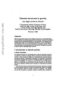
Deformation and motion

The motion of a body can be described by Belytschko (2001)

x = φ ( X, t ) or xi = φi ( X, t ) , where

(2.3)

xi = xi e i represents the position at time t of the material point X . The coordinates x

describe the spatial position of the particle are commonly known as spatial, or Eulerian coordinates. The function

φ ( X, t )

maps the reference configuration into the current configuration

at time t .

y,Y

φ(X,t)

u x

Ω0 X

Ω Γ

Γ0

x,X Figure 2.1 – Current and initial configurations of a body

If the reference configuration is identical to the initial configuration, the position vector x of any point at time t = 0 coincides with the material coordinates, hence

X = x( X,0) ≡ φ ( X,0) or X i = xi ( X,0) ≡ φi ( X,0)


(2.4)

2.3

2.4

Eulerian and Lagrangian description

Two approaches are used to describe the deformation response of a continuum. In the first approach, the independent variables are the material coordinates, X and the time t . This description is called material description or Lagrangian description. In the second approach, the independent variables are the spatial coordinates x and the time t . This is called spatial or Eulerian description. In fluid mechanics it is often unnecessary to describe the motion with respect to a reference configuration. On the other hand, in solids, the stresses generally depend on the history of deformation, forcing the use of an undeformed configuration to define the strain.

2.5

Displacement, velocity and acceleration

The displacement of a material point is given by the difference between its current position and its original position (Figure 2.1), hence

u = ( X , t ) = φ ( X , t ) − φ ( X , 0 ) = φ ( X , t ) − X , u i = φi ( X j , t ) − X i

(2.5)

The displacement can be also written as

u = x − X , ui = xi − X i

(2.6)

The velocity v ( X, t ) can be defined as the rate of change of the position vector for a certain material point, i.e. the time derivative with X held constant. These derivatives, with X held constant, are often called material time derivatives. The velocity can be expressed in many different ways as shown below.

v ( X, t ) = u =

∂φ (X, t ) ∂u(X, t ) = ∂t ∂t

In the expression above, the quantity fact that

(2.7)

x is replaced by the displacement u by using (2.6) and the

X is time independent.

The acceleration is the rate of change of velocity of a material point, which can be written as follows

a ( X, t ) =

Dv ∂v(X, t ) ∂ 2u(X, t ) =v= = Dt ∂t ∂t 2


(2.8)

2.4

2.6

Deformation gradient

As the description of deformation and measure of strain both play and essential role in nonlinear continuum mechanics, the definition of this important variable for the characterization of deformation urges. The deformation gradient is given by

F=

∂φ (X, t ) ∂xi ∂φ (X, t ) ∂x T ≡ ≡ ≡ (∇ xφ ) or Fij = i ∂X j ∂X j ∂X ∂X

(2.9)

From a purely mathematical perspective, the deformation gradient can also be defined as the Jacobian matrix of the vector function

φ (X, t ) .

y,Y F x dX

Ω

Ω0

Γ Γ0

x,X Figure 2.2 – Deformation gradient

Considering an infinitesimal line segment

dx in the reference configuration, from the (2.9) we

can see that the corresponding line segment in the current configuration is given by

dx = F ⋅ ∂X or dxi = Fij ⋅ dX j


(2.10)

2.5

The deformation gradient in a rectangular coordinate system is given by

dx1 dx1 dx1 dX 1 dX 2 dX 3 F=

dx2 dx 2 dx2 dX 1 dX 2 dX 3 dx3 dx3 dx3 dX 1 dX 2 dX 3

The determinant of

dx dX dy = dX dz dX

dx dY dy dY dz dY

(2.11)

dx dZ dy dZ dz dZ

F , commonly written as J , is known as the Jacobian determinant or the

determinant of the deformation gradient. This quantity is of most interest to relate integrals in the current and reference configurations, as follows,

f dΩ = Ω

f ( x, y, z )dxdydz =

f J dΩ 0 , or Ω0

Ω

f ( X , Y , Z )J dXdY dZ

(2.12)

Ω0

To finalize, the material derivative of the Jacobian determinant is given by

∂v DJ ≡ J = J div v ≡ J i Dt ∂xi


(2.13)

2.6

2.7

Strain measures

Unlike the linear elasticity, many different measures of strain and strain rate are used in nonlinear continuum mechanics. One of the requirements that have to be fulfilled by any strain measure is vanishing when in the presence of rigid body rotation. If a certain strain measure fails this requirement, this will mean that when undergoing a rigid body motion, this measure will predict non zero strains and consequently non zero stresses.

2.7.1

Engineering strain tensor

The Engineering strain tensor,

, gives the change in the length of the material vector,

,when comparing it with its original length,

=

dX

dx .

∂u T = (∇u ) ∂x

(2.14)

It is also common to write the Engineering strain tensor as sum of the stretch tensor and the spin tensor

=

[

] [

1 1 T T ∇u + (∇u ) + ∇u − (∇u ) 2 2 stretch tensor

]

(2.15)

spin tenso r

Using matrix notation the small strain (Engineering) tensor is given by:

εx = εx = 2γ xy

∂u ∂x ∂v ∂y

(2.16)

∂u ∂v + ∂y ∂x


2.7

2.7.2

Green strain tensor

The Green strain tensor,

E , gives the change in the square of the length of the material vector,

dX . (2.17)

ds 2 − dS 2 = 2dX ⋅ E ⋅ dX or dxi dxi − dX i dX i = 2dX i Eij dX j

The Green strain measures the difference of square of the length of an infinitesimal segment in the current (deformed) configuration and the reference (non deformed) configuration. To evaluate the Green strain tensor, we use (2.10) to rewrite (2.17) as

(

)

dx ⋅ dx = (F ⋅ dX ) ⋅ (F ⋅ dX ) = dX F T ⋅ F ⋅ dX

(2.18)

Using indicial notation, we have

(

)

dx ⋅ dx = dxi dxi = Fij dX j Fik dX k = dX j F ji Fik dX k = dX F T ⋅ F ⋅ dX Using the (2.19) with (2.17) and

dX ⋅ dX = dX ⋅ I ⋅ dX , we arrive at,

dX ⋅ F T ⋅ F ⋅ dX − dX ⋅ I ⋅ dX − dX ⋅ 2E ⋅ dX = 0 ,or

(

)

Since the relation above must hold for all

Sometimes

)

dX , we finally obtain

(

1 T 1 F ⋅ F − I or Eij = FikT Fkj − δ ij 2 2

)

(2.22)

E is written as E=

, where

(

(2.20)

(2.21)

dX ⋅ F T ⋅ F − I − 2E ⋅ dX = 0

E=

(2.19)

1 (C − I ) 2

(2.23)

C = FT ⋅ F is the right Cauchy-Green tensor.


2.8

2.7.3

Logarithmic strain tensor

The Logarithmic strain tensor,

Log

, where

=

(

Log

,is given by

)

(2.24)

1 1 ln F F T = ln(B ) 2 2

B is the left Cauchy-Green tensor.

The explicit form of this tensor is obtained performing a spectral decomposition of

B that will

yield the eigenvalues (principal stretches) and the eigenvectors (principal directions of stretching). Particularizing for the two dimensional case we have,

Log

, where

λi

=

1 ln (B ) = 2

3 i =1

1 ln (λi ) E i 2

are the eigenvalues of left Cauchy-Green tensor,

(2.25)

B , and E i are the tensors

containing the correspondent eigenprojections vectors.


2.9

2.8

Stress measures

2.8.1

Cauchy stress tensor

Let us consider a deformable body at its current position Bonet (2008).

y,Y

R2 t

∆p

n

n

∆a -n R1

-t

R1

x,X Figure 2.3 – Traction vector

The traction vector,

t , can be defined from the following mathematical limit,

∆p ∆a →0 ∆a

(2.26)

t (n) = lim

The traction vectors in Cartesian directions (stress components) (Figure 2.4) are given by e3

t (e1 ) = σ 11e1 + σ 21e 2 + σ 31e 3 t(e2 )

σ32 σ22

t (e 2 ) = σ 12 e1 + σ 22 e 2 + σ 32 e 3

(2.27)

t (e 3 ) = σ 13e1 + σ 23e 2 + σ 33e 3

Using indicial notation,

σ12 e2

e1

t (e j ) =

3 i =1

σ ij e i

(2.28)

Figure 2.4 – Stress components

The tensor

σ ij

is the Cauchy stress tensor often called as true stress due to the fact this is the

only stress measure with a physical meaning. Chapter 2. Continuum Mechanics

2.10

Lets consider the equilibrium of an elemental tetrahedron (Figure 2.5) under the action of active and passive tractions and a body force per unit of volume,

f.

e3

t(n)

t(-e ) 2

n da1

da1

da3

e1

da

e2

Figure 2.5 – Elemental tetrahedron

Writing the equilibrium equations, we have

t (n)da +

3

(2.29)

t (−e i )dai +fdv = 0

i =1

= (n ⋅ ei )da , the projection of the area, da , onto the plane orthogonal to the Cartesian direction , i

Calling dai

Dividing equation (2.29) by

da and remembering that

3

t (n ) = −

j =1

=

3 j =1

=

3 i , j =1

t(−e j )

da

j

da

t ( e j ) (n ⋅ e

j

−f

dv da

dv → 0 , we obtain, da (2.30)

)

σ ij (n ⋅ e j )e i

= σ ⋅n This Cauchy stress tensor gives the true stress acting in a facet, t , from the knowledge of the components of its normal vector,


n.

2.11

2.8.2

Other stress measures

Often within the context of finite deformations, it is more convenient to define the stress referring to a known configuration state, rather then to the real configuration state. Although these alternative stresses sometimes do not have a obvious physical meaning, they are useful as they are work conjugates of certain strain measures. st

2.8.2.1 1 Piola-Kirchoff stress tensor The 1 Piola-Kirchoff stress tensor, P , is defined as st

P = J F − tr , with J = det (F ) nd

2.8.2.2 2

(2.31)

Piola-Kirchoff stress tensor

The 2 Piola-Kirchoff stress tensor , S , is defined as nd

S = J F −1 F − tr and

(2.32)

1 F S F tr J

=

nd

We should emphasize that the 2

Piola Kirchoff stress tensor is symmetric and energetically

consistent with the Green-Lagrange strain tensor. In other words, the strain energy density calculated using the 2

nd

Piola Kirchoff stress tensor with the Green-Lagrange strain will be the

same as that calculated with the Cauchy stress tensor and the small deformation strain tensor:

= S E or

ij

ij

(2.33)

= S ij Eij

2.8.2.3 Kirchoff stress tensor The Kirchoff stress

tensor, ,

can be defined

as

the rate of

volumetric

change,

J = det (F ) ,under the time, t 0 , of a standard configuration to the time t of the current configuration.

=J

, with J = det (F )


(2.34)

2.12

2.9 2.9.1

Dynamic equilibrium Translational equilibrium

Lets consider a body under the action of body forces,

f = ρ b , and traction forces, t , per unit of

area acting on the boundary Bonet (2008). (Figure 2.6).

t

y,Y

n

φ(X,t)

dv

f v V time= t time=0

x,X Figure 2.6 – Equilibrium

The balance of linear momentum implies that

∂ ρ v dV ∂t V

= t dA + ρ b dV V

(2.35)

V

Rate of change of momentum

Remembering that

t = ⋅n ,

∂ ρ v dV = n da + ρ b dV ∂t V V V

(2.36)

Using the Gauss theorem, we obtain

ρ a dV = div dV + ρ b dV V

, where the vector

div

V

(2.37)

v

div is given by, =

3

∂σ ij

ij =1

∂x j

ei


(2.38)

2.13

The previous equation can be applied to any enclosed region of the body,

div + ρ b = ρ a

(2.39)

The equation (2.39) is known as the local spatial dynamic equilibrium equation for a deformable body. If the equation is not satisfied, (2.40) defines out of balance or residual force per unit of volume, r as:

r = div + ρ b − ρ a 2.9.2

(2.40)

Rotational equilibrium

The rotational equilibrium of general body implies that the total moment of body and traction forces about any arbitrary point, say the origin, is zero. (2.41)

x × t da + x × f dv = 0 dv

v

Remembering that the cross product of a force with a position vector,

x , yields the moment of

that force about an axis through the origin.

x × ( n ) da + x × f dv = 0 dv

(2.42)

v

After some tedious manipulation, it can be demonstrated that previous equation implies that

=

T

or

ij

=

ji

(2.43)

, which is saying that the Cauchy stress tensor is symmetric.


2.14

2.10 Principle of virtual work Let us consider a body in dynamic equilibrium and let displacements such that

δu = 0

δu be

an arbitrary set of virtual

on ΓU .

Y

ΓU δu u

Vt

Γt time= t

X

Figure 2.7 – Principle of virtual work

Multiplying the differential equilibrium equation by

δu

and integrating over the volume V . (2.44)

div δu dV + ρ b δu dV = ρ a δu dV V

v

V

Noting that

div ( δu ) = δu div + : δ and 2δ = ∇δu + (∇δu )

T

(2.45)

And using the Gauss theorem gives:

ρ a δu dV + V

: δ dV = ρ b δu dV + n δu dA V

ΓT

v

Remembering the symmetry of

and the boundary conditions:

n = t on ΓT and δu = 0 on ΓU

(2.47)

ρ a δu dV +

(2.48)

We finally have V

(2.46)

: δ dV = ρ b δu dV + t δu dA V

Work of internal forces


v

ΓT Work of external forces

2.15

Using matrix notation and defining:

[ = [σ

= ε x ε y γ xy x

]

(2.49)

T

σ y τ xy ]T

The PVW becomes:

ρ δu T u dV + δ V

T

(2.50)

dV = ρ δu T b dV + δu T b dA

V

v

ΓT

2.11 Material models 2.11.1 Linear elastic material Being this the simplest and the oldest material model, it is still one of the most essential and widely apllied in many fields of Engineering. The stress strain relation for a linear elastic material, undergoing small strains, is given by:

= D: , with

(2.51)

D , being the small strain elasticity tensor D = 2Gl + K −

2 G I⊗I 3

, defined by the Bulk modulus K , the shear modulus G , the fourth order identity tensor

(2.52)

I and

the second order identity tensor l .

E 3(1 − 2ν ) E G= 2(1 + ν ) K=


(2.53)

2.16

2.11.2 Neo-Hookean material This model, sometimes referred as the large strain extension of the Hooke’s law, is one of the simplest hyper elastic models, for moderately large deformations. The following relation between the deformation gradient,

F , and the Kirchoff stresses can be

established

= µ (B − I ) + λ ln ( J ) I ,with B = F F tr and J = det(F ) , with

(2.54)

B being the left Cauchy-Green Tensor and , F , the deformation gradient defined before.

The Lame constants

µ

and

E 2(1 + ν ) 3k − 2 µ λ= 3

λ

are given by

µ=

The real or Cauchy stresses,

= ⋅

1 J


, with k

=

E 3(1 − 2ν )

(2.55)

, can be recovered from the Kirchoff stresses as follows (2.56)

2.17

2.11.3 Hencky material The Hencky model can be defined as the finite logarithmic strain-based extension of the standard linear elastic material. This model was proposed by Hencky (1933) to model the behavior of vulcanized rubbers. Let,

Log

Log

= ln (V ) =

, be the Eulerian (spatial) logarithmic strain tensor Neto (2008). (2.57)

1 ln (B ) 2

The Hencky strain-energy function is defined in a compact form as

ρψ (

Log

)= 1

2

Log

:D:

(2.58) Log

, where D has the same format of the infinitesimal isotropic elasticity tensor referred before

2 D = 2Gl + K − G I ⊗ I 3

(2.59)

The above strain-energy renders the following linear relationship between the Kirchoff stress and the Eulerian (spatial) logarithmic strain:

=ρ

∂ψ = D: ∂


(2.60)

2.18

2.12 Plasticity Let us consider a point of a deformable body that undergoes external forces that induce deformations beyond the elastic limits of the constituent material. When this happens, part of the total deformation of the point will remain even after total unloading (Figure 2.8) and the material starts to yield entering in the plastic state.

σ σY

εp

εe

ε

ε Figure 2.8 – Uniaxial Yielding

The total strain is given by the following sum

= , where

e

and

(2.61)

e

+

p

represent the elastic (reversible) and the plastic (permanent) components of

p

the total strain.


2.19

When dealing with multiaxial states of stress, the threshold between the yielding and non yielding state (elastic and elasto-plastic) is usually defined by what is often called a yield criterion. The yield criterion is defined by a mathematical function (yield function) that depends on the existing internal stresses of the material,

σe ,

and other internal variables,

A , at certain time

step, t n . Hence,

f = f , where

σe

(

tn ,

, A, σ e

)

(2.62)

is equivalent uniaxial yield stress, commonly known as effective stress.

The yield function, f , defines the equation of a surface in the space of the principal Cauchy stresses.

σ2

a=

df dσ

σ

ELASTIC

σ

f=0 (PLASTIC)

σ1

Figure 2.9 – Multiaxial yielding

Hence, a material is yielding if the following condition is verified:

f = f

(

tn ,

)

, A, σ e = 0

(2.63)

The plastic flow is ruled by the Prandtl-Reuss flow rules translated by:

p

=λ

∂f ∂

= λa


(2.64)

2.20

, where

p

is the effective plastic strain,

a is the vector normal to the yield surface and λ is a

positive constant usually referred to as “plastic strain-rate multiplier”. The Cauchy stress changes are related to the strain via

= D( −

p

) = D(

− λa

)

(2.65)

The equation (2.65) relates mall changes in stress, and

, with small changes in elastic strain,

e

p.

For plastic flow to occur, the stresses must remain on the yield surface and hence,

f=

∂f σ = aT = a : ∂

The plastic multiplier,

(2.66)

λ , can be found we can pre multiplying equation (2.65) by a T

and using

equation (2.66).

λ=

(2.67)

aT D a:D: or λ = T a:D:a a Da

Substituting (2.64) in (2.65) we have,

= DT = D I − Where

aa T D a T Da

or

= D−

1 (D : a ) ⊗ (D : a ) : a:D:a

(2.68)

DT is the so called modular tangential matrix (or forth order tensor) which is nor only a

function of the elastic parameters ( E and

ν ) but also depends on the current Cauchy stresses,

.


2.21

References Belytschko, Ted, Liu W., Moran B. (2001)

“Nonlinear Finite Elements for Continua and Structures”, Wiley

Crisfield, M. A. (1991)

“Non-linear Finite Element Analysis of Solids and Structures - Volume 1”, Wiley


“Non-linear Finite Element Analysis of Solids and Structures - Volume 2 Advanced Topics”, Wiley

Hencky, H. (1933)

“The elastic behavior of vulcanized rubber”. Rubber Chem. Techn.6 (1933), pp. 217–224.

Neto, E. De Souza, Peric, D., Owen. D.R.J. (2008)

“Computational Methods for Plasticity – Theory and applications”, Wiley.

Bonet, J, Wood, R. D, (2008)

“Nonlinear Continuum Mechanics for Finite Element Analysis 2nd Edition” , Cambridge University Press”.


2.22

33 F FIIN NIIT TE EE EL LE EM ME EN NT TM ME ET TH HO OD D

Chapter 3. Finite Element Method

3.1

3 FEM 3.1

Introduction

Being the Finite element method a robust numerical technique to solve many different engineering problems and one of the fundamental methods in the development of this research work , it is fully justified a description of its insights. The Finite Element Method is a numerical technique that makes possible to obtain approximate solutions for the differential equations that rule most physic phenomena, including the ones related with solid mechanics. The continuum is assumed as homogeneous and often isotropic (same properties in every direction) and is divided into regions or elements. When the displacements are the unknown Zienkiewicz (2000), their values inside of the element are interpolated using special functions called Shape functions. The first part of this chapter covers the essential features of the method such as the subdivision of the domain into finite elements (discretization) and the kinematics. The aspects related with small and large strains FE plasticity are covered are discussed and explained in the following point. The last part of this chapter covers the aspects related with the techniques used to integrate the equations of motion in time, namely the commonly known as implicit and explicit methods.


3.2

3.2 3.2.1

Finite element approximation 2D Geometry and displacement

The continuum can be divided in a finite number of regions, commonly called finite elements (Figure 3.1). The set formed by these regions (elements) is called mesh. The displacement field within each element, shape functions,

u( x, y ) , can be approximated using appropriate

N i . There will be as many shape functions as the number of nodes of the finite

element possesses.

Y

ΓU

ΓU φ(X,t)

Vt V0

Γt

Mesh at time=0

Finite element

Γt Mesh at time= t

X Figure 3.1 – 2D Discretization of the continuum. Finite element mesh

These mathematical functions permit to obtain the values of a scalar field within any point of a finite element from the knowledge of the nodal values of the field. Each function,

N i , will be

worth unity at the “ i ”node of the element and zero in the remaining nodes. These same functions are often used to interpolate both the geometry and the displacement field of the problem itself. When this is the case, these finite elements are called isoparametrics.


3.3

The geometry of the element can then be interpolated as follows,

X (ξ ,η ) = Y (ξ ,η ) =

The set of axis

n i =1 n i =1

N i (ξ ,η ) X i N i (ξ ,η ) Yi

(3.1)

e

e

(ξ ,η ) are the local axis of the finite element (Figure 3.2).

(x4,y4)

Y (-1,1)

(x3,y3)

η

(1,1)

Global to local

ξ

(x1,y1)

(-1,-1)

(1,-1)

(x2,y2)

X Figure 3.2 – 2D Discretization of the continuum. Global and local coordinates

The shape functions of the four nodded quadrilateral finite element, referred to the local axis, are given by:

N 1 (ξ ,η ) =

1 (1 − ξ )(1 − η ) 4

N 2 (ξ ,η ) =

1 (1 + ξ )(1 − η ) 4

N 3 (ξ ,η ) =

1 (1 + ξ )(1 + η ) 4

N 4 (ξ ,η ) =

1 (1 − ξ )(1 + η ) 4


(3.2)

3.4

The displacement field of any point of the finite element,

u (ξ ,η ) = v(ξ ,η ) =

n i =1 n i =1

N i (ξ ,η ) ui N i (ξ ,η ) vi

u , can be obtained in a similar way, (3.3)

e

e

In the case of the four nodded quadrilateral finite element (3.2) we will have,

N1 (ξ ,η ) 0

N 2 (ξ ,η )

X(ξ ,η ) =

0 X (ξ ,η ) = N 3 (ξ ,η ) Y (ξ ,η ) 0

N 4 (ξ ,η )

0

0

N1 (ξ ,η ) 0

N 2 (ξ ,η ) 0

N 3 (ξ ,η ) 0

N 4 (ξ ,η )

x1

(3.4)

y1 x2 y2 x3 y3 x4 y4

and

N1 (ξ ,η ) 0

N 2 (ξ ,η )

u(ξ ,η ) =

0 u (ξ ,η ) = N 3 (ξ ,η ) v(ξ ,η ) 0

N 4 (ξ ,η )

0

0

N1 (ξ ,η ) 0

N 2 (ξ ,η ) 0

N 3 (ξ ,η ) 0

N 4 (ξ ,η )

u1

(3.5)

v1 u2 v2 u3 v3 u4 v4

Or, in a more compact way, we can write (3.4) as follows,

Where,

X(ξ ,η ) = N(ξ ,η ) X e

(3.6)

u(ξ ,η ) = N(ξ ,η ) u e

(3.7)

u represents the displacement vector correspondent to the local coordinates (ξ ,η ) ,

N(ξ ,η ) is the shape function matrix and u e is the vector containing the nodal displacements.


3.5

As seen in the preceding chapter on Continuum Mechanics, the measures of strain often involve the computation of partial derivatives of the displacement field,

∂u (ξ ,η ) = ∂x ∂v(ξ ,η ) = ∂x

No Nodes i =1 No Nodes i =1

u(ui , vi ) .

∂N i (ξ ,η ) ∂u (ξ ,η ) No Nodes ∂N i (ξ ,η ) ui and ui = ∂x ∂y ∂y i =1

(3.8)

∂N i (ξ ,η ) ∂v(ξ ,η ) No Nodes ∂N i (ξ ,η ) vi and = vi ∂x ∂y ∂y i =1

The derivatives of the shape functions will be obtained from the chain rule of differentiation as follows,

∂N i ∂N i ∂x ∂N i = + ∂ξ ∂x ∂ξ ∂y ∂N i ∂N i ∂x ∂N i = + ∂η ∂x ∂η ∂y

∂y ∂ξ

(3.9)

∂y ∂η

Or,

∂N i ∂x ∂y ∂ξ ∂ξ ∂ξ = ∂N i ∂x ∂y ∂η ∂η ∂η

∂N i ∂x = [J ] ∂N i ∂y

∂N i ∂x ∂N i ∂y

(3.10)

Jacobian

hence,

∂N i ∂x = J −1 ∂N i ∂y

[ ]

∂N i ∂ξ ∂N i ∂η

(3.11)

Where Ni represents shape function associated with node i of the element.


3.6

Finally, we have

∂u = ∂x ∂u = ∂y ∂v = ∂x ∂v = ∂y

n

J 11

i =1 n

−1

J 21

i =1

n

J 11

i =1 n

−1

J 21

i =1

−1

−1

(3.12)

∂N i −1 ∂N i + J 12 ui ∂ξ ∂η ∂N i −1 ∂N i + J 22 ui ∂ξ ∂η ∂N i −1 ∂N i + J 12 vi ∂ξ ∂η ∂N i −1 ∂N i + J 22 vi ∂ξ ∂η

The transformation (3.11) is valid only if the determinant of the Jacobean matrix, The elements of the Jacobean matrix of the element

∂x = ∂ξ ∂x = ∂η

n i =1 n i =1

∂N i Xi ∂ξ

∂y = ∂ξ

∂N i Xi ∂η

∂y = ∂η

n i =1 n i =1

J , is positive.

[J ] are obtained from

∂N i Yi ∂ξ ∂N i Yi ∂η

(3.13) .

The real area of the surface of the element comes from,

dA = dxdy = J dξ dη = J dξ dη . The knowledge of this area will reveal of great interest in the determination of the stiffness matrix of the element.


3.7

3.2.2

Strain

Let us consider the engineering strain tensor in Voigt notation, (3.15)

∂u ∂x ∂v ∂y

εx = εx = 2γ xy

∂u ∂v + ∂y ∂x

Remembering that the derivative of the displacement field can approximated by:

∂u = ∂x ∂u = ∂y

n i =1 n i =1

J 12

−1

J 21

−1

∂N i −1 ∂N i ui = + J 12 ∂η ∂ξ ∂N i −1 ∂N i + J 22 ui = ∂ξ ∂η

n i =1 n i =1

(3.16)

Ai ui Bi ui

We can re-write (3.13) as follows,

u1

(3.17)

v1

εx A1 0 A2 0 A3 0 A4 0 = εx = 0 B1 0 B2 0 B3 0 B4 2γ xy B1 A1 B2 A2 B3 A3 B4 A4

u2 v2 u3 v3 u4 v4

Or, in a more compact format,

= B e (ξ ,η ) U e

(3.18)

With B e , being the shape functions derivatives matrix and displacements of each degree of freedom of the element


U e the vector containing the

e.

3.8

3.2.3

Stresses

The stresses are usually computed at the same Gauss points where the numerical integration took place and they will depend upon the material model adopted. 3.2.3.1 Cauchy Stress In case of small strains, the elastic Cauchy stress in at a certain Gauss point of the element with coordinates

(ξ i ,η i ) , is given by = D = D B(ξ i ,η i ) U e

(3.19)

3.2.3.2 Kirchoff Stress Within the context of large strain plasticity, frequently becomes very useful the adoption of the Kirchoff stress tensor, . This can be easily done from the knowledge of the Cauchy stress tensor, as follows:

=J

= J D B(ξ i ,η i ) U e


(3.20)

3.9

3.3

Principle of Virtual Work

Let us consider a body in dynamic equilibrium and let

δu be

an arbitrary set of virtual

displacements such that δu = 0 on ΓU .

Y

ΓU δu u

Vt

Γt time= t

X Figure 3.3 – Discretized Principle of virtual work

Remembering the Principle of virtual work seen in Chapter 2, we have:

ρ a δu dV + V

: δ dV = ρ b δu dV + t δu dA V

(3.21)

ΓT

v


Work of external forces

With,

n = t on ΓT and δu = 0 on ΓU

(3.22)

Using matrix notation and defining:

[ = [σ

= ε x ε y γ xy x

]

(3.23)

T

σ y τ xy ]T

The PVW becomes:

ρ δu T u dV + δ V

V


T

dV = ρ δu T b dV + δu T b dA v

(3.24)

ΓT

3.10

3.3.1

Discretization

Remembering that the displacement and acceleration fields of a finite element can be approximated as

U e (x, t ) = U e (x, t ) =

n i =1 n i =1

N i (ξ ,η ) u e = N T u e (3.25)

N i (ξ ,η )u e = N u e T

And

= B e (ξ ,η ) U e

(3.26)

Substituting, we have n elem e =1

ρ δU e U e dV + δU e B e T

T

V

T

dV =

V

n elem

ρ δU e T b dV + δU e T b dA

e =1

ΓT

V


(3.27)

Work of external forces

Dividing the work into its internal and external components, we have

Wint ernal = δu e

T

Wexternal = δu e

T

n elem e =1 V


n elem e =1 V

ρ N Te N e dV u +

ρ N e T b dV +

n elem

n elem e =1 ΓT

e =1 V

T

Be

T

N e b dA

dV

(3.28)

(3.29)

3.11

Wint ernal = Wexternal for any arbitrary δu e we finally obtain the generic T

Considering that expression: n elem e =1 V

ρ N N e dV u + T e

n elem e =1 V

Be

T

dV =

n elem e =1 V

T

ρ N e b dV +

n elem e =1 ΓT

T

N e b dA

(3.30)

The previous equation can be rewritten as:

M u + FtInternal (u ) = FtExternal

(3.31)

Considering the particular case of small strain elasticity where,

= D , (3.30) will assume the

following format n elem e =1 V

ρ NTe N e dV u +

n elem e =1 V

T

B e D B e dV =

n elem e =1 V

T

ρ N e b dV +

n elem e =1 ΓT

T

N e b dA

(3.32)

Hence (3.32) can be rewritten as:

M u t + C u t + K T u t = FtExternal

(3.33)

, with the above referenced entities given by

M=

n elem e =1 V

ρ N Te N e dV

C = C(M, K ) FtExternal =

FtInternal = FtInertia = K=

n elem

ρ N e T b dV +

e =1 V n elem e =1 V

Be

n elem

n elem e =1 V

e =1 V

T

n elem e =1 ΓT

dV

ρ NTe N e dV u = M u

T

B e D B e dV

T

N e b dA

(Consistent mass matrix)

(3.34)

(Dampening matrix)

(3.35)

(External forces)

(3.36)

(Internal forces)

(Inertial forces) (Stiffness matrix)

(3.37)

or

KT =

n elem e =1 V

T

B e D T B e dV


(Tangent stiffness matrix)

3.12

3.4

Newton-Raphson solution algorithm

The solution of the linearized global equilibrium equations cannot be achieved in one single operation due to the non linear nature of the relation between the applied forces and the correspondent internal stresses. Hence, Equation (3.38) is commonly designated as a non linear system of equations in opposition to its counterpart a linear system of equations, being the last mostly restricted to the elastic small strain formulations.

M u t + C u t + K T u t = FtExternal or r = FtExternal − (FtInertia + FtInternal ) = 0

(3.38)

The Newton-Raphson algorithm consists in the following iterative scheme: 1.

Apply the target incremental load, ∆Ft +1

2.

Computation of the tangent stiffness matrix

3.

Computation of correspondent iterative displacements,

4.

Computation of the incremental displacement, du t(+i +11) = du (t +i )1 + δu (i )

5.

Computation of the associated internal and inertial forces, FtInternal and +1

6.

Computation of the residual vector,

7.

Computation of the tangent stiffness matrix

8.

Apply the residual vector, r (i +1) and norm,

9.

If

r (i +1)

= FtExternal − FtExternal +1

(

K T(i ) du t(+i )1

)

δu (i )

(

FtInertia +1

r (i ) = FtExternal − FtInternal + F+Inertia +1 +1 1t

(

K T(i+1) du t(+i +11)

)

)

r (i +1)

bigger than tolerance go to step 2 Else go to step 1

(i+2)

KT

(i+1)

Ft+1

KT

(i)

(i+2) r (i+1) r

KT

∆F

r (i)

Ft

ut

u(i)t+1

δu i

u(i+1) t+1

δu i+1

u(i+2) t+1

δu i+2

(i)

du t+1 (i+1)

du t+1

(i+2)

du t+1

Figure 3.4 – Newton-Raphson iteration scheme Chapter 3. Finite Element Method

3.13

3.5

Finite element elasto-plasticity in small strains

3.5.1

Integrating the rate equations

When solving a boundary value problem numerically, using the FEM, the stress and strain and

increments possess a finite character, hence the differentials and

will be replaced by

∆

∆ε .

By doing this we are, in fact, adding some error to the integration of the stress and strain rate equations. Hence, it is of great importance to adopt strategies that will minimize these errors. Let us consider the following figure representing the stress in a Gauss point before, after an incremental stress

∆

change has been applied,

B

=

X

X

, and

+∆ .

σ2 B

aC C x

σx

σC

f=0

σ1

Figure 3.5 – Returning to yield surface

Once the stresses should always remain on the yield surface

f=

stress at point B must corrected and brought back to yield surface,

∂f σ = 0 at all times, the ∂

C

. Many different strategies

can be successful employed to achieve this, laying the difference between them on the robustness and speed of convergence each one will guarantee. We can divide these techniques into two main categories: the explicit and the implicit methods. The ones belonging to the first category are often simpler but less robust than the second ones, in what concerns the convergence to the correct point on the yielding surface.


3.14

3.5.1.1 Backward-Euler return to the yield surface The backward-Euler is one of the most popular and robust algorithms to return to the yielding surface. This technique is based on the following equation Crisfield (1991):

C

=

B

+ ∆λ D a C

(3.39)

That implies the knowledge of the normal to the yield surface in the final point, making this return method implicit, hence needing an iterative solution procedure. To derive an iterative loop a residual, representing difference between the current stresses and the backward-Euler stresses, must be defined.

r = −(

B

+ ∆λ D a C ) with ∆λ =

Keeping the stresses at B,

B

(3.40)

fB T a Da

, fixed, a truncated Taylor expansion can be applied to (3.40) so

as to produce the residual for the generic iteration, n

rn = ro + + λ D a + ∆λ D , where

λ

is the change in

Setting the residual,

∆λ and

∂a ∂

(3.41)

is the change in

.

rn , to zero we have,

= − I + ∆λ D

∂a ∂

−1

(r

o

)

+ λ D a = Q −1ro + Q −1λ D a

(3.42)

Performing a similar Taylor expansion of the yield function, we will have

f Cn = f C0 +

∂f ∂

+

∂f ε ps = f C0 + aTC + AC' λ = 0 ∂ε ps

(3.43)

Rearranging (3.43) we finally obtain the correction to the plastic multiplier,

λ=

f C0 − a TCQ −1r0 a TCQ −1Da C + AC'


(3.44)

3.15

In the following flowchart, the backward-Euler iterative algorithm is summarized.

Start

Estimates initial plastic multiplier

∆λ=

fB aTB Da B

Estimates initial stress

σC =σB + ∆λ DaB

Calculates initial residual

r0 =σC − (σB + ∆λ DaB )

Iteration Loop to clear residual

r ≤ tolerance

Calculates Q matrix ∂a Q = − I + ∆λ D C(i) ∂σ

Calculates plastic multiplier change −1 f 0 − aT λ = T C −1 C(i) Q r0 ' aC(i)Q DaC(i) + AC

Calculates stress change

σ = Q−1ro + Q−1λ DaC(i)

Updates stress

σ(i)= σ(i-1)+σ(i)

Calculates yield function f C(i) = f C0 + aTC(i) σ+ AC' λ

End

Figure 3.6 – backward-Euler return algorithm


3.16

3.6

Finite element elasto-plasticity in large strains

3.6.1

Multiplicative elasto-plastic kinematics

The fundamental principle on which the large strain elasto-plasticity lays is the multiplicative split of the deformation gradient,

F , into elastic and plastic contributions. It is assumed that the

deformation gradient can obtained from the product Neto (2008) (3.45)

F = F eF p Where

F e and F p are the elastic and the plastic deformation gradients, respectively. The

multiplicative split was first introduced by Lee and Liu (1967) and by Lee (1969).

Initial configuration

Final configuration

P

e

φ(X,t)

p

F=F F

p

F

F

e

P0 Local intermediate configuration

Figure 3.7 – Multiplicative split of

F

This multiplicative split implies the existence of a local unstressed intermediate configuration defined by the plastic deformation gradient,

F p . Hence, at each material point, the local

intermediate configuration is obtained from the fully deformed configuration by purely elastic unloading, defined from the inverse of


Fe .

3.17

3.6.2

General isotropic large strain plasticity model

With this model, based on logarithmic strains and Exponential return mapping Neto (2008), the same procedures adopted for the integration of the rate equations in small strains can be readily used.

Start

Yes

No

Small strains ?

Elastic incremental trial stress

Hyperelastic incremental trial strain Large strains (Hencky)

∆σB = Dεinc (dut )

Be = Exp(2 ε Log inc )

Tr

Be = ∆Ft Be ∆Ft Log = 1 Log B Trial ( e ε Trial 2 Trial

Elastic trial Cauchy stress

Hyperelastic trial Kirchhoff stress Log σB =τ B = DεTrial ( BeTrial )

σB =σB + ∆σB inc

)

trial

Backward-Euler small strain return Algorithm

Yes

Small strains ?

No

Recovers Cauchy stress -1

σC =τ C Det ( F)

End

Figure 3.8 – Isotropic large strain plasticity flowchart


3.18

3.7

Consistent tangent operator

A linearized version of the finite deformation virtual work equation, (3.27), suitable to be used within the Newton-Raphson algorithm is generically given by

r (i ) = K T(i+1)δu (i )

(3.46)

Remembering that,

K Tc =

n elem

T

e =1 V

B e D Tc B e dV

(3.47)

Where

D Tc is the small strain consistent tangent modulus.

3.7.1

Consistent tangent modulus

Within the Newton-Raphson solution algorithm, a linearized (or tangent) form of the incremental equilibrium equations is needed. Recalling that the standard back-Euler algorithm can be expressed as C

with,

B

=

B

+ ∆λ D a C

(3.48)

= D , being the elastic trial stress and

C

the corrected stress on the yielding surface.

The differentiation of (3.48) will lead to

= D − λ D a − ∆λD

∂a ∂

(3.49)

, where the last term of (3.42) is omitted from the derivation of the standard tangent modular matrix (modulus),

DT

From (3.42) , after regrouping the terms, we have

∂a = I + ∆λ ∂


−1

(

D −λ a

)

(3.50)

3.19

The previous equation may be written in a more compact way as follows,

= Q −1 D The

(

)

−λ a = R

(

−λ a

)

(3.51)

Q matrix was previously defined in the last point concerning the back-Euler return algorithm.

To remain on the yielding surface,

f , should be zero. Hence, (3.52)

f = a T − A ' λ = a T R − λ a T Ra − A ' λ = 0 Using (3.52) in (3.50) we finally obtain the tangent consistent modular matrix

= DTc

3.7.2

= R−

D Tc (3.53)

Raa T R T a T R a + A'

Consistent spatial tangent modulus

In the context of a spatial (Updated) large strain Finite Element formulation becomes necessary the definition of a spatial tangent modulus. According to Neto (2008), the global spatial tangent consistent stiffness matrix is given by

K TSpacial = With,

n elem e =1 V

T

G e a G e dV

(3.54)

G , being the discrete spatial gradient operator which for the plane strain/stress analysis

has the following format

N1,1 0 G = N1, 2

0

And ,

0 N 2,1 0 .... N nnode ,1 0

N1,1 0 0 N 2, 2

N1, 2

0

N 2,1.....0

(3.55)

N nnode ,1

0 .... N nnode , 2 0

N 2, 2 .....0

N nnode, 2

a , is the matrix form (Voigt notation) of the fourth order consistent spatial tangent modulus

aijkl , defined by the cartesian components:

aijkl =

1 ∂τ ij Flm − σ ilδ jk J ∂Fkm


(3.56)

3.20

3.7.3

Von Mises yield criteria

3.7.3.1 Introduction The Von Mises is one of most simple and well known yielding criteria, yet capable of reproducing the behaviour of many materials. As such, the fundamentals of this criterion will be further explained here. The comparisons that will be performed in following chapters will also be based on this criterion.

σ2

ELASTIC

a=

df dσ

σ

f=0 (PLASTIC)

σ1

Figure 3.9 - Von Mises yielding criteria

Geometrically it may be defined as a cylinder in the space of principal stresses, whose axis is the hydrostatic line ( σ 1

{σ 1 , σ 2 , σ 3 } ,

= σ 2 = σ 3 ) (Figure 3.9)

f (σ , k ) = σ e − A(ε P ) = 0 ,Where ,

σ e , is the effective stress and A(ε p ) is the hardening function of the material.

The effective stress tensor,

(3.57)

σe

is obtained as a function of the second invariant of the deviatoric stress

J 2 , translated by the following equations

σ e = 3J 2

with


1 J 2 = s xy2 + ( s x2 + s y2 + s z2 ) 2

(3.58)

3.21

The plastic flow vector,

a , is given by

a ≡ (s x , s y , 2 s xy , s z ) , being

(3.59)

s x , s y , 2 s xy , s z the components of the deviatory stress tensor.

3.7.3.2 Von Mises consistent tangent modulus

The matrix,

∂a , for the Von Mises criterion assumes this simple explicit form Crisfield (1997): ∂ (3.60)

−1 0 −1

2

∂a 1 −1 2 0 −1 1 1 1 = − a aT = A− a aT 0 6 0 ∂ σe σe 2σ e 0 2σ e −1 −1 0 2 Remembering that,

Q = I + ∆λ D

(3.61)

∂a ∂

And,

(3.62)

R = Q −1 D We finally obtain the consistent tangent modulus ,

DTc = R −

Raa T R T a T R a + A'

D Tc ,from (3.63)

This operator enhances the convergence capabilities of the Newton-Raphson algorithm, when comparing to the standard tangent modulus,

DT , due to the consistence with the way the rate

equations are integrated.


3.22

3.8 3.8.1

Dynamic analysis (Time integration) Introduction

When dealing with problems that vary in time (dynamic problems), besides the spatial integration of the equilibrium equations, it is necessary to integrate in time. As seen before, there are many ways to achieve this. In the following points some different time integration techniques will be explored and compared.

3.8.2

Implicit and explicit time integration

When integrating the equations of motion we can distinguish two main approaches, the explicit and the implicit integration schemes. The explicit methods use the differential equation at time “ t ” to predict the solution at time “t

+ ∆t ”. This way the response of the system at “ t + ∆t ” is “explicitly” obtained from the

response at “ t ”. This procedure has the big advantage of not involving a solution of a set of linear equations for each time step. The weakness of this strategy lays on the fact the size of the time step that guarantees the stability of the solution has to be very small. Nevertheless, when solving real problems that involve a huge number of degrees of freedom this technique is often the only one that can solve the problem. The implicit methods attempt to satisfy the differential equation at time “ t ” from the solution of

t − ∆t . This method implies the solution of a set of linear equations for each time step which can, in same cases, be a major disadvantage. However, in should be emphasized here that considerably larger time steps might be used being some implicit methods unconditionally stable. As a final remark we cannot say that one method is unconditionally better than the other. The choice for each one of the preceding methods will heavily depend of the type and size problem that has to be solved.


3.23

3.8.2.1 Newmark based implicit Methods It was the year of 1959 when Newmark (1959) presented the world a family of single-step integration methods oriented for the solution of dynamic problems, such as the ones involved in blast and seismic loading. From that moment on, several other fields applied these methods successfully, having some improvements been added by many researchers. The fundamental linear dynamical equilibrium equation is given by (3.64)

Mu t + Cu t + Ku t = Ft , where finally

M is the mass matrix, C is the damping matrix, K is the linear stiffness matrix and

Ft .is the external force vector at instant, t .

The kinematical entities,

u t , u t and u t represent the acceleration, velocity and displacement

vectors at instant t . If we write the displacement and velocity equations using Taylor expansions, we obtain

u t = u t −∆t + ∆t u t −∆t

∆t 2 ∆t 3 + u t − ∆t + u t − ∆t + ⋅ ⋅ ⋅ 2 6

u t = u t −∆t + ∆t u t −∆t +

∆t 2 u t − ∆t + ⋅ ⋅ ⋅ 2

(3.65)

(3.66)

Newmark used a truncated version of the previous equations written in the following form

u t = u t −∆t + ∆t u t −∆t +

∆t 2 ∆t 3 u t − ∆t + β ut −∆t 2 6

u t = u t −∆t + ∆t u t −∆t + γ

∆t 2 u t − ∆t 2


(3.67)

(3.68)

3.24

If the acceleration is assumed to be linear within the time step, the following relation may be established:

ut =

u t − u t −∆t ∆t

(3.69)

Therefore, If the preceding equation is substituted into equations 3.4 and 3.5, we obtain the Newmark equations in standard form

u t = u t −∆t + ∆t u t −∆t +

(3.70)

1 − β ∆t 2 u t −∆t + β ∆t 2 u t 2

u t = u t −∆t + (1 − γ ) ∆t u t −∆t + γ ∆t u t

(3.71)

The previous equations were used by Newmark iteratively, for each time step, for each displacement degree of freedom. Depending on the values adopted for the parameters

γ

and

β,

different methods can be

developed.

γ

β

1 2

1 4

Average acceleration (or trapezoidal rule)

Unconditionally stable

Implicit

1 2

1 6

Linear acceleration

Conditionally stable

Implicit

1 2

1 12

Fox-Goodwin

Conditionally stable

Implicit

1 2

0

Central difference

conditionally stable

Explicit

Integrating methods


3.25

Its was in 1962 that Wilson (1962) formulated the Newmark method in matrix notation, adding stiffness and mass proportional damping and eliminating the need for iteration by introducing direct solution of equations at each time step.

ut =

1 (u t − u t −∆t ) − 1 u t −∆t − 1 − 1 u t −∆t 2 2β β ∆t β∆t

(3.72)

ut =

γ (u t − u t −∆t ) − γ − 1 u t −∆t − ∆t γ − 1 u t −∆t β ∆t β 2β

(3.73)

Writing the above equations in compact format,

u t = a0 (u t − u t −∆t ) − a2 u t −∆t − a3 u t −∆t

(3.74)

u t = a1 (u t − u t −∆t ) − a4 u t −∆t − a5 u t −∆t

(3.75)

The constants a0 to a7 are shown on the following table.

a0 =

1 β ∆t 2

a1 =

γ β ∆t

a2 =

a3 =

1 −1 2β

a4 =

γ −1 β

a5 = ∆t

a6 = ∆t (1 − γ )

4 ∆t 2

a3 = 1 a6 =

∆t 2


γ −1 2β

a7 = γ∆t

For the average acceleration method ( γ

a0 =

1 β∆t

= 1 / 2 and β = 1 / 4 ) the above constants will be

a1 =

2 ∆t

a4 = 1 a7 =

a2 =

4 ∆t

a5 = 0

∆t 2

3.26

The linear equation of motion can be rewritten using equations (3.9) and (3.10) allowing the displacement at instant t to be obtained from the unknown displacements,

(a

0

ut .

M + a1 C + K ) u t = Ft +

(3.76)

M (a0 u t −∆t + a2 u t −∆t + a3 u t −∆t ) + C(a1 u t −1 + a4 u t −∆t + a5 u t −∆t ) Organizing the equation differently, we finally arrive to (3.77)

K eff u t = Fteff With,

Fteff = Ft + M (a0 u t −∆t + a2 u t −∆t + a3 u t −∆t ) + C(a1 u t −∆t + a4 u t −∆t + a5 u t −∆t )

(3.78)

And (3.79)

K eff = a0 M + a1 C + K

The method is conditionally stable if

being

γ≥

1 1 ,β ≤ and ∆t ≤ 2 2

1 wmax

γ 2

,

−β

wmax the maximum frequency of the structure.

The Newmark method is unconditionally stable if

2β ≥ γ ≥

1 2


(3.80)

3.27

If the analysis is to be performed incrementally, (e.g. using a Newton-Raphson solution algorithm), the equation (3.13) can be rearranged using the following relation (3.81)

u t = u t −∆t + ∆u t

(a M + a C + K )∆u 0

1

t

t

= Ft + M (a2 u t −∆t + a3 u t −∆t ) + C(a4 u t −∆t + a5 u t −∆t ) − K t u t −∆t

(3.82)

Organizing the equation differently, we finally arrive to (3.83)

eff K eff − FtInt = − R t t ∆u t = Ft

With,

Fteff = Ft + M (a2 u t −∆t + a3 u t −∆t ) + C(a4 u t −∆t + a5 u t −∆t )

(3.84)

FtInt = K t u t −∆t = B T dv

(3.85)

V

(3.86)

K eff = a0 M + a1 C + K t The linear system of equations (3.83) allows the displacement at instant the unknown incremental displacements,


t to be obtained from

∆u t .

3.28

The flowchart associated with incremental Newmark implicit time integration algorithm is presented below Input all Data

Initializes variables

Loop over time steps

Iteration Loop to clear residual

r ≤ tolerance

Computes the consistent tangent stiffness matrix

K tc

Computes the effective consistent tangent stiffness matrix

KTceff = K tc + a0 M + a1C

Computes the effective load vector

Fteff = Ft + M(a2 ut −∆t + a3 ut −∆t )+ C(a4 ut −∆t + a5 ut −∆t )

Computes iterative displacement

dut = K −1Tc eff Fteff iter

Computes incremental displacement

dut = dut + dutiter

Updates total deformation gradient

Ft = Ft ∆Ft −∆t (dut )

Updates Kinematical entities

ut = a0 (ut − ut −∆t )− a2 ut −∆t − a3 ut −∆t ut = a1 (ut − ut −∆t )− a4 ut −∆t − a5 ut −∆t ut = ut + dut

Resets stresses and internal variables to the last converged values

σinc =σ n εinc =ε n ε p inc = ε pn

Computes the correct stress level (Return mapping algorithm)

Computes the internal forces

r = Fteff − Ftint

Outputs results

End


3.29

3.8.3

Numerical example - Cantilever under gravity load

3.8.3.1 Analytical solution Let us consider the following a cantilever beam with a distributed mass per unit of length, Young modulus,

m,

E , and moment of inertia, I . m* g mg EI m, EI ,g

m* u(t)

ϕ(x) L

L

Figure 3. 10 – Cantilever under gravity load

Assuming that the gravity is going to be the only load, acting on the cantilever, the non dimensional deformed shape function and derivatives are given by the expressions:

1 4 4 x − x +1 3L4 3L

ϕ ( x) =

(3.87)

ϕ ′( x) =

4 3 4 x − 3L3 3L

(3.88)

ϕ ′′( x) =

4 2 x L4

(3.89)

The problem can be reduced to a single degree of freedom problem (SDOF) using the correspondent expressions Clough (1993) to obtain the equivalent SDOF properties.

m* = k* =

L 0 L 0

c * = a1 p* =

L 0

m( x) ⋅ ϕ ( x) 2 dx

(3.90)

EI ( x) ⋅ ϕ ′′( x) 2 dx

(3.91)

L 0

EI ( x) ⋅ ϕ ′′( x) 2 dx

p( x, t ) ⋅ ϕ ( x)dx


(3.92) (3.93)

3.30

Hence, we obtain

m* =

104 mL 405

(3.94)

k* =

16 EI 5 L3

(3.95)

16 EI 5 L3

(3.96)

6L ⋅m ⋅ g 15

(3.97)

c * = a1 p* =

The natural frequency of the system is given by Hence, we obtain

w* =

(3.98)

k* 162 EI = * m 13m L4

If the gravity load is to be applied suddenly, the response of the system is ruled by the differential equation of the dynamic equilibrium,

m *u (t ) + c *u (t ) + k *u (t ) = p *

(3.99)

The response of the SDOF system is given by,

u (t ) =

ξ=

[

p* 1 − e −ξwt cos( wt ) * k

(3.100)

]

c c = cCr 2mw

The undamped response ( c

u (t ) =

*

= 0 ) the SDOF system is given by,

p* [1 − cos(wt )] k*


(3.101)

3.31

3.8.3.2 Numerical solution

0,28

Let us consider the following cantilever under sudden gravity load (Figure 3.11).

2,78

Figure 3.11 Cantilever under sudden gravity load – FEM mesh

The parameters used are summarized on the following table. 3

Case

Elem

E [MPa]

ν [1]

γ [kN/m ]

Material and Kinematical model

∆t [s]

FEM I

10

100

0.0

25.0

Large strain hyperelastic (Hencky)

0.001

In the (Figure 3. 12) we can see the response of the system in terms of vertical displacement of the tip node.

0.000 0

0.2

0.4

0.6

0.8

1

1.2

1.4

-0.100

u(t) [m]

-0.200

-0.300 u(t) m (Analytical) Num Fem_2D_NL (10 Elem) LS -0.400

-0.500

-0.600 t (s)

Figure 3. 12 Cantilever under sudden gravity load – Tip displacement FEM & Analytical


3.32

References Belytschko, Ted, Liu W., Moran B. (2001)

“Nonlinear Finite Elements for Continua and Structures”, Wiley

Clough, Ray W. Penzien Joseph, (1993)

“Dynamics of Structures Second edition”, McGraw-Hill Book Co.

Cook et al, (1969) Crisfield, M. A. (1991)

“Non-linear Finite Element Analysis of Solids and Structures - Volume 1”, Wiley


“Non-linear Finite Element Analysis of Solids and Structures - Volume 2 Advanced Topics”, Wiley

Hencky, H. (1933)

“The elastic behaviour of vulcanized rubber”. Rubber Chem. Techn.6 (1933), pp. 217–224.

Lee, E.H., Liu, D.T. (1967)

“Elastic-plastic theory with application to plane-wave analysis”, J. Appl. Phys. 38,pp. 19-27

Lee, E.H. (1969)

“Elastic-plastic deformation at finite strains”, J. Appl. Mech. 36,pp. 1-6

Newmark, N. M. ,(1959)

“A Method of Computation for Structural Dynamics”, ASCE Journal of the Engineering Mechanics Division, Vol. 85 No. EM3.

Neto, E. De Souza, Peric, D., Owen. D.R.J. (2008)

“Computational Methods for Plasticity – Theory and applications”, Wiley.

Wilson, E. L. , (1962)

“Dynamic Response by Step-By-Step Matrix Analysis”, Proceedings, Symposium On The Use of Computers in Civil Engineering, Laboratório Nacional de Engenharia Civil, Lisbon, Portugal.

Zienkiewicz, O.C.,Taylor, R.L. (2000)

“The Finite Element Method – Fifth Edition Volume 1: The Basis”, Butterworth Heinemann.


3.33

44 D DIIS SC CR RE ET TE EE EL LE EM ME EN NT TM ME ET TH HO OD D

Chapter 4. Discrete element method

4.1

4 Discrete element method 4.1

Introduction

In the last years many different approaches were developed, having the common goal of modelling the physical behaviour of dynamical problems as accurately as possible. The Discrete Element Method uses simple shaped elements (discs and spheres) to model the physical behaviour of granular and solid materials. Although issues related with contact tend to restrain researchers from moving in that direction, elements with more complex geometry may be adopted Mustoe (2000). These elements (discrete elements) can be rigid or deformable depending on the problem to be analyzed. When deformable elements are adopted, the Finite Element Method can be used to model the behaviour at element level and the Discrete Element Method to Model the evolution in time and the contact detection. The analysis relies on three fundamental computational steps. The first one is the contact detection, where the possible contacts between each element and other elements or boundaries are evaluated. The second step involves the contact force evaluation between colliding elements or boundaries. The third and last step is the integration of the equations of motion, where the new values for displacements and velocities of each element are evaluated from the information of the previous time step. A long way has been run done since the first works of Cundall (1978) with new and enhanced interaction models and contact detection algorithms coming up every day.


4.2

4.2

DEM Algorithm

With the objective of giving an overview of the most important steps associated with a typical Discrete Element Method problem, the typical flowchart associated is show in Figure 4.1. Begin

Input all Data

Initializes regions

Loop over time steps

Updates the region list

Updates (for each element) - Position u - Velocity v

Search for contact between: - Elements - Elements and boundaries

Outputs results

End

Figure 4.1 Typical flowchart for a Discrete Element Problem

From the flow-chart above it should be underlined that the most CPU absorbing procedure is without any doubt the search for contact between elements. This matter will be addressed further along this chapter.


4.3

4.3

Governing equations

The governing equations of the motion of each element of the discrete system derive from Newton’s second law.

Fy

uy

θxy

m

ux

m MG

Fx

Figure 4.2 Dynamic forces acting on a particle element

Hence, to guarantee the dynamic equilibrium of a particle (element) at a certain time step, the following conditions must be satisfied

mx(t ) =

Fx

(4.1)

my (t ) =

Fy

(4.2)

I Gθ (t ) = Where,

(4.3)

MG

m , is the mass of element and, I G , is mass moment of inertia of the element.

The quantities

Fx and

Fy represent the total forces acting on the element while

MG

is the total moment in turn of the centroid.


4.4

4.4

Integration in time

The three differential equations shown in point 4.3 must be integrated to obtain evolution in time of the discrete system constituted by the set of discrete elements. There are many different techniques to numerically integrate differential equations in time, in space and in time and space. Nevertheless, they can be divided into two main groups: Implicit Methods Explicit Methods The fist group includes strategies like the Runge-kutta (Backward Euler) and Newmark, while within the second group it can be mentioned the Forward Euler integration and Leapfrog integration. The major advantage of the implicit methods is the better convergence features these techniques usually have to offer. The major drawback comes from the fact that for large systems the solution of the linear system of equations involved becomes too heavy, in what concerns memory and CPU needs. The explicit methods are exempted of the solution of a set of linear equations. This would grant them increased speed, when compared with the implicit methods. This favourable effect is, somehow, reduced by the need of smaller time steps in order to assure the stability of the analysis. Most Discrete Element Method problems often involve a very large number of elements. Therefore, the Explicit Methods are usually more attractive within this context.


4.5

4.4.1

Leapfrog integration

Considering the Leapfrog central difference scheme, the position angular velocity and acceleration of each element can be updated in an asynchronous fashion as follows

u0

u1 u1/2

t0

t1/2

u2 u 3/2

t1

t 3/2

u3 u 5/2

t2

t 5/2

t3

∆t ∆t Considering the following approximation for the second derivative

un =

u

1 ( n+ ) 2

−u ∆t

(4.4)

1 (n− ) 2

, and substituting equation (4.4) into equation (4.1) we can get an expression to update the linear velocity of the element.

u

1 (n+ ) 2

=u

1 (n− ) 2

+

F M

(4.5)

∆t

In a similar way, the position of the element will be given by

u ( n +1) = u ( n ) + u

1 (n+ ) 2

(4.6)

∆t

Analogously, the expressions to update the angular velocity and position can also be found

θ

1 ( n+ ) 2

=θ

1 ( n− ) 2

+

θ ( n+1) = θ ( n ) + θ

MG IG

1 (n+ ) 2

∆t

∆t


(4.7)

(4.8)

4.6

4.4.2

Time step definition

4.4.2.1

Introduction

The definition of the appropriate time step, ∆t , is essential when using explicit methods to integrate the equations of motion. One popular concept used within this context is the critical time step, Tcr . When using a Leapfrog scheme this is be given by

Tcr =

2 w0

with

w0 =

k m

(4.9)

To assure unconditional convergence the following relation must be observed. (4.10)

∆t cr ≤ Tcr

Cundall (1978) suggested that the effective time step should be a fraction of the critical time. Some other authors advance 10% as the recommended time step for certain types of problems.

∆t ≤ β ⋅ ∆t cr

with

0.10 ≤ β ≤ 0.20

(4.11)

The accumulated experience of many researchers has shown that the definition of the appropriate time step is, in most cases, problem dependant.


4.7

4.4.2.2

System stability

The total energy of a particle at a certain time step, excluding damping and friction, is given by,

ET =

1 2 1 2 1 mv + Iθ + mgh + k nδ 2 2 2 2

, where m is the mass of the particle, inertia with respect to gravity centre, acceleration,

θ

(4.12)

v is the translational velocity , I is the mass moment of g is the gravitational

is the rotational (angular) velocity,

k n is the contact normal stiffness and δ is the penetration between particles.

The stability of the integration method can be assessed monitoring the evolution of numerical value of the total energy,

ET , along several time steps.

Let us consider the following box, containing 12 discs with various sizes and equal elastic and volumetric properties. All the particles are subjected only to the gravity force. In order to assess the sensibility of the integration algorithm, three different time step sizes were used.

3

Disc

R [m]

Weight [kN/m ]

Kn [kN/m]

Friction

1

0.100

75.0

6000

0.0

2

0.075

75.0

6000

0.0

3

0.050

75.0

6000

0.0

4

0.085

75.0

6000

0.0

5

0.035

75.0

6000

0.0

Test

∆t [s]

t_max [s]

No. time steps

1

0.000500

4.0

8000

2

0.000250

4.0

16000

3

0.000125

4.0

32000

Figure 4.3 Test box geometry and material properties


4.8

The following graph (Figure 4.4) illustrates the response of the system for two different time step sizes.

14.00

12.00

Total Energy [N.m]

10.00

t=0.00050 s t=0.00025 s t=0.00125 s

8.00

6.00

4.00

2.00

0.00 0.00

0.25

0.50

0.75

1.00

1.25

1.50

1.75

2.00

2.25

2.50

2.75

3.00

3.25

3.50

3.75

4.00

t [s]

Figure 4.4 Stability of the total energy of the test box

It can be observed that the stability is clearly enhanced when a smaller time step is chosen. 11.80

t=0.00050 s

11.70

t=0.00025 s t=0.00125 s

Total Energy [N.m]

11.60

11.50

11.40

11.30

11.20 0.25

0.50

0.75

t [s]

Figure 4.5 Stability of the total energy of the test box. Detail


4.9

4.5

Contact detection

One of the most important operations within the context of the discrete element system is the detection of the contact between elements or between elements and boundaries. Although some problems involve a large number of boundaries, in the majority of the cases, the most expensive operation, in what concerns the computational efficiency, is the detection of the contact between elements. If the contact search is extended to all elements, the number of operations needed increases with the following rate:

N OPERATIONS ≈ N .( N − 1) , where

(4.13)

N represents the number of elements involved in the analysis.

This means that, for problems involving large number of elements, the computational time 2

increases proportionally to N . Along the years, many strategies were developed to effectively reduce the growth rate of the number of operations needed to detect the contact between elements. One of the most popular algorithms employed to reduce the number of operations needed to detect the contact is NBS contact detection algorithm Munjiza (1998). In the following point, another one of these strategies, proposed by the author of this work, will be explained and detailed.


4.10

4.5.1

Sub-division algorithm

This technique consists in the division of the envelope of the problem’s domain into many subdomains or regions (Figure 4.6).

8 7 6 5 4 3 2 1 1

2

3

4

5

6

7

8

9

10

11

12

Figure 4.6 Contact detection zones

The second major step consists in finding which elements belong (or are intersected) by each region. Once this is done, the search for colliding elements will be restricted to the elements that belong or cross each region in a specific instant of time (Figure 4.6). Nevertheless, it should be emphasized at this point that the use of a large number of regions will ultimately lead to an increase of the computational time. This is related to two main factors, being the first one the amount of time needed to find which elements belong to each region. The second drawback comes from the fact that as many regions are adopted as many cases of elements that will belong to more than one region will occur (darker discs in Figure 4.6).


4.11

In certain geometries, the regions will cover several void areas. If information is provided on the geometry of the void areas, the regions contained within can be excluded from the contact search (Figure 4.7).

15

15

14

14

13

13

12

12

11

11

10

10

9 8

Void Region

9 8

Valid Region

7

7

6

6

5

Void area

5

4

4

3

3

2

2

1

1

1 2 3 4 5 6 7 8 9 101112131415

1 2 3 4 5 6 7 8 9 101112131415

Figure 4.7 Zones with voids

Depending on the complexity of the geometry of the problem to be analyzed, it might be worthy the definition of many different void regions. This way, it becomes possible to cover the portions of the domain where there is no need for detection of collisions between elements. In the above example (Figure 4.7) it can be observed that the void areas correspond to circa 63% of the total area of the problem.


4.12

In the (Figure 4.8) it can be seen a comparison between the performance of the subdivision method and the full element search method for a simple problem.

3000 2750 2500 2250

CPU Time [s]

2000 1750 1500 1250

Grid (15x15) regions No Grid

1000 750 500 250 0 0

200

400

600

800

1000

1200

1400

1600

1800

2000

No. Elements

Figure 4.8 Grid method performance

It should be emphasized that the performance of the grid sub-division will depend on various factors related to the problem in question, such as the distribution of the elements over the domain on each time step. Nevertheless, the use of this technique will always lead to major savings of CPU (Central Processing Unit) time, comparing with the full search approach. Other techniques may be employed with the goal of taking advantage of the available information about the elements surrounding a certain element. Example of this is the cluster approach often used when modelling solid structures with Discrete elements.


4.13

4.5.2

Contact forces between elements

The contact between two circular elements (discs) can be determined from the following relations Nazeri (2001):

n

s

wj (Xj,Yj) Vj

Rj Vi (Xi,Yi) Ri

d

wi

Y

δ X Figure 4.9 Contact between two elements

d = ( x j − xi ) 2 + ( y j − yi ) 2

- Distance between the centroids of the elements

δ = d − Ri − R j

- Penetration between elements

nˆ = sˆ =

( x j − xi ) d

iˆ +

− ( y j − yi ) d

( y j − yi )

iˆ +

d

ˆj

( x j − xi ) d

- Vector normal to the contact surface

ˆj


- Vector tangential to the contact surface

(4.14) (4.15) (4.16)

(4.17)

4.14

The velocity of each element in the contact point, P, is given by

viP = vi + wi × ri

(4.18)

v Pj = v j + w j × r j

(4.19)

, where the entities,

ri , and , r j , are the position vectors of the contact point, relating to centroid

of the elements i and j. Hence, the relative velocity between the two elements is (4.20)

v rP = v pi − v pj The projections of the relative velocity in the normal and tangential direction are given by

(( = ((v

) ) )⋅ sˆ)⋅ sˆ

v rnP = v pi − v pj ⋅ nˆ ⋅ nˆ v rsP

i p

− v pj

(4.21) (4.22)

These quantities will play an important role in the quantification of the friction forces between particles and between particles and the boundary.


4.15

4.5.3

Contact forces between element and boundary

The contact between a circular element (disc) and the boundary can be defined as following Nazeri (2001):

R=0.001Ri n

(X2,Y2)

s

Ri

Vi

(Xc,Yc) dl wi d

Y

δ (X1,Y1)

X

Figure 4.10 Contact between one element and the boundary

dx = ( x 2 − x1 )

- Horizontal projection of the boundary line

(4.23)

dy = ( y 2 − y1 )

- Vertical projection of the boundary line

(4.24)

d = dx 2 + dy 2

- Length of the boundary line

dl = sx (x p − x1 ) + sy ( y p − y1 )

- Distance from the centroid to the boundary

δ = dl − Ri

- Penetration in the boundary

(4.27)

(4.25) (4.26)

n=

− dy ˆ dx ˆ i+ j d d

- Vector normal to the boundary

(4.28)

sˆ =

dx ˆ dy ˆ i+ j d d

- Vector tangent to the boundary

(4.29)


4.16

The detection of the relative position of the intersection point between the element and the boundary is performed through the parameter λ .

λ=

dx( xP − x1 ) + dy ( y P − y1 ) d2

If 0 ≤ λ

(4.30)

≤ 1 then the element is colliding with the boundary segment defined by the nodes

( x1 , y1 ) and ( x2 , y2 ) . It should be noticed there are two special cases that deserve special attention. When

λ

approaches 0 or 1 (Collision with the extreme points of the boundary) a numerical

problem arouses when computing the normal vector and the tangential vector. To avoid this, virtual circle with a radius equal to 0.001 ⋅ Ri should be assumed to exist at each extreme of the boundary line (Figure 4.10). This way, the contact with the boundary line edge will be transformed into a contact between the real element and an artificial element of small radius. The velocity of each the element in the contact point with boundary, P, is given by

v ip = vi + wi × ri

(4.31)

v bp = vb

(4.32)

, where

ri is the position vector of the contact point relating to centroid of element i .In this case,

vb is the velocity vector of the boundary line. Hence, the relative velocity between the element and the boundary is (4.33)

v rP = v pi − v pb The projections of the relative velocity in the normal and tangential direction are given by

(( = ((v

) ) )⋅ sˆ)⋅ sˆ

v rnP = v pi − v pj ⋅ nˆ ⋅ nˆ v rsP

i p

− v pj


(4.34) (4.35)

4.17

4.6

Contact forces

The contact forces between two particles or between a particle and the boundary can be determined accordingly to the following spring and dashpot model Nazeri (2001).

Ks mj

C

Rj

Kn

Ri mi

Figure 4.11 Contact forces model

These contact forces can be divided into its normal and tangential (shear) components (Figure 4.12). This division is justified by the fact that the material behaviour in the normal direction is often distinct from the one observed in the shear direction. n

s Ft

Fn (Xj,Yj)

(Xi,Yi)

Y

X Figure 4.12 Contact forces between elements


4.18

4.6.1

Normal contact forces

The normal component of the elastic contact force Fn , can be obtained from the spring model approach. In this model it is assumed that the elastic force will be proportional to the penetration,

δ

,

between the elements (or between the element and the boundary) and the stiffness of the contacting surfaces. (4.36)

Fn = k nδ nˆ

4.6.1.1

Linear spring model (Hooke model)

One of the simplest ones is the linear spring model.

k n = F (Material )

4.6.1.2

(4.37)

Hertz nonlinear spring model

Other classical model is provided by the Hertz theory that is based on the assumption of elasticity in the contact between elements. Hence, the parameter

kn =

k n can be defined, accordingly as

4 E1 E 2 r 1 / 2 3 E1 1 − υ 22 + E 2 1 − υ12

Where,

( (

)

(

))

(4.38)

E1 , E 2 , υ1 , υ 2 are the elastic properties of the contacting elements and r is a function of

curvature of the contacting bodies.


4.19

4.6.1.3

Normal Damping forces

The inelastic part of the contact forces between elements (or element and boundary) can be modelled with a dashpot model. The viscous damping force in the normal direction can be computed from.

Fc = C nδ , where,

δ

0

(4.39)

0

is the normal component of the relative velocity between elements, given by

δ 0 = ((v pj − v pj ) ⋅ nˆ ) ⋅ nˆ

(4.40)

The damping coefficient in the normal direction C n can be evaluated from the critical damping coefficient, C cr introduced by Cundall (1974) and Taylor (1989). (4.41)

m1 m2 k n C cr = 2 m1 + m2

Accordingly to Mustoe and Huttelmaier (1992), the viscous damping between two elements can be given by

C n = 2 ln

, where

1 e

(4.42)

m1 m2 k n m1 + m 2 1 π + ln e

2

2

e is the restitution factor.

In case of collision with boundary the same coefficient is given by

1 C n = 2 ln e

(4.43)

m1 k n 1 π + ln e

2

2


4.20

4.6.2

Shear contact forces

The tangential (shear) component of the elastic contact force Ft , can be quantified in many different ways, depending on the friction models adopted.

4.6.2.1

Coulomb friction model

According to this model the value of the friction force is given by (4.44)

Ft = k t δ t sˆ , where,

k t is the shear stiffness and δ t is the shear displacement between the elements in

contact or between the element and the boundary.

The value of

Ft cannot be higher than the slip friction force, Ft Slip . When this happens the two

discs will simply slip relative to each other and the force

Ft will be kept equal Ft Slip . (4.45)

Ft Slip = Fn µ , where

µ

is the friction between the contacting surfaces.

Ft Slip

Ft

δ

t

Figure 4.13 Friction contact force


4.21

4.7

Examples

4.7.1

Hopper feeder

4.7.1.1

Introduction

This example exemplifies a gravity flow a set of 1040 elements of multiple sizes through a hopper feeder with the following shape (Figure 4.14). The boundaries of the problem were defined with the help of 13 lines.

Figure 4.14 Flow through a hopper feeder

Two situations were analyzed, corresponding to different values of the friction between particles. 4.7.1.2

Material properties

The properties considered for each type of particle element for both simulations are summarized in the following table.

Case I

Case II

3

Type

Radius [m]

Weight [kN/m ]

e (restitution) [1]

Friction [1]

Kt=Kn [kN/m]

1

0.050

77.0

0.30

0.0

5000

2

0.045

77.0

0.30

0.0

5000

3

0.040

77.0

0.30

0.0

5000

4

0.035

77.0

0.30

0.0

5000

5

0.030

77.0

0.30

0.0

5000

1

0.050

77.0

0.30

0.50

5000

2

0.045

77.0

0.30

0.50

5000

3

0.040

77.0

0.30

0.50

5000

4

0.035

77.0

0.30

0.50

5000

5

0.030

77.0

0.30

0.50

5000


4.22

4.7.1.3

Geometry definition

The domain was divided in one hundred and five regions with two distinct void areas (Figure 4.15).

1,00

1,50

10,50

(-3.15 ; 2.86)

1,00

(5.25 ; 2.86)

1,50

Y (3.15 ; 0.0)

(-5.25 ; 0.0)

X 3,50

3,50

3,50

Figure 4.15 Flow through a hopper feeder. Regions and voids [m]

Resulting from considering the void areas, the final number of regions to be scanned for interelement collision is reduced to eighty one.


4.23

4.7.1.4

Results

In the following pictures the results for different time steps are shown. The color of each particle is a function of its original vertical coordinate. This way, the mixing between particles can be easily monitored. (µ µ=0.0)

(µ µ=0.50)

t=0.50 s

t=2.00 s

t=7.50 s

t=21.00 s

Figure 4.16 Flow at different time steps


4.24

The following images show the effect of the friction between particles in the final layout of the two set of elements.

Figure 4.17 Detail of final layout of particles

In the following chart we can see the evolution of the total energy of the system along the flow through the feeder. 1600

1400

1200

E [Joules]

1000

800

miu=0.0 miu=0.5

600

400

200

0 0

2

4

6

8

10

12

14

16

18

20

t [s]

Figure 4.18 Flow through a hopper feeder – Total energy

The noticeably quicker conversion of the kinetic energy back to potential energy is evident in the frictionless model, due to the easier flow of the particles through the feeder


4.25

4.7.2

“U” Channel flow

This example tries to model the flow of a fluid through a set of 1000 particles of multiple sizes trough a “U” shaped channel (Figure 4.19).

4

0,2

0,1

0,2

0,1

1,5

Figure 4.19 Flow through a “U” channel [m]

Two simulations were performed. The first one (Case I) corresponds to a frictionless flow of particles whereas the second one (Case II) to a flow of particles with high friction. In both cases some damping was considered.


4.26

4.7.2.1

Material properties

The properties considered for each type of particle element in the two simulations are summarized in the following tables.

Case I

Case II

3

Type

Radius [m]

Weight [kN/m ]

e (restitution) [1]

Friction [1]

Kt=Kn [kN/m]

1

0.060

255.0

0.50

0.0

2500

2

0.070

255.0

0.50

0.0

2500

3

0.080

255.0

0.50

0.0

2500

4

0.090

255.0

0.50

0.0

2500

5

0.100

255.0

0.50

0.0

2500

1

0.060

255.0

0.50

0.50

2500

2

0.070

255.0

0.50

0.50

2500

3

0.080

255.0

0.50

0.50

2500

4

0.090

255.0

0.50

0.50

2500

5

0.100

255.0

0.50

0.50

2500


4.27

4.7.2.2

Geometry definition

The domain was divided into 225 regions as shown in Figure 4.20. 0,2 15

15

14

14

13

13

12

12

11

11

10

10

9

4

8

0,2

9 8

Valid Region

7

7

6

6

5

1 2 3 4 5 6 7 8 9101112131415

Void Region

Void area

5

4

4

3

3

2

2

1

1 1 2 3 4 5 6 7 8 9101112131415

0,1 1,5 Figure 4.20 Flow through a “U” channel. Regions and voids [m]

Resulting from considering the void areas, the final number of regions to be scanned for interelement collision is reduced to 82.


4.28

4.7.2.3

Results

The following images illustrate some snap-shots of the particle flow inside the “U” channel for both cases studied. (µ µ=0.0)

(µ µ=0.50)

t=0.80 s

t=1.00 s

t=1.40 s

t=2.40 s Figure 4.21 Flow through a “U” channel – Results (I) Chapter 4. Discrete element method

4.29

(µ µ=0.0)

(µ µ=0.50)

t=5.00 s

t=6.00 s Figure 4.22 Flow through a “U” channel – Results (II)

The effect of the inter-particle friction can be observed in the comparative results shown above in pictures above. The frictionless flow tends to cease after some seconds with the particle level being approximately the same on both sides of the pipe. This is in accordance with the hydrostatic equilibrium of a fluid. For the high friction flow it can be observed the blockage effect created both by the friction between the particles and by the friction between the particles and the boundaries.


4.30

120

100

E [Joules]

80

miu=0 miu=0.5

60

40

20

0 0

0.5

1

1.5

2

2.5

3

3.5

4

4.5

5

t [s]

Figure 4.23 Flow through a “U” channel – Total energy


4.31

References Brogliato, B. (Ed.) (2000).

“Impacts in Mechanical Systems, analysis and modelling”. Germany: Springer, 62-64.

Cundall, P. A. (1974).

“A computer model for simulating progressive, large-scale movements in blocky rock systems”. International symposium on rock fracture. Nancy France

Cundall, P. A. (1978).

“BALL, Discrete element code for modelling granular media”. London, U.K. Advanced Technical Group, Dames and Moore

Mustoe, G.G.W. (1992)

“A simplified discrete element method for large displacement plasticity beam analysis”. Proceedings of the 2nd International Conference on Computational Plasticity, Barcelona, Spain.

Munjiza, A., Andrews, K.R.F. (1998)

“NBS Contact Detection Algorithm for Bodies of Similar Size”. International Journal for Numerical Methods in Engineering 43,131-149

Mustoe, G.G.W., M. Miyata, M. Nakagawa (2000)

“Discrete Element Methods for Mechanical Analysis of Systems of General Shaped Bodies”. Proceedings of the 5th International Conference on Computational Structures Technology, Leuven, Belgium.

Nazeri, H. (2001)

“Development of a Discrete Element Methodology for the Simulation of Gravity Flow of Ore in ore Passes”, PhD Thesis, Colorado School of Mines, Mining Engineering Department.

Taylor, Lee and Dale S. Preece (1989)

“Simulation of Blasting induced Rock Motion Using Spherical Element Models”. 1st U.S. Conference on discrete element Methods, Golden, Colorado, CSM press.


4.32

.

55 D DIIS SC CR RE ET TE EA AP PP PR RO OA AC CH HO OF FT TH HE EC CO ON NT TIIN NU UU UM M

Chapter 5. Discrete approach of continuum

5.1

5 Discrete approach of continuum 5.1

Introduction

Being the discrete element method a numerical approach that has its roots in problems where the term “continuum” surely does not seem to apply, in the recent years, many problems traditionally belonging to the continuum mechanics field are being solved using discrete approaches Griffiths (2001) and Tavarez (2006). The seduction for the use of this strategy is far more intense when dealing with problems on which there is a change of state involved. Example of these types of problems is the real behaviour of a concrete structural member, where a physical separation occurs in the vicinity of the cracked zones. This can assume vital relevance when simulating impact problems where complete separation between members or regions is a reality. As such, a proper comparison between the continuum mechanics solutions and the ones obtained using a discrete element formulation urges to be performed. This chapter tries to establish comparisons between the results obtained via finite element method and discrete element method when modelling simple structural problems undergoing both small and large strains. Different strategies are proposed to model the behaviour of the continuum with discrete elements, being emphasized the most relevant scaling parameters involved. A model to simulate the material nonlinearity (plastic behaviour) is also suggested, accompanied by comparative numerical examples. In the last part of this chapter the potential performance of bonded discrete elements when modelling crack path is tested against benchmark examples.


5.2

5.2 5.2.1

Discrete modelling of continuum Geometry

A simple approach to the problem can be to model the solid domain of the problem using clusters of discrete elements with circular geometry bonded together with tensile springs. Let us consider a domain fulfilled with discrete elements. The first step will be to detect the elements in the proximity of each element in order to form a set of clusters of discrete elements (

H

Figure 5.1).

0R i 1.1

0R i 1.1

R

R

i

i

L CLUSTERS

Figure 5.1 – Domain geometry. DEM Cluster definition

When detecting the elements surrounding each element, a tolerance must be defined, for instance, as a function of the radius of the element ( toler

= R i + ∆Ri ).This procedure aims to

define the threshold between the elements that should be considered bonded or not with the element in question. It becomes evident that the size of each cluster will heavily depend on how compactly are the DEM arranged. While in problems where the particle size is constant, obtaining a closed packed assembly is easy, when dealing with multi sized particle arrangements the same will not aplly.


5.3

Let us consider a rectangular cell of discrete elements when subjected to an expansion or

B

B'

a) Initial mesh

b) Contraction

H

H

H

contraction in the axial direction springs (Figure 5.2).

B''

c) Expansion

Figure 5.2 – Square cell of discrete elements

The deformation of the cell can be modelled as follows. The discrete elements will behave as discs when the distance between two elements decreases and they collide and overlap (Figure 5.2 b). When the distance between two elements is increasing, mobilizing tensile forces, they will bond together due to the stiffness provided by springs (Figure 5.2 c). It is worth mentioning here that these springs can be given linear or nonlinear material behaviour.

In order to preserve the original mass of the problem, a corrected volumetric weight,

γ * , has to

be defined, to take into account the existing voids between discrete elements.

Generically,

γ* =

γ * , will be given by

γ Real ⋅Vol REAL

(5.1)

n ELEM ⋅ Vol ELEM

If disc elements are to be used, we will have

γ* =

γ Real ⋅VolREAL n ELEM ⋅ π ⋅ R 2

, where,

(5.2)

R , is the radius of the each disc element used.


5.4

5.2.2

Contact forces

5.2.2.1

Conceptual model

The most common way to model the contact forces between elements, in linear elastic behaviour, is illustrated in (Figure 5.3).

YG

5

YG Ks

uL

2

2 uL

uG

j

α 1

u L

Kn

R

5

uG 4

R mj

C

uL

i

mi

u4

G

6 6 u G =u L

u1

G

3 3 u G =u L

2R

XG

XG

Figure 5.3 – Contact forces between elements – conceptual model

The interaction between any two disk particles, belonging to a hexagonal cluster (Figure 5.1), might be described as a virtual beam element of length,

2R .

Analogously to the Classical Beam Theory, Chandrupatla (1997), a local stiffness matrix,

KL ,

can also be derived for each pair of bonded particles, Griffiths (2001).

KL =

kn 0

0 ks

0 ks r

− kn 0

0 − ks

0 ksr

0

ks r

ks r 2

0

− ks r

ks r 2

− kn 0

0 − ks

0 − ks r

kn 0

0 ks

0 − ksr

0

ks r

ks r 2

0

− ks r

ks r 2


(5.3)

5.5

The interaction forces between the particles “i” and “j” in local coordinate system will be given by

FL = K L ⋅ d L

(5.4)

Considering that, within the Discrete Element Method context, the interaction forces should be given in the global coordinate system, the following conversion can be employed.

FG = K G ⋅ d G

(5.5)

The entities referred above are given by

dG = T ⋅ d L

(5.6)

K G = TTr ⋅ K L ⋅ T The transformation matrix between the local and the global coordinate system, cos(α ) sin (α ) 0 T= 0 0 0

− sin (α ) cos(α ) 0 0 0

0 0 1 0 0

0 0 0 cos(α ) sin (α )

0 0s 0 − sin (α ) cos(α )

0 0 0 0 0

0

0

0

0

1

T , is given by

(5.7)

Using the relation s described before, we can obtain the global interaction forces between any two particles: knc2 + ks s 2

F1 F2 F3

(

− k s rs

kn s 2 + ksc 2

k s rc

− (k n − k s )sc

− kn s 2 + ksc 2

ks r 2

k s rs

− k s rc

ks r 2

knc 2 + ks s 2

(k n − k s )sc

k s rs

d4

kn s 2 + ksc 2

− k s rc

d5

=

− k n c 2 + k s s 2 sc − (k n − k s )sc

F4 F5

)

(k n − k s )sc

Symm


)

d1

k s rc

d2

ks r 2

F6 FG

(

− k s rs

KG

⋅

d3

(5.8)

d6 dG

5.6

5.2.2.2

Parameter correspondence

From the preceding point becomes evident the need for the establishment of a scaling technique between the parameters describing the elastic properties of the continua and their counterparts in the discrete model. According to Griffiths (2001), for plane strain problems, the shear and normal springs can be related with a set of elastic properties defining of the continuum ( E and ν ) as follows

1 3 1 kS = 3 kn =

E (1 +ν )(1 − 2ν ) E (1 − 4ν ) (1 +ν )(1 − 2ν )

The damping,

(5.9)

c , can be also defined as a function of the properties of the continuum or, from

experimental data. More recently, other authors like Tavarez (2006), have proposed other alternative expressions for plain strain problems.

kn =

1 3

1 kS = 3

E* 1 −ν *

( ) (1 − 3ν )E (1 − ν ) *

*2

E 1 −ν 2

E* = *

(

, with

ν = *

ν

)

(5.10)

(1 −ν )

These last two are independent of the radius of the element and provide very good results in terms of displacements, for close packed assemblies of elements.


5.7

5.3

Stress recovery

The stresses within the continuum can be approximated using similar technique to the one involved in the traditional finite element approach. Hence, the internal stresses will be computed from the displacement field, u , provided by the Discrete Element Method approach.

5.3.1

Virtual mesh generation

The first step consists in generating a virtual triangular finite element mesh whose nodes correspond to the centres of each circle discrete element. Each three discrete elements will generate one triangular finite element (Figure 5.4).

H

3

1

2

L

Discrete element

Finite element

Gauss point

Figure 5.4 – Stress recovery. Triangle mesh definition

The stresses may then be computed at the Gauss points of the virtual finite elements in a similar fashion to the one used within the context of FEM. When generating the FE mesh, special care has to be employed to assure that the nodes defining each element are oriented counter-clockwise.


5.8

5.3.2

Stress computation

Let us consider the displacement field, u , provided by the DEM for a certain time step ,

t n . The

correspondent stresses can be obtained depending on the strain measure adopted and material model chosen. For large strains, the kinematics is described from the deformation gradient,

F.

If the Neo-Hookean hyperelastic material model is to be adopted, the following relation between the deformation gradient and the Kirchoff stresses can be established

= µ (B − I ) + λ ln ( J ) I ,with B = F F tr and J = det(F ) , with

(5.11)

B being the left Cauchy-Green Tensor and , F , the deformation gradient defined in Chapter

2. The real or Cauchy stresses,

= ⋅

, can be obtained from the Kircchoff stresses

1 J

(5.12)

Considering the fact that the virtual mesh is made of three nodded triangles, the stresses will computed at the gravity centre of the element, thus, the same location adopted by the one point Gaussian integration rule. Within the context of and explicit integration in time, the use of single Gauss point translates in major advantages in terms of computational time.


5.9

5.4

Plasticity

5.4.1

Introduction

The modelling of the material non linearity of the medium is of great interest for applicability of the Discrete Element Method to real problems. As such, a simple procedure is presented here to model the behaviour of the medium when undergoing stresses beyond the limits of elasticity.

5.4.2

Reduced stiffness spring model

5.4.2.1

Introduction

Let us recall the three discrete element patch from which each virtual finite element was previously defined (Figure 5.4).

When, for a certain time step,

t n , the effective stress, σ eff , computed accordingly to the strategy

explained in point 5.3.2.2 lays above the yielding limit of the material,

σY

σ Y , its value is reduced to

(If no hardening is considered). All the remaining stresses are also scaled down.

As a consequence, the stiffness of the springs bonding the discrete elements surrounding the virtual finite element will also have to be reduced. The reduction of stiffness suffered by a spring connecting any pair of elements “i” and “j” is then computed accordingly to:

Kn

node ij

= Kn ⋅

, where Kn

(5.13)

Yield_factor + Yield_factor node i node j 2

is the normal stiffness of the spring linking node i and node j and Yield_factor

node i

is

an non dimensional factor that measures the degree of yielding between node i and node j


5.10

5.4.2.2

Yield factor

The yield factor associated with each node, “i”, is computed from the average between all the elements connected to it, as follows (Figure 5.5) (5.14)

n_elem_node

Yield_factor Yield_factor i

= 1 .0 −

j =1

j

n_elem_node

1.0

1.0 0.67 i

1.0 0.0

0.0

1.0

Figure 5.5 – Yield factor for a typical element


5.11

5.5

Crack path

5.5.1

Introduction

The modelling of the physical material separation, usual preceded by cracking, is an essential feature when trying to follow the behaviour of a brittle material. Many different approaches have been proposed to detect the crack initiation and progression including the ones based on a tensile force limit Donze (1997), Masuya (1994), Zubelewicz (1987), Bolander (1997), Brara (2001), Mishra (2001) and Sawamoto (1998).

5.5.2

Crack modelling

5.5.2.1

Introduction

The crack formation and progression in this work was modelled based on the two main physical entities. The detection of the crack initiation relies on the average tensile stress between elements (Figure 5.6), whilst the crack progression is driven by the apparent strain and fracture energy release, Gf (Figure 5.8).

Fn 2R

σn Fn Figure 5.6 – Stress computation

The average stress between two elements, for the purpose of crack initiation, detection can be computed from: σ

n

=

F n 2R


(5.15)

5.12

When dealing with elements with different sizes the following procedure may be used instead (Figure 5.7)

Fn 2R i

σ

n

2R j

Figure 5.7 – Stress computation with different sized elements

In this case the average stress between elements will be given by the division of the interaction force between elements by the average diameter of the elements.

σ

n

=

F n R +R i j 2 2

=

(5.16)

F n R +R i j

The crack will initiate when the normal tensile stress, σ , reaches the critical value, σ n

crit

. The

crack progression or propagation will be then be ruled by the fracture energy diagram, Gf.

σn σ

CRIT

G f

δ

CRIT n

δ

MAX n

Figure 5.8 – Crack propagation scheme


5.13

5.6

Examples

5.6.1 5.6.1.1

Cantilever under gravity load Analytical solution

Let us consider the following a cantilever beam with a distributed mass per unit of length, Young modulus,

m,

E , and moment of inertia, I . m* g mg EI m, EI ,g

m* u(t)

ϕ(x) L

L

Figure 5.9 – Cantilever under gravity load

The natural frequency of the system is given by Hence, we obtain

w* =

(5.17)

k* 162 EI = * m 13m L4

If the gravity load is to be applied suddenly, the response of the system is ruled by the differential equation of the dynamic equilibrium,

m *u (t ) + c *u (t ) + k *u (t ) = p *

(5.18)

As seen in Chapter 3, the response of the SDOF system is given by,

u (t ) =

ξ=

[

p* 1 − e −ξwt cos( wt ) * k

(5.19)

]

c c = cCr 2mw


u (t ) =

*


p* [1 − cos(wt )] k*


(5.20)

5.14

5.6.1.2

Numerical DEM & FEM solution

In order to assess the feasibility of the discrete element method in solving this problem both in small and large strains, two sets of discrete elements and one mesh of eight nodded finite

B

A

2,78

g=9,81 m/s

0,28

elements were used to model the cantilever (Figure 5.10).

2

m = 583.2 Kg / m γ = 25 kN / m 3 1062 Discrete elements

40 Finite elements

Figure 5.10 - Cantilever under sudden gravity load –FEM & DEM Meshes

The gravity load was applied on each discrete element as a vertical force whose magnitude comes from the area of each element times the volumetric weight. Several numeric tests were conducted, starting with a sensibility analysis of the effect on the size of the time step adopted.


5.15

The following tables contain the relevant information on the numerical analysis performed, both with Discrete element method and Finite element method. 3

Case

Elem

E [MPa]

ν [1]

γ [kN/m ]


∆t [s]

FEM I

40

100

0.25

25.0


0.001

FEM II

40

40

0.25

25.0


0.001

Case

Elem

E [MPa]

ν [1]

Kn [kN/m]

Ks [kN/m]

R [m]

γ∗ [kN/m ]

∆t [s]

DEM I

1062

100

0.25

92376

100

0.0144

28.128

0.0001

DEM II

1062

40

0.25

36950

20

0.0144

28.128

0.0001

3

In the following graphs it can be seen the response of the system for the case 1 in terms of displacements and stresses.

0.000 0

0.1

0.2

0.3

0.4

0.5

0.6

0.7

0.8

0.9

1

1.1

1.2

1.3

1.4

1.5

-0.100

u(t) [m]

-0.200

-0.300

u(t) m (Analytical) Num DEM_2D 1062 elem Fem_2D_NL (LS) 40 Elem

-0.400

-0.500

-0.600 t (s)

Figure 5.11 - Cantilever under gravity load (Case 1) – vertical displacement of Point A


5.16

The evolution of the horizontal stress at point B (Figure 5.10) is translated by the following graphic. 4400.0 4000.0 3600.0

sigma_x(t) (A) [KPa]

3200.0 DEM_2D 1062 elem Fem_2D_NL (40 Elem) LS

2800.0 2400.0 2000.0 1600.0 1200.0 800.0 400.0 0.0 0

0.2

0.4

0.6

0.8

1

1.2

1.4

t (s)

Figure 5.12 - Cantilever under gravity load (Case 1) – Horizontal stress at point B


5.17

In the following pictures show the displacement of the tip node of the cantilever for load case 2.

0.1

-0.1

0

0.5

1

1.5

2

2.5

3

-0.3

ux(t) [m]

-0.5

-0.7 Fem_2D_NL (10 Elem) LS Dem_2D (738 Elem)

-0.9

-1.1

-1.3

-1.5 t [s]

Figure 5.13 - Cantilever under gravity load (Case 2) – horizontal displacement of Point B

0 0

0.5

1

1.5

2

2.5

3

-0.2 -0.4 -0.6

uy(t) [m]

-0.8 -1 -1.2 -1.4 Fem_2D_NL (10 Elem) LS Dem_2D (738 Elem)

-1.6 -1.8 -2 -2.2

t [s]

Figure 5.14 - Cantilever under gravity load (Case 2) – vertical displacement of Point B


5.18

The evolution of the horizontal stress at point A (Figure 5.10) is translated by the following graphic. 3998.5

3498.5 Fem_2D_NL (LS) 10 Elem Dem_2D (738 Elem)

2998.5

Sigma_x(t) [KPa]

2498.5

1998.5

1498.5

998.5

498.5

-1.5 0

0.5

1

1.5

2

2.5

3

t [s]

Figure 5.15 - Cantilever under gravity load (Case 2) – horizontal stresses at point B

Complementary, in the chart bellow, it can be appreciated the stability of the total energy of the system,

ET =

ET , given by:

n elem i =1

1 1 2 1 2 2 mi vi + Iθ i + mi ghi + k n i δ i 2 2 2

(5.21)

50

Energy [Joules]

40

30 Dem_2D (738 Elem K=23 MN/m) Dem_2D (81 Elem K=24 MN/m) 20

10

0 0

0.5

1

1.5

2

2.5

3

t [s]

7Figure 5.16 - Cantilever under gravity load (Case 2) – total energy Chapter 5. Discrete approach of continuum

5.19

5.6.2

Cantilever under sine tip load

5.6.2.1

Analytical solution

Let us consider the following a cantilever beam with a distributed mass per unit of length, Young modulus,

m,

E , and moment of inertia, I . Fo sin(wt) EI m, EI ,g

m* u(t)

ϕ(x) L

L

Figure 5.17 - Cantilever under sine tip load

Assuming that the tip load is going to be the only load, acting on the cantilever, the non dimensional deformed shape function and derivatives are given by the expressions: (5.22)

ϕ ( x) =

1 3 3 x − x +1 2L 2 L3

ϕ ′( x) =

3 2 3 x − 2L 2 L3

(5.23)

ϕ ′′( x) =

3 2 x L3

(5.24)

Again, this problem can be reduced to a single degree of freedom problem (SDOF) using the correspondent expressions Clough (1993) to obtain the equivalent SDOF properties.

m* = k* =

L 0 L 0

c * = a1 p* =

L 0

m( x) ⋅ ϕ ( x) 2 dx

(5.25)

EI ( x) ⋅ ϕ ′′( x) 2 dx

(5.26)

L 0

EI ( x) ⋅ ϕ ′′( x) 2 dx

p( x, t ) ⋅ ϕ ( x)dx


(5.27) (5.28)

5.20

Hence, we obtain

m* =

99 mL 420

(5.29)

k* =

3EI L3

(5.30)

c * = a1

(5.31)

3EI L3

(5.32)

p * = F0 ⋅ sin(ω t ) The natural frequency of the system is given by Hence, we obtain

w = *

(5.33)

k* 420 EI = * m 33m L4

If the external force is a sine wave, the response of the system is ruled by the differential equation of the dynamic equilibrium,

m *u (t ) + c *u (t ) + k *u (t ) = Fo ⋅ sin( w t )

(5.34)

The response of the SDOF system is given by,

F 1 u (t ) = 0* 2 k 1 − r (2rξ )2

(

r=

w w

ξ=

c c = cCr 2mw

)


u (t ) =

F0 1 * k 1− r2

[ (1 − r )sin(w t ) − 2ξr cos(w t )] 2

*

(5.35)


[sin( w t ) − r sin(ωt )]


(5.36)

5.21

5.6.2.2

Numerical DEM & FEM solution

In order to test the capacity of the DEM to follow the response of a system with external forces that vary in time, the same meshes were used to establish some comparisons.

B

A

0,28

F(t)

m = 583.2 Kg / m

2,78

γ = 25 kN / m 3 F (t ) = F0 sin( w t ) kN 1062 Discrete elements

F0 = 2 kN w = 12.0 rad / s 40 Finite elements

Figure 5.18 - Cantilever under sine wave tip load –FEM & DEM Meshes

The following tables contain the relevant information on the numerical analysis performed with Discrete element method. 3

Case

Elem

E [MPa]

ν [1]

Kn [kN/m]

Ks [kN/m]

R [m]

γ∗ [kN/m ]

∆t [s]

DEM I

1062

100

0.25

92376

100

0.0144

28.128

0.0001

This other table contains the counterpart information on the numerical analysis performed with Finite element method. 3

FEM

Elem

E [MPa]

ν [1]

γ [kN/m ]


∆t [s]

FEM I

40

100

0.25

25.0


0.001


5.22

In the following graphic the good agreement between the analytical solution and the numerical results for the vertical displacement of A, both for the FEM and DEM solutions, is evident.

0.150 u(t) m (Analytical) Num DEM_2D 1062 elem Fem_2D_NL (LS) 40 Elem

0.100

u(t) [m]

0.050

0.000 0

0.1

0.2

0.3

0.4

0.5

0.6

0.7

0.8

0.9

1

1.1

1.2

1.3

1.4

1.5

1.6

1.7

1.8

1.9

2

-0.050

-0.100

-0.150 t (s)

Figure 5.19 - Cantilever under sine tip load – Vertical displacement of point A

The evolution of the horizontal stress at point B (Figure 5.20) is translated by the following graphic.

1000.0

sigma_x(t) (A) [KPa]

600.0

200.0

0

0.2

0.4

0.6

0.8

1

1.2

1.4

1.6

1.8

2

-200.0

DEM_2D 1062 elem Fem_2D_NL (LS) 40 Elem

-600.0

-1000.0 t (s)

Figure 5.20 - Cantilever under sine tip load – Horizontal stress at point B


5.23

5.6.3

Clamped beam

5.6.3.1

Problem definition

In order to assess the feasibility of the DEM model versus the FEM model, when modelling the response of systems that undergoes simultaneously finite (large) deformations and plastic behaviour, let us consider the following Clamped Beam.

0,4

E=10 MPa ν=0.25 γ=20 kN/m

1,5

Figure 5.21 – Clamped beam. Geometry and boundary conditions[m]

The picture (Figure 5.21) shows both the geometries and boundary conditions considered along with the material properties. B (0.05;0.40)

0,4

C (0.05;0.20) Y

X

A (1.5;0.0) 1,5

Figure 5.22 – Clamped beam. Sampling points for stresses [m]

For the sake of clarity, the sampling points used to monitor de evolution of the internal stresses are illustrated in (Figure 5.22).


5.24

5.6.3.2

Numerical solution

The comparison with the results obtained with the discrete element method was made using a set

0,4

of discrete elements a eight nodded finite element mesh as shown below.

1,5

0,4

240 Finite elements (8 nodded)

1,5 1714 Discrete elements

Figure 5.23 – Clamped Beam. Meshes

The following tables contain the relevant information on the numerical analysis performed. 3

FEM

Elem

E [MPa]

ν [1]

γ [kN/m ]

fyd [MPa


FEM I

240

10

0.25

20.0

135


FEM II

240

10

0.25

20.0

135

Large strain hyperplastic (Hencky)

3

∆t [s] a)

0.001 0.001

DEM

Elem

E [MPa]

ν [1]

Kn [kN/m]

Ks [kN/m]

fy [MPa}

R [m]

γ∗ [kN/m ]

∆t [s]

DEM I

1714

10

0.25

9233.6

0.25

135

0.0100

22.285

0.00010

DEM II

1714

10

0.25

9233.6

0.25

135

0.0100

22.285

0.00010

a)

Von Mises yielding criterion


5.25

In the following graphics, the good agreement between DEM solution and the homologous results from the FEM solution, both for hyperlelastic and hyperplastic model, is shown (Figure 5.24).

0.000 0

0.05

0.1

0.15

0.2

0.25

0.3

0.35

0.4

0.45

0.5

-0.020

u(t) [m]

-0.040

-0.060

-0.080

-0.100

FEM_2D_NL (LS) 240 Elem (V Mises) DEM_2D 1714 elem (Von Mises) FEM_2D_NL (LS) 240 Elem (Hyper) DEM_2D 1714 elem (Hyper)

-0.120 t (s)

Figure 5.24 Clamped beam. vertical displacement of point A 0.0 0

0.1

0.2

0.3

0.4

0.5

Energy [Joules]

-1.0

(DEM_2D) 1714 elem

-2.0

-3.0 t (s)

Figure 5.25 Clamped beam. Total Energy


5.26

The following charts show the evolution of internal stresses at point B and at point C.

300.0 Fem_2D_NL (LS) 240 Elem DEM_2D 1714 elem Fem_2D_NL (LS) 240 Elem (V Mises) DEM_2D 1714 elem (V Mises)

Sx(t) (A) [KPa]

200.0

100.0

0.0 0

0.1

0.2

0.3

0.4

0.5

-100.0 t (s)

Figure 5.26 Clamped beam – Horizontal stress at point A 0.0 0

Tau_xy(t) (C) [KPa]

-25.0

0.1

0.2

0.3

0.4

0.5

Fem_2D_NL (LS) 240 Elem DEM_2D 1714 elem Fem_2D_NL (LS) 240 Elem (V Mises) DEM_2D 1714 elem (V Mises)

-50.0

-75.0

-100.0 t (s)

Figure 5.27 Clamped beam – Shear stress at point C


5.27

The response of the system obtained for the hyperplastic model at different time steps is illustrated in following pictures. FEM 240 Elements

DEM 1714Elements

t=0.06 s

t=0.10 s

t=0.20 s

t=0.30 s

Figure 5.28 – Clamped beam - Comparative results Chapter 5. Discrete approach of continuum

5.28

5.6.4 5.6.4.1

“S” shape beam Problem definition

In order to asses the feasibility of the DEM model versus the FEM model, when modelling the response of systems that undergo finite (large) deformations, let us consider the following “S”

0,23

shaped structure clamped at one end and subjected to a suddenly applied gravity force.

B

0° ,00 60

0,26

E=40 MPa ν=0.25 3 γ=20 kN/m

A 2

g=9,81 m/s 1,15

0,59

0,83

Figure 5.29 – “S” shape beam. Geometry and boundary conditions [m]

Two load cases were considered. In the first one the structure is considered to be elastic while in the second load case elasto-plastic behaviour is assumed. The picture (Figure 5.29) shows both the geometries and boundary conditions considered along with the material properties.


5.29

5.6.4.2

Numerical solution

The comparison with the results obtained with discrete element method was made using two

0,23

different sets of discrete elements a one finite element mesh as shown below.

0,26

,0° 60

1,15

0,59

0,83

60 Finite elements

1692 Discrete elements

Figure 5.30 – “S” shape. Meshes [m]

The following tables contain the relevant information on the numerical analysis performed. FEM

Elem

E [MPa]

ν [1]


FEM I

60

40

0.25


FEM II

a)

60

40

0.25

Large strain hyperplastic (Hencky)

fy [MPa] a)

135

3

γ [kN/m ]

∆t [s]

20.0

0.001

20.0

0.001

3

DEM

Elem

E [MPa]

ν [1]

Kn [kN/m]

Ks [kN/m]

R [m]

fy [MPa]

γ∗ [kN/m ]

∆t [s]

DEM I

1692

40

0.25

36950

0.0

0.0133

135000

22.593

0.0001

DEM II

1692

40

0.25

36950

0.0

0.0133

135

22.593

0.0001

Von Mises yielding criterion


5.30

The response of the system obtained for load case I at different time steps is illustrated in the pictures bellow. FEM 40 Elements (FEM I)

DEM 1530 Elements (DEM I)

t=0.20 s

t=0.40 s

t=0.60 s

t=0.80 s

Figure 5.31 – “S” shape. Load case I. Comparative results Chapter 5. Discrete approach of continuum

5.31

Analogously, the response of the system obtained for load case II at different time steps is illustrated in the following pictures. FEM 40 Elements (FEM I)

DEM 1530 Elements (DEM I)

t=0.20 s

t=0.40 s

t=0.60 s

t=0.80 s

Figure 5.32 – “S” shape. Load case II. Comparative results


5.32

In the following graphics, the good agreement between DEM solution and the homologous results from the FEM solution is shown for load case I.

0.2 0 0

0.2

0.4

0.6

0.8

1

1.2

1.4

1.6

1.8

2

2.2

2.4

2.2

2.4

-0.2 -0.4 -0.6 uy(t) [m]

-0.8 -1 -1.2 -1.4 Dem_2D (1261 Elem) Von Mises

-1.6

Fem_2D_NL (60 Elem) Von Mises Dem_2D (1261 Elem)

-1.8

Fem_2D_NL (60 Elem) -2 t [s]

Figure 5.33 “S” shape. vertical displacement of point B

0.3

0.25

ux(t) [m]

0.2

0.15

Fem_2D_NL (60 Elem) LS

0.1

Dem_2D (2161 Elem) Von Mises Dem_2D (1261 Elem) Fem_2D_NL (60 Elem) Von Mises

0.05

0 0

0.2

0.4

0.6

0.8

1

1.2

1.4

1.6

1.8

2

-0.05 t [s]

Figure 5.34 - “S” shape. horizontal displacement of point B


5.33

4000 Fem_2D_NL (60 Elem) LS

3500

Dem_2D (1261 Elem) 3000

Sx (A) [kPa]

2500

2000

1500

1000

500

0 0

0.1

0.2

0.3

0.4

0.5

0.6

0.7

0.8

0.9

1

1.1

1.2

1.3

1.4

1.5

t [s]

Figure 5.35 - “S” shape. Horizontal stress at point A


5.34

5.6.5

Notched beam

5.6.5.1

Problem definition

Let us consider the following beam with free supports subjected to two unsymmetrical point loads, at a ratio of 1:10. This experiment is based on the experimental work developed by Schlangen (1993) with the purpose of validating numerical modelling of crack paths.

0.02

0.18

0.04

0.18

0.02

0.02 0.005 0.10

1 P 11

10 P 11

Figure 5.36 – Notched Beam – Experimental set-up and geometry [m]

The experimental results of the crack patterns obtained by Schlangen (1993) for both free and fixed supports (friction between the load plates and the beam) can be seen in the following pictures.

Figure 5.37 – Notched Beam – Experimental results for free (left) and fixed (right) supports


5.35

5.6.5.2

Numerical solution

The following set of 3299 discrete elements was used to model the notched beam. In order to capture the crack path development with more accuracy, a finer DEM mesh was used (elements with smaller radius) in the area where the crack path was bound to happen. 0,02

0,18

0,04

0,18

0,02

0,1

0.0050

1P 11

10 P 11

Figure 5.38 – Notched Beam. DEM set [m]

The properties used to carry out the numerical simulation are summarized in the following table 3

Mat

E [MPa]

ν [1]

Kn [kN/m]

Ks [kN/m]

R [m]

fy [MPa]

γ∗ [kN/m ]

1

10

0.25

10000

0.0

0.00250

135000

22.593

2

10

0.25

10000

0.0

0.00125

135000

22.593

3

10

0.25

10000

0.0

0.00080

135000

22.593

4

10

0.25

10000

0.0

0.00045

135000

22.593


∆t [s]

0.0000125

5.36

In the following pictures the crack path progression for different time steps can be observed along with the experimental results for free supports. DEM 3299 Elements with free supports

Figure 5.39 – Notched beam – Crack path for free supports


5.37

References Bolander J.E., Saito S. (1997)

“Discrete modelling of short-fiber reinforcement in cementitious composites”. Advanced Cement Based Materials 1997;6:76-86.

Brara A., Camborde F., Klepaczko J.R., Mariotti C. (2001)

“Experimental and numerical study of concrete at high strain rates in tension”. Mechanics of Materials 2001:33:33-45.

Chandrupatla, R. Tirupathi, Belegundu, Ashok D. (1997)

“Introduction to Finite Elements in Engineering”, Prentice Hall 251:252.

Chongbin Zhao, B.E. Hobbs, A. Ord.,P.A. Robert, P. Hornby, Shenglin Peng (2006)

“Numerical modelling of spontaneous crack generation in brittle materials using the particle simulation method”. International Journal for Computer-Aided Engineering and Software Vol 23 No.5, 2006 pp. 566-585.

Chongbin Zhao, B.E. Hobbs, A. Ord.,P.A. Robert, P. Hornby, Shenglin Peng (2007)

“Phenomenological modelling of crack generation in brittle crustal rocks using the particle simulation method”. Journal of Structural Geology 29 (2007) 1034-1048.

Clough, Ray W. Penzien Joseph, (1993)

“Dynamics of Structures Second edition”, McGraw-Hill Book Co.

Donze FV, Bouchez J, Magnier SA (1994)

“Modelling fractures in rock blasting”. International Journal of Rock Mechanics & Mining Sciences 34(8) (1997) 11531163.

D.O. Potyondy, P.A. Cundall (2004)

“A bonded-particle model for rock”. International Journal of Rock Mechanics & Mining Sciences 41 (2004) 1329-1364

Griffiths, D.V. and Mustoe, G.G.W. (2001)

“Modelling of elastic continua using a grillage of structural elements based on discrete element concepts”. International Journal for Numerical Methods in Engineering 2001; 501759-1775.

Kusano, N., Aoyagi, T, Aizawa J. Ueno, Morikawa, H., Kobayashi, N. (1992).

“Impulsive local damage analyses of concrete by the distinct element method”. Nuclear Engineering and Design 1992; 138:105-10.

Masuya H.Y., Kajukawa Y, Nakate Y. (1994)

“Application of the distinct element method to the analysis of concrete members under impact”. Nuclear Engineering and Design 1994; 6(2):283-294.

Mishra B.K., Thornton C. (2001)

“Impact breakage of particle agglomerates”. International Journal of Minerals Processing 2001; 61:225-239.

Sawamoto Y., Tsubota H., Kasai Y., Koshika H., Morokawa H. (1998)

“Analytical studies on local damage to reinforced concrete structures under impact loading by the discrete element method”. Nuclear Engineering and Design 1998; 179:157177.

Schlangen E. (1993)

“Experimental and numerical analysis of fracture processes in concrete”, PhD Thesis, Delft University of Technology,1993.


5.38

Tavarez, A. Federico and Plesha, Michael E. (2006).

“Discrete element method for modelling solid and particulate materials”. International Journal for numerical in engineering: Wiley. 2007; 70:379-404.

Zubelewicz A., Bazant Z.P. (1987)

“Interface modelling of fracture in aggregate composites”. Journal of Engineering Mechanics 1987; 113(11):16191630.


5.39

Nevertheless, alternative approaches should be explored to recover the stresses from each patch of discrete elements in a way more consistent with the strategy employed to model the continua using discrete elements. An example of this would be using a multi-scale based approach, where the stresses would came from the resultant of the forces acting on the boundary of each patch (cluster) of discrete elements. The large strain modelling of bonded discrete elements, although yielding very promising results still lacks some accuracy when modelling hyper-plastic behaviour. This may be improved by using more sophisticated models to mimic the bond between each discrete element, such as hyperelastic spring models.

The crack path modelling has proven to be one of the strong points favouring the use of discrete element based techniques to model structural behaviour of structures that will exhibit brittle failure after a certain level of tensile stress has been achieved. Some more development could be achieved in the form of more sophisticated techniques to evaluate the average tensile stresses from the knowledge of the interaction force between each pair of elements. The overall conclusion is that the discrete element method is becoming an increasingly more attractive way of modelling the continuum even considering the computational costs usually associated with this technique. This trend gains momentum as the speed of the microprocessors progresses exponentially. This is further enhanced by the fact the explicit time integration schemes employed in discrete element method simulations can be easily parallelized and hence allowing the use o multiple processors.

Chapter 6. Conclusions

6.3

computational modelling of structures using discrete

computational modelling of structures using discrete

Suggest Documents

CS1382 Discrete Computational Structures - Texas Tech University

multiscale modelling of masonry structures using domain ...

the modelling of branched structures using a

Modelling radiology department operation using discrete ... - MSSANZ

Nanotoxicity prediction using computational modelling

Discrete Mathematical Structures

Discrete Structures Lecture Notes

CS 64 – Discrete Structures

Discrete Mathematical Structures I

Discrete structures in gravity

discrete structures - Pune University

discrete structures - Pune University

COMPUTATIONAL MODELLING OF THERMAL-HYDROLOGICAL ...

Mathematical and Computational Modelling of

COMPUTATIONAL MODELLING AND

ScienceDirect COMPUTATIONAL MODELLING AND

Computational Modelling - Semantic Scholar

Computational Complementation: A Modelling

Computational Modelling of Fracture Propagation in Rocks Using a ...

Stronger Computational Modelling of Signalling Pathways Using Both

Computational Modelling of Fracture Propagation in Rocks Using a

Computational Modelling: Technological Futures

Computational Modelling with Modellus

Computational Discrete Mathematics.pdf - Google Drive