SOLUTIONS OF LARGE FEM APPLICATIONS. EMPLOYING ... in the development of automatic mesh generators has always been to create methods which.
INTERNATIONAL JOURNAL FOR NUMERICAL METHODS INENGINEERING, VOL. 39,2743-2767
(1996)
COMPUTATIONAL STRATEGIES FOR ITERATIVE SOLUTIONS OF LARGE FEM APPLICATIONS EMPLOYING VOXEL DATA B. VAN RIETBERGEN, H. WEINANS A N D R. HUISKES Biomechanics Section, lnstitute of Orthopaedics, University of Nijmegen, The Netherlands B. J. W. POLMAN
Department of Mathematics, University of Nijmegen, The Netherlands
SUMMARY FE-models for structural solid mechanics analyses can be readily generated from computer images via a ‘voxel conversion’ method, whereby voxels in a two- or three-dimensional computer image are directly translated to elements in a FE-model. The fact that all elements thus generated are the same creates the possibilities for fast solution algorithms that can compensate for a large number of elements. The solving methods described in this paper are based on an iterative solving algorithm in combination with a uniqueelement Element-by-Element (EBE) or with a newly developed Row-by-Row (RBR) matrix-vector multiplication strategy. With these methods it is possible to solve FE-models on the order of lo53-D brick elements on a workstation and on the order of lo6 elements on a Cray computer. The methods are demonstrated for the Boussinesq problem and for FE-models that represent a porous trabecular bone structure. The results show that the RBR method can be 3.2 times faster than the EBE method. It was concluded that the voxel conversion method in combination with these solving methods not only provides a powerful tool to analyse structures that can not be analysed in another way, but also that this approach can be competitive with traditional meshing and solving techniques. KEY WORDS:
structural mechanics; voxel conversion; large FEM applications; iterative solving; element-by-element;
row-by-row
INTRODUCTION In the last decade, FE-methods have developed into the direction of universal tools for all kinds of linear and non-linear structures. Sophisticated element formulations in combination with improved meshing methods, using CAD information that can be directly fed to FE pre-processor codes, have made it possible to mesh every construction that can be manufactured. The challenge in the development of automatic mesh generators has always been to create methods which provide user-friendliness on the one hand, and cost-effective meshes on the other, while maintaining adequate mesh refinement for FE accuracy. This has generally resulted in methods which create non-uniform mesh density, using refinement where it matters, but saving elements where it does not. If however, the number of elements became irrelevant, with, for example, as many elements in a cross section of the FE-model as the number of pixels on a computer monitor, it would be possible to use a regular pattern of equally sized cubic elements, and still describe the geometry of the structure as accurate as it is represented on the monitor. The two- or threedimensional data set displayed on the monitor can then be directly translated to a FE-model by CCC 0029-598 11961162743-25 0 1996 by John Wiley & Sons, Ltd.
Received 21 April 1994 Revised 4 October 1995
2744
B. VAN RIETBERGEN ET AL.
converting voxels to equally sized brick elements. Compared to traditional meshing methods, this ‘voxel conversion’ method is far more simple and faster, providing maximal user friendliness while reducing the matter of accuracy to one single parameter, the (one-dimensional) size of the base elements. The fact that all elements thus generated have the same shape, size and orientation creates the possibilities for fast solution procedures, which can compensate for the large number of elements required in such an approach. In this paper, two of such methods, one based on an element-by-element algorithm, the other on a newly developed ‘row-by-row’ algorithm, are explained. With these methods, the approach outlined here is indeed possible for data sets on the order of 105-106voxels. The new methods discussed here were born out of necessity. In the field of modelling biological structures, problems still arise when constructing even a simple FE-mesh. The irregular shape of biological tissues and their orthotropic material properties make it very difficult to create models that can describe these materials reasonably well. Trabecular bone is such a biological tissue that, due to its load carrying abilities, is of great mechanical interest. It is a porous material with an extremely irregular internal architecture made of ‘struts’ and ‘plates’. This spongy-like internal geometry determines the quality of the bone in terms of mechanical strength and stiffness. A precise description of the architecture and its mechanical consequence is fundamental for the study of the behaviour of bone. Biological processes in bone and bone failure depend on the local mechanical conditions. Hence, in order to study these processes, it is important to evaluate the stresses and strains at the microstructural or tissue level of bone. However, a detailed evaluation of tissue stresses and strains has been inhibited for two reasons. First, the irregularity of the trabecular structures makes it very difficult to create a geometrically accurate FE-model. Second, to obtain both relevant tissue and apparent properties a reasonably large region of trabecular bone must be represented in detail. Such a model must be built of a great number of elements, thus making the solving of the resulting FE-problem very expensive, if possible at all. Recently, methods have been described to generate three-dimensional voxel data sets that can describe the trabecular structure at the microscopic level in detail.’.2 Such data sets in combination with the voxel conversion method have been successfully used to overcome the mesh generation p r ~ b l e m . ~ However, -~ the large number of elements generated by the voxel conversion method has restricted the application of this method to small pieces of bone (up to 2.3 mm cubes). The aim of the present study was to develop numerical methods that fully explore the unique element concept, thus enabling the use of the voxel conversion FE-method to study a piece of trabecular bone that is large enough to allow for proper continuum assumptions.’ In the following paragraphs, it is demonstrated first how large such a FE-model is in terms of number of elements and nodes. Based on these two parameters, a fractal dimension is introduced that is very convenient for estimating the accuracy of the FE-mesh and the computational needs for solving the FE-problem. To solve the resulting large scale FE-problems, the Preconditioned Conjugate Gradient methodss9is used. The limiting factor with this procedure is the calculation of the global stiffness matrix-vector product. It is shown first that the actual assembly of the total stiffness matrix is not desirable. Two alternative solution strategies that do not require this assembly are demonstrated. In the first method a unique-element approach of the element by element technique is used. Although this concept was recognized before,”-12 the practical applications of this approach were always limited since, as yet, few FE-model are built of unique elements. The second method makes use of a newly developed ‘row-by-row’ algorithm that allows a very fast assembly of a row of the matrix when needed for the multiplication. The computational requirements and performance of both methods are demonstrated for the well-known Boussinesq problem and for FE-models representing a cube of trabecular bone digitized with different voxel
COMPUTATIONAL STRATEGIESFOR ITERATIVE SOLUTIONSOF LARGE FEM APPLICATIONS
2745
resolutions. Computational results are presented for a Cray YMP computer and for a commonly used engineering workstation (Silicon Graphics Iris Indigo). Although the present study focusses on the 3-D trabecular bone models, the method can be advantageous to study any porous, irregular, or even homogenous structure, for which voxel data can be obtained. THE VOXEL CONVERSION METHOD Construction of digitized meshes of a trabecular bone specimen
The 3-D Serial Reconstruction technique’ was used to determine a detailed description of the trabecular geometry. This method makes use of a microtome and a video camera to obtain images of sequential, thin slices of bone. After digitization of the images, a set of voxel information is created. A voxel in the digitized data set can represent either bone or interstitial fluid. From this data set a FE-model can be created by converting each voxel that represents bone to an equally sized three-dimensional eight-node brick element and assigning global node numbers to the elements (Appendix I). The resolution for digitization should be chosen relative to the size of typical structures. For trabecular bone the typical structures are the trabeculae which are approximately 100 pm in thickness. To create a data set that has on average 2 x 2 voxels in a cross section of the typical structures, a resolution of at least 50 pm is required. For the present study, a 4.8 x 4.8 x 4.8 mm cube of trabecular bone was digitized in this way. A resolution of 40 pm was chosen in each direction, i.e.the total number of voxels in the data set N,,, equalled 1203 = 1 728 000. In this data set 530 571 voxels represented bone, thus the volume fraction of the bone equaled 530571/1203 = 0.31. After converting the bone voxels to elements, a FE-model with 530571 elements and 755432 nodes was created (Figure 1).
Figure 1. The FE-model of a 4.8 mm cube of trabecular bone build of 530 571 three-dimensional brick elements of 40 jcm
2746
B. VAN RIETBERGEN ET AL.
Table I. Dimensions of the trabecular bone models ~
~~
403 603 80’ 1203
~
20098 68046 162580 530571
42508 121010 259315 755432
1.92 217 233 2.49
17.6 19.8 20.3 21.7
The sequential images of the structure were remeshed with resolutions set to 60,80 and 120 pm. For the 4.8 mm cube, the number of voxels N,,, in the resulting data sets was 803, 603 and 403, respectively. The number of elements and nodes after conversion to FE-models are listed in Table I. Introduction of a fractal dimension to estimate the accuracy and numerical requirements of digitized meshes
Hughes et al.” have introduced a new concept for the dimension of a mesh build of three-dimensional continuum elements, such that a long strip model is labelled as one-dimensional, a large plate model as two dimensional and a solid cube model as three dimensional. Depending on its purpose, there are a number of ways to define such a fractal dimension. In their study, Hughes et al. based the fractal dimension on the profile storage to hold the global stiffness matrix, such to differentiate when the EBE strategy is advantageous over a direct method. In the context of the algorithms proposed in this manuscript, this definition is not so relevant. Therefore, an alternative formulation for the fractal dimension of FE-models made of eight-node brick continuum elements is introduced, based on the ratio of the number of elements Nnelover the number of nodes Nnodein the model. For typical, infinite large, models that are to be classified as a zero-, one-, two- and three-dimensional models, this ratio is 1/8, 1/4,1/2 and 1/1, respectively (Figure 2). Taking the ratio for the one-element model as the unit of measure E = 1/8, the ratio in these models can be written as Nncl/Nnode = NE, with N = 1, 2,4, and 8 respectively, or N = 2’, with f the dimensionality of the model. For known N, f can be calculated from f = In(N)/ln(2). Using N = 1 / ~x NneI/Nn,a,a general fractal dimension can be defined as:
f=
(8
Nnel/Nn,de)
In 2
t 1)
It should be noted that relation (1)gives the fractal dimension of the FE-model and not the fractal dimension of the geometrical structure. A FE-model representing a cube of limited size, i.e. a fully three-dimensional structure, will have a fractal dimension close to three, but not equal to three. With the present definition, only an infinitely large cube will have a fractal dimension of three, which basically means that in that case every element has a ‘perception’ of being in a threedimensional configuration, since it has a neighbouring element at all its borders. This is for the accuracy of the model the optimal situation. If the dimension is small the accuracy is poor, since there are only few elements in typical parts of the structure. In this way, parameterf can be used to estimate the resolution and accuracy of FE-models. For the microstructural FE-models representing trabecular bone, a fractal dimension close to one indicates that the trabeculae are represented by strip-like structures with only one element in
COMPUTATIONAL STRATEGIES FOR ITERATIVE SOLUTIONS OF LARGE FEM APPLICATIONS
2747
f= 0
lim f = 1 N--
--
lim f - 2
N,
lim f = 3 N,--
Figure 2. The fractal dimension calculated from equation ( 1 ) for four reference models
N d - (N+l)x9
Nnel
N NneI
Nx4
d = (N,+l )x(\+l )x3
-
Nl x Y x 2
lim f = 1.83 N--
-- -
lim f N,
2.42
Figure 3. The fractal dimension for a strut-like structure with 4 elements in each cross-section, and for a plate-like structure with 2 element layers
a cross section. It is clear that such FE-models can not represent the geometry of the trabeculae very well and produce poor results when loaded in bending. FE-models with a fractal dimension close to three give a very accurate representation of the trabecular structure, and accurate numerical results. However, such a model will have a large number of elements in the cross section of each trabecula, resulting in time consuming if not unsolvable FE-problems. It was stated before that an acceptable FE-model of a trabecular structure must have at least 2 x 2 elements in a trabecular cross-section. For trabecular structures with a strut-like architecture, this criterion can now be translated to the requirement that the fractal dimension of the FE-models must be greater than 1.83 (Figure 3). For constructions with a plate-like architecture a minimum fractal dimension of 2.42 can be calculated (Figure 3).
2748
8. VAN RIETBERGEN ET AL.
2018 18 -
I
0
0.5
1
1.5
2
2.5
I
fractal dimension f Figure 4. Relation between the fractal dimension and the average number of neighbor nodes for the reference models of Figures 2 and 3 and for the trabecular FE-models
The fractal dimension of the FE-model can also be used to estimate the average number of for the nodes in the FE-model. The average number of neighbour nodes neighbour nodes multiplied with the number of degrees of freedom per node Ndofis an indication for the number of non-zero entries in a row of the global stiffness matrix for the FE-problem. For the models of Figure 2 the average number of neighbour nodes can easily be calculated. The minimum number is found for the FE-model with a fractal dimension of zero where each node has eight neighbour nodes (including itself) at the corners of the element. For the model with a fractal dimension of one each node has 12 neighbour nodes, for a fractal dimension of two there are 18 neighbour nodes, and in the maximum case, for a model with a fractal dimension of three, each node has 27 neighbour nodes. Fitting a cubic function through these four data points gives the diagram of Figure 4. For other FE-models, the relation between fractal dimension and the average number of neighbour nodes can deviate somewhat from this line. To check for this, the average number of neighbour nodes is explicitly calculated for the FE-models of Figure 3 and for the trabecular models (Table I), and these data points are included in Figure 4. For the piece of trabecular bone with a plate-like architecture (Figure l), it was calculated that the fractal dimension should be greater than 2.42. The fractal dimensions for the trabecular bone models with different resolution are specified in Table I. It can be seen that this criterion is met only for the FE-model generated from 40 pm voxels (N,,, = 1203).Therefore, this model is considered as typical for a microstructural FE-model of trabecular bone. In the following, computational requirements are demonstrated for this model.
mneighb
THE FE-APPROACH, A STORAGE AND OPERATION COUNT The preconditioned conjugate gradient method to solve the FE-problems
The displacement formulation of the FE-method results in the following set of linear equations:
COMPUTATIONAL STRATEGIESFOR ITERATIVE SOLUTIONS OF LARGE FEM APPLICATIONS
2749
xo= 0
ro= b,
I
I
dj= zj.,
+
Old,-,
(except: d,= 4 ) (e)
5.1
$1
a]=d,rAd,
xj= xi.,
+
(9
ajd,
r,= 'j., - a , A 4
I Figure 5. The Preconditioned Conjugate Gradient scheme (taken from Reference 9)
with K the global stiffness matrix, u the unknown displacement vector, and f the external force vector. The order N,, of the problem equals Neq
= Ndof
Nnode
(3)
with Nnode the number of nodes in the mesh and Ndofthe number of degrees of freedom for each node. In the 3-D situation there are three degrees of freedom for each nodal point: Ndof= 3. Matrix K defines the stiffness relations between the degrees of freedom; it is positive definite, symmetric, and very sparse. The bandwidth of K is determined by the maximum difference in the node numbers of an element multiplied with the number of degrees of freedom at each node. For a FE-model created from a cubic voxel data set with N voxels on each side of the cube, the bandwidth of matrix K is in the order Ndofx N x N . For large models with N = 120 or more, this bandwidth in combination with the order of the matrix inhibits the use of direct solving methods that require filling the band of K. Instead, an iterative solving method can be used. The Preconditioned Conjugate Gradient (PCG) method has been described as an effective method to A scheme of the PCG-method as used in the present code, taken from solve equation (2).8.'3*'2*9 Strang,' is shown in Figure 5. Diagonal scaling was used as a preconditioner. For this, the preconditioning matrix M is replaced by the diagonal a of the global stiffness matrix K. Solving the set of equations at (c) in the scheme can then be done by multiplying the right-hand side vector by the inverse of a. The total storage requirements for the PCG solving method include the storage of matrix K and five vectors of order N,, that are needed during the PCG solving process: the estimated displacement vector x, a residue vector r, a pseudo-residue vector z, a direction vector d, and the diagonal a of matrix K. The right-hand-side of equation (2) contains relatively few non-zero entries and can be stored in compact form by storing only the position and value of the non-zero components. The global stiffness matrix is needed only once per iteration for the matrix-vector multiplication at step (f) in the scheme. The result is stored in vector z, to be used again in step (h). It is shown in the following paragraph that the explicit assembly and storage of K is not desirable for large problems, not even when using a sparse matrix storage scheme. Two
2750
B. VAN RIETBERGEN ET A L .
alternative algorithms are demonstrated, one based on element-by-element techniques, the other on a newly developed row-by-row technique. Both methods enable the matrix-vector multiplication without storing the global stiffness matrix. As the matrix vector product calculation involves the biggest part of all multiplications needed in each iterative increment, the actual number of multiplications for this operation largely determines the incremental cpu-time. Therefore, the number of multiplications is calculated explicitly for the assembly method and for the two alternative methods. Storage and operation count for the assembly method
As matrix K is very sparse, it is favourable to use a compact storage technique that only stores the non-zero matrix entries and the location of these.14*15The number of non-zero matrix entries in a row of the matrix can be determined from the number of neighbour nodes for the node associated with that row. At row i of matrix K there are N d o f x Nncighb,n matrix entries, with Nneighb,n the number of neighbours of node n that corresponds to row i. The total number of matrix entries in K can be estimated from N d o f x mneighb x Neq,with mneighb the average number of neighbour nodes, which can be estimated from the fractal dimension of the FE-model, as shown in Figure 4 . As the matrix is symmetric, Ndofx mneighb x Ne,/2 real numbers must be stored to hold matrix K. Another (Ndofx mr.eighb 1) x Neq/2 integers must be stored to reconstruct the location of each term in the m a t r i ~ . ' ~ . 'Using equation (3) the total memory requirements to store matrix K and the five iteration vectors in the 3-D situation (MEMASS) can be expressed as a function of the number of nodes in the FE-model:
+
MEMAS = [9 X mneighb X N n o d e / 2 -k 15 X Nnode]
words
Of
real
(4)
and
[(3 x mneighb + 1) x 3 x N n & / 2 ]
words of integer
For the matrix-vector product calculation, each matrix component is to be multiplied with the corresponding vector component. The total number of multiplications (MULA,,) thus equals the number of matrix entries: MULASS
=9
mneighb
Nnode
(5)
For the typical trabecular bone model with a fractal dimension of 2.49, the average number of neighbour nodes was Nneighb = 2 1 . 7 and the number of nodes Nnode= 755 4 3 2 . From equation (4) it can be calculated that for solving this FE-problem when storing the assembled matrix K, one needs to store 85 Mword of reals and another 75 Mword of integers. Presently, only large supercomputers are equipped with enough core memory to hold this. The unique-element implementation of the element by element matrix-vector algorithm
With the EBE method, the global stiffness matrix K is not assembled, but instead, the vectors are disassembled for each element."* ' The matrix-vector multiplication then takes place at the element level by multiplying the element stiffness matrix with the corresponding disassembled vectors. For FE-models created from voxel data, this approach is very favourable because, as all elements are identical in size and have the same orientation and material properties, all element stiffness matrices are the same. Thus, only one element stiffness matrix has to be stored (300 words). This reduction even applies when each element would have a different Young's modulus, 39
COMPUTATIONAL STRATEGIES FOR ITERATIVE SOLUTIONS OF LARGE FEM APPLICATIONS
275 1
Figure 6. Definition of the four offset nodes at the x = xminelement face, used to define the element connectivity for the EBE method
because the isotropic element stiffness matrix is a linear function of this modulus. For the assembly and disassembly of the vectors, an element localization matrix must be stored, which defines the mapping of the 24 degrees of freedom for each element to the global degree of freedom numbers. As the local and global degree of freedom numbers can be derived from the node numbers, it is sufficient to store an array that defines the mapping of the eight element node numbers to the global node numbers. By using a consequent numbering scheme in the construction, with node numbers increasing with increasing x-co-ordinate, the storage requirements can be further reduced by storing only the ‘offset node numbers’ at the x = xminface of each element (Figure 6). Thus, for the construction of the element localization matrix 4 x Nnelwords of integer have to be stored. Including the five iteration vectors for the Preconditioned Conjugate Gradient method, the total storage requirements for 3-D problems can be estimated from: MEMEBE = [15 x N n o d c ]
words of real and [4 x Nnel] words of integer
(6)
The reduction in memory requirements compared to the assembly method can be demonstrated for the typical FE-model where, instead of 85 Mword real and 75 Mword integer storage, for the EBE method only 11 Mword real and 2.1 Mword integer storage is needed. For computers that use 8 byte storage for (double) real variables and 4 byte storage for integer variables, the memory requirements expressed in bytes is MEMEBE = 120 X Nnode
+ 16
X
Nnel (byte)
(7)
The Cray computer uses 8 byte storage for both real and integer variables. For this computer (MEMEBE)Cray
=
l20
Nnode
+ 32
Nnel
(byte)
(8)
The number of multiplications for the EBE matrix-vector calculation is determined by the number of elements only. For each 3-D eight-node brick element, the 24 rows of the element stiffness matrix are to be multiplied with the 24 components of the disassembled vector. The total number of multiplications is thus MULEBE = 24 x 24 x Nnel
(9)
In general, the number of multiplications for the EBE method is larger than for the assembly method. The actual increase in the number of multiplications compared to the assembly method is a function of the number of elements to the number of nodes ratio, and thus of the fractal dimension of the FE-model. For models with a fractal dimension close to three, the number of elements approaches the number of nodes and the average number of neighbour nodes ap= 27, the number of multiplications for the assembly method is then by good proaches Nneighb
2752
9. VAN RIETBERGEN ET AL.
case 1
case 2
case 15 I
case 255 Figure 7. Four of the 255 possible cases
approximation (equation (5)) MULASS = 9 x 27 x N,,,, and for the EBE method MULEBE = 24 x 24 x Nnel.The increase in multiplications for the EBE method over the assembly method, represented by the ratio MULEBE over MULASS, is then 2.37. For models with a fractal dimension less than three, this ratio is less: 1.77 for models with a fractal dimension of two, and 1.33 for a fractal dimension of one. The row by row matrix-vector algorithm
Another alternative for the full assembly and storage of matrix K is the assembly and storage of entries in K only when needed for the matrix-vector multiplication. The row-by-row algorithm is an algorithm in this category that assembles a row of matrix K every time when it is needed for the multiplication. The row assembly can be done very efficiently by using the fact that only a limited number of row configurations are possible in the global matrix K. These row configurations can be determined on beforehand by analysing all possible neighbour-node configurations for a node in the model. In the voxel-grid situation, each node is surrounded by eight voxels that represent either bone or void space. Thus, after conversion of the bone voxels to elements in the FE-model, there are 2* = 256 possible environments for a node in the mesh. The case in which there is no element at all can be excluded, leaving 255 cases of interest (Figure 7). Each case can be uniquely defined from the numbering scheme as shown in Table 11. The case number of each node can be determined during the preprocessing stage by checking for neighbouring elements (Appendix 11). Each case results in a specific set of matrix entries at the Ndofmatrix rows that correspond to the node. The configuration of these rows can be pre-assembled for each nodal case. By creating a subroutine library that contains the pre-assembled cases, the matrix entries in a row of the matrix can be found easily if the ‘case number’ of the node is known. To assemble a row of the global stiffness matrix, the location of each term must be determined. For this a nodal localization matrix is used which defines the mapping of the degrees of freedom numbers of the base cube of Figure 8 to the global degree of freedom numbers. As the degree of freedom numbers can be
COMPUTATIONALSTRATEGIESFOR ITERATIVESOLUTIONSOF LARGE FEM APPLICATIONS
2753
Table 11. Numbering scheme for the 255 cases Element
Casenumber
1
2
3
4
5
6
7
8
1
2 3
x 0 x
o x x
o 0 o
o 0 o
o 0 o
o 0 o
o 0 o
o 0 o
255
x
x
x
x
x
x
x
x
x = element
0 = no element
25
26
27
offset nodes-
Figure 8. Definition of the offset nodes at the x
= xminface of
the basic cube used to define the nodal connectivity for the
RBR method
derived from the node numbers, it is sufficient to store an array that defines the mapping of the 26 node numbers surrounding the central node of the base-cube of Figure 8 relative to the global node numbers. This requires the storage of 26 integers per node number. Using the consequent numbering scheme mentioned before, with node numbers increasing with increasing x-co-ordinate, the storage requirements can be further reduced by storing only the global node numbers of nine ‘offset node numbers’ at the x = xminface of the base-cube of Figure 8 for each nodal point. The node numbers of the midnodes of the cube and of the nodes at the plane x = x, can be derived from the offset numbers by adding one or two, respectively, to the corresponding offset number. Using this numbering scheme, Nn&x 9 integer words are needed to store the nodal offset numbers (Appendices 111 and IV). The steps involved for using the RBR matrix-vector multiplication are summarized in Figure 9. Including the five iteration vectors the total storage requirements for this method in the 3-D situation can be written as a function of the number of nodes: MEMRBR
= [ l S x Nnode]
words of real and [9 x Nnde] words of integer
(10)
2754
8. VAN RIETBERGEN ET AL.
Preprocessing 1)
Read voxel grid, store in 3-D array ielgr: ielgr(ij,k)= 1 if bone voxel ielgr(i,j,k)= 0 if void
2)
Conversion of voxels tot elements; Calculation of node numbers in FE-model (APP. 1) Determine case number of each node according to Table I1 (App. 11).
3) 4)
Determine offset numbers for each node according to Fig& sort per case and write to file (APP. 111)
Solving 5) 6)
Read offset numbers,convert to offset dof (APP. IV) Calculate unique terms in the stiffness matrix
Iterative PCG loop 7)
Calculate matrix-vector product Row-By-Row (APP. V)
Figure 9. Overview of the steps involved with the RBR solving strategy
The memory requirements in bytes for computers that use 8 byte storage for (double) real variables and 4 byte storage for integer variables can be determined as
and for the Cray computer with 8 byte storage for both real and integer variables:
An advantage of the row-by-row method is the reduced number of multiplications compared to the assembly method, due to symmetries in the case configurations. Assembly methods require the multiplication of all matrix entries that are assembled in a row of the matrix. For the RBR method however, the zero entries due to symmetries can be removed from the case libraries, thereby saving the cost of multiplying with zero entries during the matrix-vector multiplication. The number of symmetries N,,, for the three matrix rows that correspond to a node in the construction can be determined from its case number, as each case has its specific number of symmetries. As the distribution of the case numbers is a function of the fractal dimension, the number of symmetries can also be expressed as a function of the fractal dimension. The graph of Figure 10 shows the average number of symmetries per node for the reference models of Figures 2 and 3 as a function of their fractal dimension. It can be seen from this graph that the reduction in multiplications due to symmetries is a function of the fractal dimension. For the trabecular bone models the actual number of symmetries was explicitly calculated from the case-number distribution; these data points are also included in Figure 10.The average number of
COMPUTATIONAL STRATEGIESFOR ITERATIVE SOLUTIONS OF LARGE FEM APPLICATIONS
2755
fractal dimension f Figure 10. The average number of symmetries Nrym as a function of the fractal dimension of the FE-model
symmetries per node for a trabecular bone model is less than that for a reference model with the same fractal dimension, because of the more ‘jagged’ boundaries in the trabecular models. Hence, the values found for the reference models represent the upper boundaries for the number of symmetries. The actual number of multiplications for the RBR matrix-vector calculation can now be determined from the relation:
For models with a fractal dimension of three, assembly methods require the multiplication of 9 x Nneighb = 243 matrix entries for each node in the FE-model, of which Nsym= 90 zero entries. Thus, using the RBR method, the number of multiplications can be reduced by 37 per cent compared to the assembly method. For FE-models with a fractal dimension of two, 44 of the 162 matrix entries are zero, reducing the cpu-time by 27 per cent and for FE-models with a fractal dimension of one a 15 per cent reduction is obtained. For the RBR-method, the actual matrix-vector product calculation is reduced to a nodal-casedependent subroutine call (Appendix IV). To avoid a case-subroutine call for each node, all nodes of the same case are grouped and processed together in the corresponding subroutine. The multiplications in each case subroutine can be performed in a vectorized manner, with a vector length that equals the number of nodes for that case. Test problems for a performance study of the EBE and RBR solution method
The EBE and the RBR method are demonstrated for two groups of problems. The first group represents a set of three dimensional Boussinesq problem^;'^.'^ a half-space with a unit point load. The number of elements in the Boussinesq cube was chosen equal to the number of voxels in the trabecular bone models: 403, 603, 803, and 1203, resulting in FE-models with 64000 to 1728000 elements (Table 111). The second group consists of the four trabecular bone models digitized with different resolutions. For these models a uniform unit displacement in the
2156
B. VAN RIETBERGEN ET AL.
Table 111. Dimensions of the Boussinesq problems
403 603
803 1203
64 000 288 000 512000 1 728 000
68921 226981 531441 1771561
2.89 2.93 2.95 2.96
z-direction was applied to the top face of the cube. At the bottom face the displacements in the z-direction were constrained. All other faces of the cube were unconstrained. In all models the material properties were linear elastic and isotropic with a Young's modulus of 1000 MPa and a Poisson's ratio of 0.3. The iterative process was terminated as soon as the norm of the residual vector over the norm of the reaction force vector was less than 1 x
For the Boussinesq problems, the norm of the reaction force equals the norm of the externally applied load: IF,,,,) = 1.0. For the trabecular bone models the reaction force vector was calculated at increment 1,2,4,8, 16, . . . . The norm of the last update of the reaction force vector was used to test criterion (14) at the next increments. All problems were solved using one processor of a Cray YMP/4 computer with 64 Mword of memory. To demonstrate the performance of both methods on other computers, the problems also ran on an engineering Risc workstation (Silicon Graphics Iris Indigo with Mips R4000 processor, 48 Mbyte core memory and 1 Mbyte cache). All problems ran 'in-core'. The number of iterations and the total cpu-time on each platform was recorded. NUMERICAL RESULTS FOR THE EBE AND THE RBR SOLUTION METHOD Storage requirements
The storage requirements for both the EBE and for the RBR method (equations (6)and (10)) can be expressed as a function of the number of elements only, if the fractal dimension of the FE-model is known. For a FE-model with a fractal dimension close to three (such as the Boussinesq problem), it can be calculated from equations (l), (8), and (12) that the RBR method needs 26.3 per cent more workspace than the EBE-method on the Cray computer. On the workstation, 14.7 per cent more workspace is needed. For a fractal dimension close to two (such as the trabecular models), 41 per cent more workspace is needed for the RBR method compared to the EBE method on the Cray, and 22 per cent more on the workstation. The relation between the number of elements and the core memory needed on the Cray computer for the EBE and for the RBR methods is shown by three lines in Figure 11 for models with a fractal dimension of one, two and three. The actual storage requirements as listed in Tables IV and V include the storage of additional problem-size dependent, but relatively small vectors for prescribed and suppressed displacements and for the prescribed load. It does not include the storage of the code itself (approximately
COMPUTATIONALSTRATEGIES FOR ITERATIVE SOLUTIONSOF LARGE FEM APPLICATIONS
2757
Table IV. Memory requirements for the 3-D Boussinesq problems Cray YMP
Risc Workstation
EBE (Mbyte)
RBR
EBE
RBR
N",,
(Mbyte)
(Mbyte)
(Mbyte)
403 603 803 1203
10.36 34.24 80.32 268.24
13.27 43.67 102.20 34049
9.32 30.74
10.77 35.45
-
-
Table V. Memory requirements for the trabecular bone models Cray YMP
Risc workstation
N,,,
EBE (Mbyte)
RBR EBE RBR (Mbyte) (Mbyte) (Mbyte)
403 603 803 1203
5.77 1674 36.39 10776
8.18 23.27 49.85 14517
5.44 1564 33.76
664 18.90 40.50
-
-
1 Mbyte for the EBE code and 2 Mbyte for the RBR code). The data points of Tables IV and
V are also included in Figure 11. Computational time
The number of multiplications for the different matrix-vector product calculation (equations (S), (9) and (13)) can also be expressed as a function of the number of elements in the FE-model, if the fractal dimension of the model is known. The number of multiplications per element for the reference models when using the EBE, the assembly and the RBR method is shown in Figure 12 as a function of the fractal dimension. For a FE-model with a fractal dimension close to three (such as the Boussinesq problem), it follows that the EBE method needs 3.76 times more multiplications than the RBR method. For models with a fractal dimension close to two, 2.43 times more multiplications are needed. The number of multiplications per element was explicitly calculated for the trabecular models, these data points are included in the graph of Figure 12. From the actual cpu-time per iteration for the Boussinesq problems shown in Table VI it can be seen that the speed increase for the RBR over the EBE method on the Cray computer is a little bit less than calculated from equations (9)and (13): a factor of 3.0 for the model with N,,, = 403 to 3.22 for the model with N,,, = 1203. This is due to the additional gather and scatter operations and vector-vector multiplications in each iterative increment which are not included in equations (9) and (13). For the trabecular bone models, speed-up factors of 1.85 for the model with N,,, = 403 to 2-37 for the model with N,,, = 1203 were found (Table VII). The speed-up factor on the workstation is somewhat less: approximately 2.5 for the Boussinesq problems to 1.5 for the
2758
B. VAN RIETBERGEN ET AL.
RBR lo00
MEM (Mbyte)
100
10
Figure 11. Total core memory needed on a Cray computer to solve the Boussinesq problems (0) and the trabecular problems ( + ). Results for the EBE method are shown on top, for the RBR method on the bottom
trabecular models. This indicates that the cache-hit rate for the RBR-algorithm is less than for the EBE algorithm. The total cpu-time to solve the trabecular bone models on both the Cray and the workstation is shown in Figure 13. It can be seen that the largest model can be solved in approximately 1 h on the Cray computer when using the RBR algorithm. DISCUSSION The present study has demonstrated that it is possible to solve 3-D FE-models with in the order of 105-106 unique elements. Such solving methods in combination with the ‘voxel conversion’
COMPUTATIONALSTRATEGIES FOR ITERATIVE SOLUTIONS OF LARGE FEM APPLICATIONS
2759
- # multiplications per element
Trab.baremodals
t
0
0.5
1.0
1.5
2.0
2.5
3.0
fractal dimension f Figure 12. The average number of multiplications per element as a function of the ..actal dimension a he FE-model for the EBE, the ASS and for the RBR method
Table VI. Cpu-time per iteration needed to solve the Boussinesq problems Cray YMP Nvox
403 603
803 1203
Risc Workstation
EBE
RBR
EBE
RBR
Niter
(s)
(4
(4
(4
241 350 456 653
0,284 0956 2.263 7.860
0.095 0.320 0.751 2.439
6.10 20.48
2.43 8.00
-
-
-
-
Table VII. Cpu-time per iteration needed to solve the Trabecular bone problems Cray YMP
Risc Workstation
EBE
RBR
EBE
Nvox
Niter
(s)
(s)
(4
RBR (s)
403 603 803 1203
1299 2161 2673 4295
0.092 0.311 0.779 2.351
0-064 0.168 0.347 0991
2.16 6.84 16.11
1.58 4.68 10.04
-
-
method provide a powerful FE-tool to analyse structures that cannot be analysed in another way. This approach can also be competitive with traditional meshing and solving methods to analyse structures for which voxel data can be obtained in a relative easy way (from, for example, video, Magnetic Resonance Imaging (MRI), or Computed Tomography (CT) images).l6
2760
B. VAN RIETBERGEN ET AL.
s8c 1oo.oO0
10,Ooo
1 hour
100
10 10,Ooo
loo,o0o
1,ooo,o0O
N”d Figure 13. The total cpu-time for a Cray-YMP computer and for a workstation to solve the FE-problems for the trabecular bone models when using the EBE method or the RBR method
The method is essentially a geometric linear FE-method; an incremental element-geometry update results in non-unique elements. However, materially non-linear analysis can be performed with the unique-element EBE strategy. With this method, a different (isotropic) Young’s modulus can be specified for each element at costs of storing one additional vector of length Nnelthat holds the isotropic Young’s modulus for each element. The method then can be used as a subiteration technique for the solution of small deformation materially non-linear problems, whereby the materials remain linear during the solution step and the outside loop is an appropriate non-linear solving algorithm. In another study we have used this approach to simulate the non-linear Several other researchers have used similar non-linear process of adaptive bone remodelling.’ techniques and FE-models in combination with standard solving techniques to solve optimization and adaptation problem^.'^-^^ The present study was focussed on solving linear-elastic FE-models of trabecular bone structure, simply because, as stated in the introduction, there is no other way to solve FEproblems of such irregular structures of this size. The numerical results for the trabecular bone models demonstrate that the EBE and the RBR solution method can be used to solve these problems within reasonable limits of cpu-time and core memory. For the trabecular bone models investigated, the RBR method performs up to 2.37 times faster than the EBE method on the Cray computer, at a cost of using 35 per cent more core memory. An advantage of the EBE method is the fact that a different (isotropic) Young’s modulus can be specified for each element. This enables the specification of an element Young’s modulus based on the Houndsfield-unit number when using voxel data obtained from (micro-) CT scanning. For the RBR method the effect of different element material properties can be accounted for by separating the contribution of the geometry and the material properties to the matrix entries. The entries can then be constructed by multiplying the geometry factor with the material factor. However, the increased number of multiplications that are needed for this and the fact that no zero entries due to symmetries exist for arbitrary material properties will slow down the performance of this method. In general, the maximum size of the FE-problems that can be solved with the methods described in this paper is determined by a ‘hard limit’, i.e. the available core memory, and by a ‘soft limit’, the available cpu-time. On workstations, the ‘hard limit’ can be increased by using swap space at cost of using more computer time. For a workstation with 48 Mbyte of memory
’*
COMPUTATIONAL STRATEGIESFOR ITERATIVE SOLUTIONS OF LARGE FEM APPLICATIONS
2761
available, the hard limit restricts the size of solvable FE-model to approximately 250 000 elements for the EBE or RBR method. In comparison, when the stiffness matrix is fully assembled and stored in compact form, the maximum size would be approximately 30000 elements. Using the EBE and RBR method on a Cray computer with 430 Mbyte of available memory, the size of the FE-models is limited to approximately 2 800 000 elements. The cpu time for solving the FE-problems is dependent on the number of elements on the one side and the number of iterations on the other. The cpu time per iteration can be easily estimated (9)and (13))and the performance from the number of multiplications per increment (equations (9, of the computer. The number of iterations however is largely dependent on the architecture of the FE-model, and on the loading and boundary conditions for the model. For the solid Boussinesq cubes 653 iterative increments are needed to solve the largest model with over 1.7 million elements. For the largest trabecular bone model however, having 69 per cent less elements, 6.6 times more iterations are needed with the same tolerance of convergence. Thus, an estimation of the total cpu time can be obtained only if the number of iterations can be estimated. It must be noted that a judicious use of the convergence criteria can reduce the number of iterations and still provide a sufficiently accurate answer. It is possible that the numerical results can be improved by the implementation of a more powerful preconditioning method than the diagonal scaling used in the present study. For the EBE solver, element-based preconditioners have been described that can substantially reduce the number of iteration^,^^*'^*^^ but the reduction in total cpu-time was much less due to the additional matrix-vector multiplication at the preconditioning stage. The RBR solving method offers a better opportunity for preconditioning since with this method the global stiffness matrix is known ‘row-by-row’. Suitable preconditioners would be matrices which can be assembled in the same way as the global stiffness matrix, as used, for example, by the Successive Over Relaxation (SOR) method.’, The recurrences in the forward-backward substitution schemes with such preconditioners require an element blocking scheme to run in a vectorized way. For this a different data input scheme is needed and therefore such preconditioner methods are not discussed in this paper. One of the points to be discussed is the inaccuracy introduced by the jagged surfaces in digitized models when compared to the more-or-less smooth surfaces in traditional meshes. To assess the error associated with these surfaces, Hollister et a/.’ used a two-dimensional model of a void structure that was analysed using both a smooth and a digitized mesh. They found that the errors in the stiffness determination resulting from the digitization are less than 10 per cent for images with 50 pm cubic voxels, where typical structures are 100-200 pm in thickness. In an earlier study,24we used a mesh convergence study to estimate the error in the apparent results and in the element stress and strain distribution for realistic three-dimensional trabecular bone structures. In that study it was found that the actual voxel size is not so important as long as the resulting FE-model can describe the trabecular structures (especially the volume fraction) reasonably well. It was found also that for FE-models with an element size of 80pm or smaller, the maximum difference in histograms for the tissue stress and strain distribution was less than 7 per cent when compared to histograms made from a 20 pm model. It should be noted that the errors in the actual tissue stress and strain at a specific boundary location may be much higher. On the other hand, the fact that all elements are cubic eliminates the errors found in FE-models that use distorted quadrilateral elements with poor aspect ratios. ACKNOWLEDGEMENTS
This study was supported by The Netherlands Foundation for Research (NWO/Medical Sciences), and by the National Computer Facilities Foundation (NCF).
2762
B. VAN RIETBERGEN ET AL.
APPENDIX I Determination of node numbers in voxel grid
The voxel data are stored in a three-dimensional array ielgr(i,j, k ) which is dimensioned such that it is one voxel larger on each side than the actual data set. For voxels that represent bone ielgr(i,j, k ) = 1, for voxels that represent void, ielgr(i,j, k ) = 0. A one-dimensional array inogr(i) maps the grid-node position to global node numbers in the FE-model. A two-stage algorithm is used for this. At the first stage bone voxels are searched and the eight grid-nodes that are connected to these elements are marked by setting the corresponding inogr entry to one. At the second stage the grid-nodes thus found are numbered sequentially.
C ' t
+
subroutine mesh(nxgr,nygr,nzgr,nnogr,nnode,nel. ielgr,inogr) t *
C
c in: c c
c c c
c
c
nxgr,nygr,nzgr:dimension of the voxel data set nnogr : number grid nodes = (nxgr+3)*(nygr+3)+(nzgr+3) ielgr(i,j,k) : =1 f o r bone voxel; =O f o r void voxel out: nnode : number of global nodes nel : number of elements inogr(i) : maps grid node position to global node numbers
C C'
" * dimension ielgr(O:nxgr+l,O:nygr+l,O:nzgr+l),inogr(nnogr) nncs= (nxgr+3)*(nygr+3)
C'*"*
initialize array inogr
10
do 10 k=l,nnogr inogr (k)= 0 continue
=**\.* mark nodes in grid
30 20
ne= 0 do 20 iz=l,nzgr do 30 iy=l,nygr do 40 ix=l,nxgr if (ielgr(ix,iy,iz).eq.l)Then k= iz*nncs+iy*(nxgr+3)+ix+l ne= ne+l )= 1 inogr (k inogr(k+l )= 1 inogr (k+nxgr+3= 1 inogr(k+nxgr+4)= 1 inogr (k + nncs)= 1 inogr(k+l + nncs)= 1 inogr(k+nxgr+3+nncs)= 1 inogr(k+nxgr+4+ nncs)= 1 endif continue continue continue
C'*"'
number nodes sequentially
40
50 999
node= 0 do 50 k=l,nnogr if (inogr(k).ne.O) Then node= node+l inogr (k)= node endif continue mode= node return end
COMPUTATIONALSTRATEGIES FOR ITERATIVESOLUTIONS OF LARGE FEM APPLICATIONS
2763
APPENDIX I1 Calculation of case number for each node
The case number of each node is found by checking the element environment for each node in the FE-model. The cases are numbered in accordance with Table 11.
+
subroutine nodcases(nxgr,nygr,nzgr,nnogr,nnode, ielgr,inogr,ncase)
c * * * * * '
c in: c nxgr,nygr,nzgr: dimension of the voxel data set : number of grid nodes= (~gr+3)*(nygr+3)*(nzgr+3) c nnogr c nnode : number of global nodes c ielgr(i,j,kl : =1 for bone voxel; =O for void voxel : maps grid node position to global node numbers c inogr(i) c out: c ncaseci) : case number of node i C C*""*
+
dimension ielgr(O:nxgr+l,O:nygr+l,O:nzgr+l),
inogr(nnogr),ncase(nnode) nncs= (nxgr+31 (nygr+31
c"**
determine case
70
do 70 iz=l,nzgr+l do 70 iy=l,nygr+l do 70 ix=l,nxgr+l k= iz8nncs+iy*(nxgr+3)+ix+l node= inogr(k) icase= 0 if (node.ne.01 Then if (ielgr(ix-l,iy-l,iz-l).eq.1) if (ielgr(ix ,iy-l,iz-l).eq.1] if (ielgr(ix-l,iy ,iz-l).eq.l) if (ielgr(ix .iy ,iz-lI.eq.ll if (ielgr(ix-l,iy-l,iz ).eq.l) if (ielgr(ix .iy-1,iz 1.eq.l) if (ielgr(ix-1,fy ,iz ).eq.l) if (ielgr(ix ,iy ,iz 1.eq.l) ncase(nodel= icase endif continue return end
icase=icase+l icase=icase+2 icase=icase+l icase=icase+8 icase=icase+l6 icase=icase+32 icase=icase+64 icase=icase+l28
2764
B. VAN RIETBERGEN ET AL.
APPENDIX 111 Determination of nodal offset numbers per node, sort and write
Nine offset node numbers, as defined in Figure 8, are calculated for each node in the FE-model. The global node number of the offset nodes is found from array inogr. For offset nodes that are not connected to an element, a value of - 1 is found. Output is written to a file.
+
subroutine wrnodcon(inod,nel,nnode,nnogr, nxgr,nygr,nzgr,inogr,ncase)
C * ’ * * * *
c in: : unit number of output file c inod : number of elements c nel : number of global nodes c nnode : number of grid nodes= (nxgr+))*(nygr+3)*(nzgr+3) c nnogr c nxgr,nygr,nzgr: dimension of the voxel data set : maps grid node position to global node numbers c inogr(i) : case number of node i c ncase(i) c out: c a file of nnode lines that holds at each line a node number, the case c number and the nodal offset numbers for this node C
c * * * * * * dimension inogr(nnogr),ncase(nnode) dimension noff (9) nncs= (nxgr+3)* (nygr+3) c**** group cases while writing
10
2010
do 10 icase=1,255 do 10 k=l,nnogr node= inogr(k) if (node.ne.0) Then if (ncase(node).eq.icase) then noff(l)= inogr(k-nncs-nxgr-3)-1 1-1 noff (2)= inogr(k-nncs noff(3)= inogr(k-nncs+nxgr+3)-1 nxgr-3)-1 noff(4)= inogr(knoff(5)= inogr(k ) -1 noff(6)= inogr(k+ nxgr+3)-1 noff(7)= inogr(k+nncs-nxgr-3)-1 ) -1 noff(8)= inogr(k+nncs noff(9)= inogr(k+nncs+nxgr+3)-1 write(inod.2010) node,ncase(node), (noff(j),j=1,9) endif endif continue format(l2i8) return end
COMPUTATIONALSTRATEGIESFOR ITERATIVE SOLUTIONS OF LARGE FEM APPLICATIONS
2765
APPENDIX IV Read nodal offset and convert to dof oflset
At the start of the solving procedure, the offset nodes are read from a file generated during the preprocessingstage and stored in array nos The offset node numbers in this array are then converted to the correspondingdegree-of-freedomoffset numbers needed with the matrix-vector multiplication.
10
do 10 k=l,nnode read(indat.1010) node,ncase,(noff(j,k),j=1,9) nncas(ncase)= nncas(ncase)+l continue
20
do 20 j=1,9 do 20 i=l,nnode noff (j,i)= 3'noff continue
(j,i)-2
APPENDIX V Matrix-vector multiplication routines
The actual matrix vector multiplication routine is reduced to a case-dependent subroutine call. Since the nodes are sorted per case, all nodes with the same case-number are processed together in the corresponding subroutine. subroutine matvec(n,nnode,x.b,st,noff.nncas) c * * * * * * c rbr matrix vector multiply c ax=b c in: C n : order of the vectors and matrix = 3+nnode c nnode : number of nodes : multiplication vector c x(n) c st(i) : holds the 129 unique entries in stiffness matrix a c noff(i,j) : array that holds the i'th offset degree-of-freedom C of node j c nncas(i) : holds the number of nodal points of case i c out: c b(:)* : result vector C"'
implicit double precision(a-h,o-z) double precision x(n),b(n) dimension noff(9,nnode),nncas(255) double precision st(129) m= 0 if (nncas( 1) .gt.O) call caseOOl(m,n,nnode,nncas( 1),noff,st,b,x) if(nncas( 2).gt.0) call case002(m,n,nnode,nncas( 2),noff,st,b,x) if(nncas( 31.gt.O) call case003(m,n,nnode,nncas( 3),noff,st,b,x)
if(nncas(253).gt.O) call case253(m,n,nnode,nncas(253),noff,st,b,x) if(nncas(254).gt.O) call case254(m,n,nnode,nncas(254),noff,st,b,x) if(nncas(255).gt.O) call case255(m,n,nnode,nncas(255),noff,st,b,x~ return end
2766
B. VAN RIETBERGEN ET AL.
Following is an example of one of these case subroutines. Each routine consists of a loop over the number of nodes for this case. For each node three lines in the stiffness matrix associated with this node are assembled and multiplied with vector x. The entries in the stiffness matrix are ‘hard coded‘ in each subroutine by the indices of array st, their column position in the stiffness matrix is found from array no$ The number and value of the row entries as they appear in the rows of the stiffness matrix are different for each case subroutine. The loop starting at label 10 can be fully vectorized. Data dependencies with respect to array b cannot occur since each node has a unique offset degree-of-freedomnumber stored in nofl The compiler directive for the Cray Fortran compiler, prior to this loops, is needed to inform the compiler about this, thus taking care that the loop is vectorized. Note that the entries in noflcan be negative up to - 5 (in case a value of - 1 was assigned to an offset node, which is converted to an offset degree-of-freedom of - 5 as shown in Appendix IV). This implies that vector x must be dimensioned as x ( - 5 :n) in physical memory, with x( - 5 :0) filled with zeros. Passed as a dummy argument to subroutines, x can be passed with a 6 position offset and dimensioned with length n. subroutine case001(m,n,nnode,nncas,noff,st,b,x) implicit double precision(a-h,o-z) dimension noff(9,nnode) double precision st(l29).b(n),x(n) cdirS ivdep do 10 i=m+l,m+nncas b(noff(S,il+31=
+
st( 43)*x(noff(l,i) 1
+ +
+ st( 44)*x(noff(l,i)+l) + st( 45)*x(noff(l,i)+2)
+ + + + + + + +
+
+
+ + + + 4
10
continue
m= m+nncas return end
REFERENCES 1. L. A. Feldkamp, S. A. Goldstein, A. M. Parfitt, G. Jesion and M. Kleerekoper, ’The direct examination of three dimensional bone architecture in uitro by computed tomography’, J . Bone Min. Res., 4, 3-1 1 (1989).
2. A. Odgaard, K. Andersen, F. Melsen and H. J. G. Gundersen, ‘A direct method for fast three-dimensional serial reconstruction’, JMicroscopy, 159, 335-342 (1990).
COMPUTATIONALSTRATEGIESFOR ITERATIVE SOLUTIONS OF LARGE FEM APPLICATIONS
2767
3. A. A. Edidin, J. M. Dawson, M. Zhu and S. Chinchalkar, ‘Direct estimation of the modulus of cancellous bone using a variable-stiffness FE model’, in Transactions of the 39th Annual Meeting of the Orthopaedic Research Society, Chicago, IL, ORS, 1993. p. 589. 4. D. P. Fyhrie, M. S. Hamid, R. F. Kuo and S. M. Lang, ‘Direct three-dimensional finite element analysis of human vertebral cancellous bone’, in Transactions ofthe 38th Annual Meeting of the Orthopuedic Research Society, Chicago, IL, ORS, 1992, p. 551. 5. S. J. Hollister, J. M. Brennan and N. Kikuchi, Recent Advantages in Computer Methods in Biomechanics & biomedical Engineering, Books & Journals Int. LTD, Swansea, UK, 1992. 6. S. J. Hollister and N. Kikuchi, ‘Direct analysis of trabecular bone stiffness and tissue level mechanics using an element-by-element homogenization method, in Transactions ofthe 38th Annual Meeting ofihe Orthopaedic Research Society, Chicago, IL, ORS, 1992, p. 559. 7. T. P. Harrigan, M. Jasty, R. W. Mann and W. H. Harris, ‘Limitations of the continuum assumption in cancellous bone’, J . Biomech., 21, 269-275 (1988). 8. 0. Axelsson and V. A. Barker, Finite Element Solution of Boundary Value Problems, Theory and Computation, Academic Press, Orlando, FL, 1984. 9. G. Strang, Introduction to Applied Mathematics, Wellesley-Cambridge Press, Wellesley, MA, 1986. 10. R. T. Chapman and D. L. Cox, ‘A unique element storage implementation of the vectorized element by element preconditioned conjugate gradient algorithm’, in 1. d. Parsons and B. Nour-Omid (eds.), Iteratioe Equation Solversfor Structural Mechanics Problems, edited by ASME, New York, 1991, pp. 57-65. 11. I. Fried, ‘A gradient computational procedure for the solution of large problems arising from the finite element discretization method‘, Int. j . numer. methods eng., 2, 477-494 (1994). 12. J. R. Hughes, R. M. Ferencz and J. 0. Hallquist, ‘Large-scale vectorized implicit calculations in solid mechanics on a cray X-MP/48 utilizing EBE preconditioned conjugate gradients’, Comput. Methods Appl. Mech. Eng., 61,215-248 (1987). 13. R. M. Ferencz, ‘Element-by-element preconditioning techniques for large-scale, vectorized finite element analysis in nonlinear solid and structural mechanics’, Dissertation, Division of Applied Mechanics, Stanford University and Methods Development Group, Palo Alto, 1989. 14. S. Pissanetzky, Sparse Matrix Technology, Academic Press, London, 1984. 15. M. Seager, ‘A slap for the masses’, Technical Report, UCRL-100267, Lawrence Livermore Nat. Laboratory, 1988. 16. B. van Rietbergen, H. Weinans, R. Huiskes and B. J. W. Polman, ‘A fast solving method for large-scale FE-models generated from computer images, based on a row-by-row matrix-vector multiplication scheme’, Proc. ASMEICED, Vol. 6, pp. 1994, pp. 47-52. 17. B. van Rietbergen, M.G. Mullender and R. Huiskes, ‘Differentiation to plate-like or strut-like architectures in trabecular bone as a result of mechanical loading’, Trans. ofthe 41. Annual Meeting ORS, 1995, p. 179. 18. B. Van Rietbergen, M. G. Mullender and R. Huiskes, ‘A three dimensional for osteocyte-regulated remodeling simulation at the tissue level’, in J. Middleton, M. L. Jones and G. N. Pande (eds.), Computer Methods in Biomechanics & Biomedical Engineering, Gordon and Breach Publishers, 1996, pp 73-83. 19. M. P. Bendsoe, A. R. Diaz, R. Lipton and J. E. Taylor, ‘Optimal design of material properties and material distribution for multiple loading conditions’, Int. j . numer methods. eng., 38, I14!%1170 (1995). 20. T. P. Harrigan, J. J. Hamilton, ‘Finite element simulation of adaptive bone remodelling: a stability criterion and a time stepping method’, Int. j. numer. methods eng., 36, 837-854 (1993). 21. H. Weinans, R. Huiskes and H. J. Grootenboer, ‘The behavior of adaptive bone-remodeling simulation models’, J . Biomech., 25, 1425-1441 (1992). 22. A. L. G. A. Coutinho, J. L. D. Alves and N. F. F. Ebecken, ‘Conjugate gradient solution of finite element equations on the IBM 3090 vector computer utilizing polynomial preconditionings’, Comput. Methods. Appl. Mech. Eng., 84, 129-145 (1990). 23. J. M. Winget, ‘Solution algorithms for nonlinear transient heat conduction analysis employing element-by-element iterative strategies’, Comput. Methods. Appl. Mech. Eng., 52, 71 1-815 (1985). 24. B. Van Rietbergen, H. Weinans, R. Huiskes and A. Odgaard, ‘A new method to determine trabecular bone elastic properties and loading using micro-mechanical finite-element models’, .IBiomech., . 28, 69-8 1 (1994)