Transactions of the JASCOME, Journal of Boundary Element Methods, Paper No. 01_101913
ITERATIVE COUPLING OF BEM AND FEM FOR THE SOLUTION OF ELASTO-PLASTIC FRACTURE MECHANICS PROBLEMS Wael M. Elleithy*, Husain J. Al-Gahtani**, Masataka Tanaka* *Faculty of Engineering, Shinshu University, Nagano 380-8553, Japan
Email:
[email protected]
**Civil Engineering Department, KFUPM, Dhahran 31261, Saudi Arabia
Email:
[email protected]
In this paper we extend the application of the sequential Dirichlet-Neumann iterative boundary elementfinite element coupling method to elasto-plasticity. The successive computation of the displacements and forces/tractions on the interface of the finite element and boundary element sub-domains is performed through an iterative procedure. The procedure is implemented in a computer program and is tested through linear elastic fracture mechanics and elasto-plastic fracture mechanics problems. Keywords: Boundary Element Method; Finite Element Method; Elasto-Plasticity; Fracture Mechanics, Iterative Methods; Coupling.
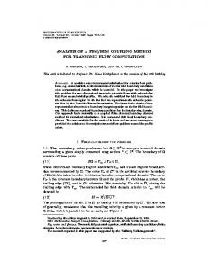
1 Introduction For certain categories of problems, neither the boundary element method (BEM) nor the finite element method (FEM) is best suited and it is natural to attempt to couple these two methods in an effort to create a finite elementboundary element method (FEBEM) that combines all their advantages and reduces their disadvantages. Unfortunately, the systems of equations, produced by the two methods, are expressed in terms of different variables and cannot be linked as they stand. The coupling of the two methods has been a topic of great interest for more than two decades. The conventional coupling methods [1-17] employ an entire unified equation for the whole domain, by combining the discretized equations for the BEM and FEM sub-domains. The algorithm for constructing an entire equation is highly complicated when compared with that for each single equation. In order to overcome the stated inconvenience, iterative domain decomposition coupling approaches were developed [18-24], where there is a no need to combine the coefficient matrix for the FEM and BEM sub-domains. A second advantage is that different formulation of the FEM and BEM can be adopted as base programs for coupling the computer codes only. In these coupling algorithms, separate computing for each subdomain and successive renewal of the variables on the interface of the both sub-domains are performed to reach the final convergence. Gerstle et al. [18] and Perera et al. [19] presented solution schemes, which utilize the conjugate gradient method and the Schur complement, respectively, for the renewal of the unknowns at the interface. Kamiya et al. [20] employed the renewal schemes known as Schwarz Neumann-Neumann and Schwarz Dirichlet-Neumann. Kamiya and Iwase [21] introduced an iterative analysis using conjugate gradient and condensation. Lin et al. [22], and Feng and Owen [23] presented a method which is considered as a sequential form of the Schwarz DirichletNeumann method. Elleithy and Al-Gahtani [24] presented an overlapping iterative domain decomposition method for
coupling of the FEM and BEM. The domain of the original problem is subdivided into a FEM sub-domain, a BEM subdomain, and a common region, which is modeled by both methods. The above iterative coupling methods, however, are only limited to linear problems. The objective of this paper is to extend the application of the sequential Schwarz DirichletNeumann iterative coupling method to elasto-plasticity. Applications in fracture mechanics are considered. The conventional FEM computations are also performed, and a critical comparison of the results is made.
2 Iterative Coupling Method in ElastoPlasticity In this section we consider the extension of the sequential Schwarz Dirichlet-Neumann iterative coupling method presented by Lin et al. [22], and Feng and Owen [23] to elasto-plasticity. As any other coupling procedure, the starting point is to decompose the domain of the original
problem W into two sub-domains W and us define the following vectors (Figure 1): B
{uB }:
{u }: I B
W
F
. Now, let
displacement in the BEM sub-domain, displacement on the BEM/FEM interface (but it is approached from the BEM sub-domain),
{u }: displacement in the BEM sub-domain except B B
{u }, I B
{uF }:
{u }: I F
{u B }= {uBB , uBI }T
displacement in the FEM sub-domain, displacement on the BEM/FEM interface (approached from the FEM sub-domain), and
FEM/BEM Interface G
I
BEM Sub-domain
FEM Sub-domain
Domain of the Original Problem
G
F
G W
{u } {f } F F
F
F F
{u } {u } {t } {f }
{u } {t } B B
I B
W
I B
I F
B
B B
B
I F
{uB }= {uBB , uBI }
{uF }= {uFF , uFI }
T
T
BEM Modeling
FEM Modeling
Figure 1: Domain Decomposition
{u }: F F
displacement in the FEM sub-domain except
{u F }= {uFF , uFI }T
{u },
Similarly, one can denote the BEM traction by t BB and t BI and FEM force vectors by f FF and f FI . Disregarding body forces, the assembled boundary element equations for an elastic region are given by:
È H 11 Í H Î 21
H 12 ˘ Ï u ¸ È G 11 Ì ˝ =Í ˙ H 22 ˚ Ó u ˛ Î G 21 B B I B
G 12 ˘ Ï t ¸ Ì ˝ G 22 ˙˚ Ó t ˛ B B I B
(1) For an elasto-plastic analysis, the incremental form of the FEM equations can be written as:
I F
È K 11 Í K Î 21
Ï D f FF ¸ K 12 ˘ Ï D uFF ¸ = Ì ˝ Ì I ˝ K 22 ˙˚ Ó D uFI ˛ Ó D fF ˛
(2)
It should be noted that for each load increment, Equations (2) are nonlinear and therefore are solved iteratively. At the interface, the compatibility and equilibrium conditions should be satisfied, i.e.,
{u }= {u } ΠG {f }+ [M ]{t }= 0 I B
I F
I F
I
I B
(3)
ΠG
I
(4)
[ ]
where, M is the converting matrix due to the weighing of the boundary tractions by the interpolation functions on the interface. The iterative coupling method can be summarized as follows:
1.
Given the initial guess
2.
For
{u }= {u}.
intensity factor that is only 1.9% different than the analytical solution, while the FEM gives an error of 5.9%. The difference in CPU time recorded for both methods is insignificant and therefore a comparison of the results is not given here.
I B,0
n = 0, 1, 2,........ , do
{t } Solve Equation (4) and obtain {f } I B,n
Solve Equation (1) and get
I F,n
For
i = 1,
3.2. Non-Linear Fracture Mechanics Example
2, ....... , specified number of increments
{D u } u } = {u } + {Äu } Apply { Obtain { u } Apply { u }=(1 - a ){u }+ a {u } I F,i n
Solve Equation (2) for I F,i + 1 n
I F,i n
I F,i n
I F ,n
where Until
a
I B, n+ 1
{u
I B, n
I F, n
is a relaxation parameter
}- {u }