Computational studies in epigenomics using ... - Infoscience - EPFL

Computational studies in epigenomics using histone modification data

THÈSE NO 6327 (2014) PRÉSENTÉE LE 28 AOÛT 2014 À LA FACULTÉ INFORMATIQUE ET COMMUNICATIONS

LABORATOIRE DE BIOLOGIE COMPUTATIONNELLE ET BIOINFORMATIQUE

PROGRAMME DOCTORAL EN INFORMATIQUE, COMMUNICATIONS ET INFORMATION

ÉCOLE POLYTECHNIQUE FÉDÉRALE DE LAUSANNE POUR L'OBTENTION DU GRADE DE DOCTEUR ÈS SCIENCES

PAR

Nishanth Ulhas NAIR

acceptée sur proposition du jury: Prof. E. Telatar, président du jury Prof. B. Moret, Dr Ph. Bucher, directeurs de thèse Prof. S. Hannenhalli, rapporteur Prof. F. Naef, rapporteur Prof. W. Stafford Noble, rapporteur

Suisse 2014

— verse 32 in Sri Guru Gita (authored by sage Vyasa)

To my wonderful mother and father. To my beloved wife. To my teachers, advisors, mentors. To the great Masters, to whom I can but humbly bow.

Acknowledgements To say I have had a very blessed student life would be an understatement. Although as long as one is in the world of academics one is always a student, I understand that with the completion of my PhD, I may not get an other opportunity to be a formal student of science and technology again. There are a countless people who I am deeply indebted to throughout my life without who I would not have such a wonderful student life. I would like to thank all of them and name a few below. First and foremost I would like to thank my PhD advisor Prof. Bernard M.E. Moret for making me a part of the Laboratory of Computational Biology and Bioinformatics (LCBB) lab. Bernard is one of the best advisors anyone can get and I am very lucky to have him as my advisor. I don’t think any advisor gives more freedom to his/her students than Bernard does. Bernard gave me a lot of freedom and at the same time guided me well throughout my PhD with a lot of compassion as well as patience. Many times I found him more as a friend than an advisor and I had many non-technical discussions with him too... especially about politics, governance, and society. I am grateful to Bernard for making me a part of this lab even though I had a non-CS and non-Biology background. In fact Bernard was kind enough to come all the way to India just to attend my wedding ! Thank you Bernard for all that you have done for me. Most students are lucky to have one good advisor... but I had two ! Dr. Philipp Bucher is my other PhD advisor and he has been a truly amazing. He is a person who is full of ideas and every time I met him I learned something new. He has been very patiently and compassionately helping me throughout the duration of my PhD. Thank you Philipp for everything. The Guru-Shishya parampara (teacher-disciple tradition) is well known in India. The word "Gu" means darkness while the word "Ru" means dispeller — dispelling darkness. Guru is thus the one who removes your ignorance. My mother Mrs. Vimala V.N. Pillai — who I call Amma — is my first Guru. Amma’s infinite compassion, her love and dedication towards my well-being and education is primarily responsible for me to complete my PhD. She has almost super-human levels of tolerance towards the most adverse situations and her dedication and sincerity to everyone she meets is a constant source of inspiration for me. She is also one of the most intelligent and insightful people that I know and I constantly look up to her for advice and protection. I don’t think I could have asked for a better mother than her. I feel extremely blessed to be her son. v

Acknowledgements My father Mr. D. Ullas — who I call Achha — has been very loving and compassionate towards me. Achha has got an extraordinary energy and is full of good humour. He has struggled a lot to give me a good education and life and has been very supportive of my career decisions. With immense gratitude I thank Amma and Achhan for all that they have done for me and for being my parents. My brother Nitin has always been my well-wisher. We used to play a lot together when we were kids, and had a lot of fun doing so. He has been constantly supportive of me, and been my well-wisher... and I thank him very much for it. I am also deeply grateful to my grandmother Mrs. Janaky Amma (whom I fondly call Ammooma) for her blessings and love towards me. I would also like to thank my other relatives who have helped and advised me and my family a lot along the way. In particular I would like to express my deep love and affection to my cousins Ashwin Dinesh (fondly called Achhu) and Nandana. Ever since my childhood, when it came to my education, things somehow by magic seemed to work, as if the Universe was aligning itself in a way such that I get a fine education. I was very lucky to get into a great school like St. Joseph’s Boys’ High School in Bangalore. It is one of the oldest and finest schools in the country. My parents struggled a lot and put me into this school although it was beyond their means. A person named Shaji whom I have never met played a role in getting me admission into this school. I thank him for that. Studying at St. Joseph’s Boys’ High School gave me an excellent exposure to the opportunities outside. I had a very good time in the school and learnt a lot from my teachers like Mrs. Sandhya Raman, Mr. Uday Kumar, Dr. David Chatterjee and others. One of my seniors in school, the extremely bright Dr. Sriram Sankararaman has been a constant source of inspiration for me, and it was partly because of him that I chose to pick computational biology as my area of research. I was also very fortunate to study at BASE which is a very fine coaching institute for IIT-JEE exams. Although I did not make it into the IITs, I learnt a lot by going there and my love for physics, organic chemistry, and mathematics developed quite a bit during my time there. The teachers at BASE and the founder of the institute Dr. H.S. Nagaraja (often called HSN) were people of great dedication and sincerity. I would like to thank my B.E. friends — Mushaffa, Manjunath, Karthik, Srinivas for their friendship during my undergraduate days. Probably the finest moment of my academic life came when I got admission into Indian Institute of Science (IISc), Bangalore for my Masters degree. IISc is one of the oldest and probably the finest graduate level research university in India, and I was very lucky to study at the Electrical Communication Engineering department which is one of the best departments at IISc. vi

Acknowledgements I had a great advisor in Prof. T.V. Sreenivas during my study at IISc. TVS sir was not just a great advisor technically, he also taught me a lot about life. We used have wonderful philosophical discussions and I am extremely grateful to him for everything that he has done for me. At IISc, I also had an opportunity to meet some excellent friends and met some amazing people. To name a few, I would like to thank Sreeram, Basavaraj, Sudha, Anoop and his wife Anusha, Dinesh, Arun, Manasa, Nadir, Narayana, Venkat, Saikat, Mrugesh, Sriram etc. to name a few. I am very grateful to Mrugesh for getting me interested in yoga and spirituality by giving me the book “The Power of Now” written by Eckhart Tolle, which is the first book on spirituality that I read. I got an opportunity to work in a wonderful place like Microsoft Research India (MSRI) for a year as soon as I finished my Masters degree at IISc. I would like to thank my advisor Dr. Navin Goyal for his support. I also thank Kalika Bali, Dr. Amitava Das, and Prof. Nagasuma R. Chandra who advised me during my stay there. I also got some good friends — like Cohan, Santhosh, Meena, Sneha. Through my interaction with some of them I also got to meet Lakshmi Dinesh who turned out be an excellent friend over all these years. I remember longing to do a PhD ever since my childhood days and I was extremely delighted to get an admission into a world class institute like EPFL. EPFL is a wonderful place for research and study. I have had a very beautiful time during my stay in Switzerland. I was lucky to be a part of the Laboratory of Computational Biology and Bioinformatics (LCBB), which was an excellent place to be, thanks to Bernard and all my colleagues there. I would like to thank lab mates Avinash, Xiuwei, Wei, Yu, Vaibhav, Mingfu, Cristina, Min, Yann, Krister, Slavica, Olga, Ana, Jelena, Paulina, Laura, Hermina, Aleksandra, Alisa for all their friendship and support. I was lucky to collaborate with some exceptionally bright people during my PhD days, other than my advisors. My collaboration started with Avinash Das Sahu, who is one of the brightest and smartest person that I have met ; and I doubt if my PhD would have happened without his support and immense help. I also had good collaborations with Dr. Yu Lin, Dr. Sunil Kumar, Ana Manasovska, Paulina Grnarova, Jelena Antic, Prof. Judy A Brusslan, Prof. Matteo Pellegrini, Dr. Vaibhav Rajan, Laura Hunter, Mingfu Shao. I thank them all. I had an opportunity to mentor a few extremely bright students — Ana, Paulina, Jelena, and Laura. I thank all of them for giving me this opportunity. In fact I am proud to say that Ana, Paulina, Jelena got their first publication through their collaboration with me. I am grateful to Prof. Sridhar Hannenhalli, Prof. William Stafford Noble, Prof. Emre Telatar, Prof. Felix Naef for being a part of my PhD thesis jury committee. Along with my two advisors Bernard and Philipp, they carefully read my thesis and giving me valuable feedback. I would like to thank them for that. My life in Switzerland would not have been so great if it wasn’t for some amazing friends I had. In specific I would like to thank my best friends Dr. Abhishek Tewari, Avinash Das Sahu, and Dr. Rammohan Narendula who I would like to keep in touch throughout my life. Abhishek vii

Acknowledgements has been my closest friend throughout my PhD days. He had joined at the same time as I did, and he stayed in the opposite door studio in the same building that I lived during most of my PhD days. We cooked together on most days and we had excellent discussions on Indian politics, society, philosophy, spirituality etc. In fact Abhishek, Ram, and I used to take active interest in Indian politics and participate in several ways. My life here would have been boring if not for Abhishek’s genuine friendship and compassion. I am deeply indebted to him for that. Avinash is an incredible person who lives a very interesting life. He is truly brilliant and very good at many things. Other than helping me a lot of research and academic subjects, I also learnt a lot about Indian society and culture, politics and many other things from him. He also helped a lot during any personal difficulty I had. I thank him for that. Ram became my very good friend during my last 2-3 years of PhD. Our “tea with Ram” sessions everyday used to be a delightful time, when many of us would meet for tea in Ram’s lab library and discuss many things — especially Indian politics. Ram was always known for getting amazingly cheap offers and deals. He is an avid traveler, and I traveled a lot with him around Switzerland. I had many other wonderful friends at EPFL. Rajasunder Chandran (Raja) has been a great friend who is deeply passionate about what he does, and he is very sincere, innocent, and compassionate person. I also enjoyed the friendship of Rahul VV who helped me quite a bit. Some of the other friends I would like to thank are Suri, Saket, Vandana, Megha, Pankaj, Rishikesh, Arnab, Aviinash, Krishnan, Devika among many others. I am grateful to Devika for starting the Gita self-study group and it is something I have immensely enjoyed and learnt a lot over the last few years. It was truly amazing that few of us — mainly Devika, Ram, Abhishek, Raja, Giovanni, Krishnan among many others met once a week almost every week for the last two years or so for an hour of Gita class. We studied the Bhagavad Gita Home Study (BGHS) course written by Swami Dayananda Saraswati. So far we finished more than 800 pages of a two-volume book which is around 1800 pages. Giovanni, a Christian priest who I met during the class, has been a great friend. Giovanni is also a scholar on many Indian texts and I learnt a lot from him. He organized some wonderful travels to Florence and Rome, and I learnt a lot from him during these travels. EPFL and Switzerland has offered a lot to me. Other than good education and research facilities, EPFL offers a very good PhD stipend which helped me and my family a lot financially. Coming to Switzerland was very good for me health wise too — I did not suffer from the allergies which I often suffered from in India. I cannot but be awed my the beauty of Switzerland — the gorgeous mountains and lakes. I am equally awed by the countless Swiss engineers and workers who made the roads, tunnels, railways in Switzerland to make these mountains so accessible for us. In fact Amma who is currently in Switzerland visiting me remarked “God and man has strived in equal capacity to make Switzerland what it is” (this is an approximate translation of her remark made in Malayalam). I made some great friends via Facebook like Vinay Vaidya and Dafne (both of whom I have never met), and I learnt a lot from my interactions with them. My dear friend Dr. Sreeram Kannan played a very important role in my life, especially as a spiritual guide. He introduced viii

Acknowledgements me to the “Inner Engineering” program designed by Sadhguru. I thank him very much for everything. During my PhD, I had an opportunity to attend a semester long program “Mathematical and Computational Approaches in High Throughput Genomics,” organized by Institute of Pure and Applied Mathematics (IPAM), University of California, Los Angeles. I would like to thank IPAM for organizing such a great program. I had a great time in Los Angeles, and an opportunity to collaborate with wonderful researchers like Prof. Matteo Pellegrini. I also got some good friends like Dr. Greg Ryslik. I would like to thank my in-laws Mrs. T.V. Meera Nambiar (who I call Mummy), Mr. E.K. Krishnan Nambiar (who I call Daddy) for all their love and support ; and for allowing me to be Asha’s husband. I would also like to thank Asha’s brother Mr. Anu Krishna for all his support and compassion. I am deeply grateful to my lovely wife Dr. Asha Krishna. We had an arranged marriage, and did not really know each other well before the wedding. We got married on January 8th, 2014 ; and the last few months has been among the best in my life. Asha has been the most loving and compassionate wife. I consider myself fortunate to receive her love and affection, and consider myself lucky to be her husband. Thank you muthee for everything. I humbly bow to the great Masters of Yoga to whom I am ever grateful. In India, among all human relationships, the relationship between a Guru (spiritual Master) and Shishya (student/seeker) is considered the highest. Because it is the only relationship which is truly one sided — in that a Guru only gives without expecting anything in return from the student except the student’s growth, while a student only takes without having anything to offer in return. I learnt a lot from studying the teachings of great Masters of Yoga (and Advaita Vendanta or nondualism) like Bhagavan Sri Ramana Maharshi, Sri Nisargadatta Maharaj, Eckhart Tolle, among many others, and by reading some of the commentary of the Sashtras by Swami Dayananda Saraswati. I am deeply grateful to all the ancient Gurus who walked on this planet all the way upto the first Guru or the Adiguru — Adiyogi Shiva — who is worshiped as Dakshinamurthy, the South-facing Jnana aspect of Shiva. I guess I am blessed to be born in India which has an extraordinary spiritual tradition. And I am most grateful to Sadhguru Jaggi Vasudev for being my Master. Sadhguru came into my life when I was looking for a living Master. Finally I thank the Greatest Guru of them all — Life. Lausanne, August 28, 2014

Nishanth Ulhas Nair

ix

Abstract Epigenetic factors like histone modifications are known to play an important role in gene regulation and cell differentiation. Recently, thanks to advances in technologies like ChIP-Seq which is a high-throughput, high resolution, and low cost technology for studying histone modifications and transcription factors, we have large amounts of data available. Therefore computational techniques become important for studying and interpreting this data. In this thesis, we have focused on primarily building computational methods to analyze and study ChIP-Seq histone modification data. The work can be divided into two broad topics : (a) to process ChIP-Seq data computationally and to identify regions of biological interest ; (b) to use processed data for higher-level analysis to study problems in cell differentiation and evolution of cell types, based on phylogenetic approaches. In the first topic, this thesis makes a contribution by addressing two problems : (i) We propose a two-stage statistical method, called ChIPnorm, to normalize ChIP-Seq data, and to find differential regions in the genome, given two libraries of histone modifications of different cell types. We show that our method removes most of the bias in the data and also provides a normalization that enables direct comparison of values between the two cell types. We show that our method outperforms the state of the art techniques in literature. (ii) We propose probabilistic partitioning methods to discover significant patterns in ChIP-Seq data. Our methods work on the principle of expectation-maximization, is simple and flexible, and takes into account signal magnitude, shape, strand orientation, and shifts. It runs in linear time and gives improved results on the state of the art techniques especially when used on sparse data. In the second topic, we try to provide a link between the fields of epigenomics and evolution. We introduce the concept of cell-type trees based on the principles of phylogenetic inference on ChIP-Seq histone modification data. These cell-type trees are precisely defined and algorithmic techniques are designed to infer these trees from the data. In the process, we develop new data representation techniques and also a peak-finder to help us build good cell-type trees. We obtain biologically meaningful results and show that cell-type trees have the potential to study cell differentiation and the evolution of cell types across species. Key words : epigenomics, epigenetics, histone modifications, ChIP-Seq, cell-type trees, evolution, phylogeny, evolution of cell types, ChIPnorm, probabilistic partitioning, expectation maximization, phylogenetic trees.

xi

Résumé Les facteurs épigénétiques, tels que les modifications des histones, joueent un rôle important dans la régulation des gènes et la différenciation cellulaire. Le développement récent de la technologie ChIP-Seq, une méthode de laboratoire de haut débit, haute précision, et faible coût, a mis à disposition des chercheurs de grandes quantité de données pour létude des modifications de l’histone et des facteurs de transcription. Le développment de techniques de calcul pour analyser ces données prend donc une place importante dans la recherche. Dans cette thèse, nous présentons de telles techniques de calcul pour l’analyse des données ChIP-Seq sur la modification des histones. Le travail couvre deux thèmes principaux : (a) les méthodes requises pour traiter les données brutes de ChIP-Seq et d’y identifier les régions d’intérêt dans les sciences de la vie ; et (b) des méthodes pour analyser ces régions à plus haut niveau pour approfondir nos connaissances dans le domaine de la différenciation cellulaire et l’évolution des types de cellules. Sous le premier thème, cette thèse contribue des solutions à deux problèmes. La première est une méthode statistique en deux étapes, ChIPnorm, pour normaliser les données de ChIP-Seq et s’en servir pour déceler des régions différentielles dans le génome, étant données deux bibliothèques de modifications des histones de différents types cellulaires. Notre méthode supprime la plupart des biais dans les données et permet une comparaison directe des valeurs entre les deux types cellulaires ; nous montrons qu’elle surpasse l’état de l’art dans ce domaine. La deuxième est une méthode de partitionnement probabiliste pour découvrir des modèles intèressants dans les données de ChIP-Seq. Notre méthode fonctionne sur le principe de l’espérance-maximisation, est simple et flexible, et prend en compte l’amplitude and la forme du signal, l’orientation des chaînes, et le déphasage. Il tourne en temps linéaire et surpasse l’état de l’art, en particulier pour les données éparses. Sous le second thème, nous étudions les liens entre l’épigenomique et l’évolution. Nous introduisons le concept d’arbres cellulaires, construits selon les principes de l’inférence phylogénétique sur la base de données de modification des histones. Nous donnons une définition précise de ces arbres aussi bien que des algorithmes pour les construire à partir des données ChIP-Seq. Ces algorithmes utilisent de nouvelles représentations de ces données et un nouveau moteur de recherche pour les pics. Nous obtenons des résultats biologiquement pertinents et démontrons que les arbres cellulaires offrent un outil valable dans l’étude de la différenciation cellulaire et de l’évolution des types de cellules. xiii

Acknowledgements Mots clefs : l’épigénétique, les modifications des histones, ChIP-Seq, arbres cellulaires, évolution, phylogénie, évolution des types de cellules, ChIPnorm, partitionnement probabiliste, espérancemaximisation

xiv

Contents Acknowledgements

v

Abstract (English/Français)

xi

List of figures

xvii

List of tables

xxiii

1 Introduction 2 Background 2.1 Biological concepts . . . . . . . . . . . . . . . . 2.1.1 Epigenetics and Histone Modifications 2.1.2 Phylogenetic trees . . . . . . . . . . . . 2.1.3 Developmental biology and Evolution 2.2 Experimental technology and data . . . . . . . 2.2.1 ChIP-Seq technology . . . . . . . . . . . 2.2.2 Common data formats . . . . . . . . . . 2.2.3 Data availability . . . . . . . . . . . . . . 2.2.4 Data visualization . . . . . . . . . . . . . 2.3 Computational Methods . . . . . . . . . . . . . 2.3.1 Data representation . . . . . . . . . . . 2.3.2 Statistical measures . . . . . . . . . . . 2.3.3 Normalization techniques . . . . . . . . 2.3.4 Expectation-maximization algorithm . 2.3.5 Phylogenetic tree building methods . . 2.3.6 Minimum spanning tree . . . . . . . . .

1

. . . . . . . . . . . . . . . .

. . . . . . . . . . . . . . . .

. . . . . . . . . . . . . . . .

. . . . . . . . . . . . . . . .

. . . . . . . . . . . . . . . .

. . . . . . . . . . . . . . . .

. . . . . . . . . . . . . . . .

. . . . . . . . . . . . . . . .

. . . . . . . . . . . . . . . .

. . . . . . . . . . . . . . . .

. . . . . . . . . . . . . . . .

. . . . . . . . . . . . . . . .

. . . . . . . . . . . . . . . .

. . . . . . . . . . . . . . . .

. . . . . . . . . . . . . . . .

. . . . . . . . . . . . . . . .

. . . . . . . . . . . . . . . .

. . . . . . . . . . . . . . . .

. . . . . . . . . . . . . . . .

. . . . . . . . . . . . . . . .

3 ChIPnorm: a statistical method for normalizing and identifying differential regions in histone modification ChIP-Seq libraries 3.1 Introduction . . . . . . . . . . . . . . . . . . . . . . . . . . . . . . . . . . . . . . . . 3.2 Methods . . . . . . . . . . . . . . . . . . . . . . . . . . . . . . . . . . . . . . . . . . 3.2.1 ChIPnorm scheme . . . . . . . . . . . . . . . . . . . . . . . . . . . . . . . . 3.2.2 Stochastic noise ε . . . . . . . . . . . . . . . . . . . . . . . . . . . . . . . . . 3.2.3 Local genomic bias ν . . . . . . . . . . . . . . . . . . . . . . . . . . . . . . .

5 5 5 6 6 8 8 9 10 10 10 10 12 13 13 14 15

17 17 19 21 21 23 xv

Contents 3.2.4 Quantile normalization . . . . . . . . . . . . . . . . . . . . . . . . . . . . .

24

3.2.5 The complete ChIPnorm method summarized . . . . . . . . . . . . . . .

27

3.3 Experimental Design . . . . . . . . . . . . . . . . . . . . . . . . . . . . . . . . . . .

28

3.4 Results . . . . . . . . . . . . . . . . . . . . . . . . . . . . . . . . . . . . . . . . . . .

29

3.4.1 Comparative Analysis . . . . . . . . . . . . . . . . . . . . . . . . . . . . . .

30

3.4.2 Correlation with gene expression . . . . . . . . . . . . . . . . . . . . . . . .

37

3.4.3 Bivalent region analysis . . . . . . . . . . . . . . . . . . . . . . . . . . . . .

38

3.4.4 Differential enriched regions along protein-coding genes . . . . . . . . .

40

3.4.5 Using ChIPnorm in analyzing histone modification data from Arabidopsis 40 3.4.6 Software Availability . . . . . . . . . . . . . . . . . . . . . . . . . . . . . . .

42

3.5 Conclusion . . . . . . . . . . . . . . . . . . . . . . . . . . . . . . . . . . . . . . . . .

42

4 Probabilistic partitioning methods to find significant patterns in ChIP-Seq data 4.1 Introduction . . . . . . . . . . . . . . . . . . . . . . . . . . . . . . . . . . . . . . . .

43

4.2 Methods . . . . . . . . . . . . . . . . . . . . . . . . . . . . . . . . . . . . . . . . . .

46

4.2.1 Expectation-Maximization (EM) algorithm . . . . . . . . . . . . . . . . . .

46

4.2.2 Modified “Shape-Only” EM algorithm . . . . . . . . . . . . . . . . . . . . .

46

4.2.3 Variations - with shift and flip . . . . . . . . . . . . . . . . . . . . . . . . . .

47

4.2.4 Seeding and initialization strategies . . . . . . . . . . . . . . . . . . . . . .

48

4.3 Results and Discussion . . . . . . . . . . . . . . . . . . . . . . . . . . . . . . . . . .

49

4.3.1 On simulated data . . . . . . . . . . . . . . . . . . . . . . . . . . . . . . . .

49

4.3.2 On real ChIP-Seq data . . . . . . . . . . . . . . . . . . . . . . . . . . . . . .

53

4.4 Conclusion . . . . . . . . . . . . . . . . . . . . . . . . . . . . . . . . . . . . . . . . .

62

5 Cell-type trees 5.1 Introduction . . . . . . . . . . . . . . . . . . . . . . . . . . . . . . . . . . . . . . . .

63 63

5.2 Methods . . . . . . . . . . . . . . . . . . . . . . . . . . . . . . . . . . . . . . . . . .

65

5.2.1 Model of differentiation for histone marks . . . . . . . . . . . . . . . . . .

65

5.2.2 Data representation techniques . . . . . . . . . . . . . . . . . . . . . . . .

65

5.2.3 Phylogenetic analysis . . . . . . . . . . . . . . . . . . . . . . . . . . . . . .

67

5.2.4 On the inference of ancestral nodes . . . . . . . . . . . . . . . . . . . . . .

68

5.2.5 Peak-finding . . . . . . . . . . . . . . . . . . . . . . . . . . . . . . . . . . . .

68

5.3 Results and Discussion . . . . . . . . . . . . . . . . . . . . . . . . . . . . . . . . . .

69

5.3.1 Code . . . . . . . . . . . . . . . . . . . . . . . . . . . . . . . . . . . . . . . .

85

5.4 Conclusions . . . . . . . . . . . . . . . . . . . . . . . . . . . . . . . . . . . . . . . .

85

6 Further study using cell-type trees 6.1 Introduction . . . . . . . . . . . . . . . . . . . . . . . . . . . . . . . . . . . . . . . .

xvi

43

87 87

6.2 Lifting: inferring ancestral nodes . . . . . . . . . . . . . . . . . . . . . . . . . . . .

87

6.2.1 Algorithm for lifting . . . . . . . . . . . . . . . . . . . . . . . . . . . . . . .

87

6.2.2 Results and Discussion . . . . . . . . . . . . . . . . . . . . . . . . . . . . . .

88

6.3 Using normalized raw data . . . . . . . . . . . . . . . . . . . . . . . . . . . . . . .

91

6.3.1 Evaluation of different data representations . . . . . . . . . . . . . . . . .

91

Contents 6.4 Comparing human and mouse cell types . . . . . . . . . . . . . . . . . . . . . . . 6.5 Conclusion . . . . . . . . . . . . . . . . . . . . . . . . . . . . . . . . . . . . . . . . . 7 Conclusions A Appendix for Chapter 4 A.1 R code for probabilistic partitioning . . . . . . . . . . . . . . . . . . . . . . . . . A.1.1 Expectation-Maximization step for basic ChIP-partitioning algorithm . A.1.2 Complete algorithm for partitioning with random seeds . . . . . . . . . A.1.3 Iterative partitioning - standard version for two classes . . . . . . . . . A.1.4 Iterative EM partitioning with untrained flat class . . . . . . . . . . . . . A.1.5 Variations of the EM algorithm - shape-based partitioning . . . . . . . A.1.6 Shape-based partitioning with flips . . . . . . . . . . . . . . . . . . . . . A.1.7 Shape-based partitioning with shifts . . . . . . . . . . . . . . . . . . . . A.1.8 Shape-based partitioning with flips and shifts . . . . . . . . . . . . . . . A.2 R code for generating simulated data . . . . . . . . . . . . . . . . . . . . . . . . A.2.1 Two classes without shifts and flips . . . . . . . . . . . . . . . . . . . . . A.2.2 Two classes with flips . . . . . . . . . . . . . . . . . . . . . . . . . . . . . . A.2.3 Four classes . . . . . . . . . . . . . . . . . . . . . . . . . . . . . . . . . . . A.2.4 Two classes characterized by co-localizing peaks of different width . .

93 94 97

. . . . . . . . . . . . . .

99 99 99 100 100 101 101 102 102 103 104 104 104 105 106

B Appendix for Chapter 5

107

Bibliography

121

Curriculum Vitae

123

xvii

List of Figures

2.1 Example of a phylogenetic tree (source: http://sites.duke.edu/dukeresearch/2011/11/14/being-the-shy-kid-may-have-its-ben and adapted from http://phylogenous.files.wordpress.com/2011/01/treea.png). . . . . . . . . 6 2.2 Example of cell-differentiation among blood cells (source: Wikipedia). The arrows indicate a tree structure. . . . . . . . . . . . . . . . . . . . . . . . . . . . . . . . . . . . . . . . . . . .

7

2.3 The various steps in the ChIP-Seq procedure are shown (source Wikipedia). . . . . . . . . . . .

9

2.4 Profile of a ChIP-Seq data library. Signal above some threshold are classified as peaks. . . . . . .

11

2.5 Profile of two ChIP-Seq data libraries L1 and L2. Differential regions in the genome are marked. .

11

3.1 Histone modification profile as seen in the UCSC genome browser [61]. Tracks 1 (red) and 2 (green) show the H3K27me3 modifications for ES and NP cells, respectively. Track 3 shows the differentially enriched regions found by our ChIPnorm method. Track 4 shows the differentially enriched regions found by the ChIPDiff method [125]. In tracks 3 and 4, red indicates differential enrichment in ES

. . .

20

3.2 Overview of ChIP-Seq process. We see how we can get the ChIP-Seq library, input DNA control, and the random distribution (null hypothesis). . . . . . . . . . . . . . . . . . . . . . . . . . . .

22

cells and green indicates differential enrichment in NP cells. Track 5 shows the UCSC genes.

3.3 An example of random distribution (amplified binomial distribution with α = 2) is shown in red and the estimated real distribution of the original ChIP-Seq data for one chromosome is also shown (blue). ABD — amplified binomial distribution. Data probability — estimated real distribution.

. . . . . . . . . . . . . . . . . . . . . . .

23

3.4 Iterative Normalization of input DNA. (a) before first iteration. (b) after first iteration, post removal of outliers. . . . . . . . . . . . . . . . . . . . . . . . . . . . . . . . . . . . . . . . . . .

24

3.5 The new inverse cumulative distribution function on the modified libraries (after stage 1). On the x axis is the percentile, on the y axis are the bin values. . . . . . . . . . . . . . . . . . . . . . .

26

The figure is zoomed into a small region for clarity.

3.6 The schematic diagram of the ChIPnorm method. In the first stage one we find the enrichedsignificant bins by removing various kinds of errors in the data. In the second stage we normalize the two ChIP-Seq libraries and find differentially enriched bins.

. . . . . . . . . . . . . . . . .

27

3.7 Enrichment level of bins with respect to gene density in a 1 Mbp region. The x axis indicates lowest to highest gene density. (a) The y axis indicates the total number of H3K27me3 ChIP-Seq fragments divided by the number of Mbp regions (counts per megabase) found in each gene density. (b) The plots are re-normalized so that the y axis range is same for both ES and NP cell data. We see that the enrichment level of ChIP-Seq data increases with respect to gene density for both ES and NP cells.

31 xix

List of Figures 3.8 Enriched bins with respect to gene density in 1 Mbp region. The plots are normalized. x axis 1 to 10 indicates lowest to highest gene density, while y axis 0 to 1 indicates minimum to maximum average number of differentially enriched bins for both ES and NP cells. Blue line indicates ES differentially enriched bins and red line indicates NP differentially enriched bins. The number of enriched bins per 1 Mbp should increase with gene density.

3.9 Plot of

. . . . . . . . . . . . . . . . . . .

32

sensitivity (sensitivity + error) over five different threshold values. (a) NP is differentially over-expressed

compared to ES, (b) ES is differentially over-expressed compared to NP.

. . . . . . . . . . . . .

34

3.10 Robustness studies: sensitivity and error analysis for ChIPnorm by fixing the fold-change threshold τ = 3 and varying the bin size from 200 bp to 2000 bp in steps of 200 bp. Data from Mikkelsen et al. 2007 [85].

. . . . . . . . . . . . . . . . . . . . . . . . . . . . . . . . . . . . . . . . . . .

35

3.11 Two ROC curves are shown for various methods. (a) first ROC: Class 1 - four-fold NP differentially over-expressed genes compared to ES; Class 0: rest of the genes. (b) second ROC: Class 1 - four-fold ES differentially over-expressed genes compared to NP; Class 0: rest of the genes.

. . . . . . . . .

37

3.12 Gene profile according to expression and histone modifications. Genes are grouped in (A-E) according to increasing ratio of expression level in ES cells and NP cells. Within each groups, genes are classified into 4 types. Type 2 genes have differential histone enrichment in ES cells in their promoter regions and type 4 genes have differential enrichment in NP cells. (a) Percentage of type 2 genes is decreasing, while percentage of type 4 genes is increasing along the group (A-E). (b) Percentage of type 2 genes is increasing, while percentage of type 4 genes is decreasing along the group (A-E).

. .

38

3.13 Bivalent regions in genes: in 333 selected genes and in UCSC known genes. Genes are attributed to classes according to the presence of modifications in ES and NP cells. The “A-B” notation in the labels indicates the presence of modification of type “A” in ES cells and modification of type “B” in NP cells. (*) marked labels have bivalent domains in ES cells.

. . . . . . . . . . . . . . . . . .

39

3.14 Bivalent gene profile vs. expression data. Genes are grouped in (A-E) according to increasing ratio of expression level in ES cells and NP cells. Each bar shows the percentage of genes with the corresponding “A-B” modifications (as listed in the box), “A” for modifications in ES cells and “B” for modifications in NP cells. It is seen that there is a strong over-representation of the K4+K27-K4 transition (yellow) in the genes class, which is strongly up-regulated in NP cells.

. . . . . . . . .

40

3.15 Feature aggregate plot of the differential/non-differential regions identified by the ChIPnorm method. Each row corresponds to a region from ChIPnorm and each column corresponds to a genomic feature of protein coding GENCODE genes. Curve inside a cell represents the relative frequency of overlap between the ChIPnorm identified regions and the genomic feature of GENCODE genes, when compared to a similar relative frequency of overlap that would occur by random chance. Figure created using Segtools [18].

. . . . . . . . . . . . . . . . . . . . . . . . . . .

41

4.1 Simulated data without shifts or flips. Shows the data and the patterns found using the the KMeans clustering method, CAGT methods, and the probabilistic partition method (shape-based without shift or flips). Sub-figures a1, b1, c1, d 1, and e1 are for f = 50 and a2, b2, c2, d 2, and e2 are for f = 1. Red is class 1 (class c1 in Table 4.1) and cyan is class 2 (class c2 in Table 4.1).

xx

. . . .

50

List of Figures 4.2 Simulated data with flips. Data (4000 samples) consist of two classes characterized by Gaussianshaped patterns. Each class is represented by two subsets of 1000 samples, one showing the underlying pattern in native, the other one in reversed (flipped) orientation. Sub-figures a1, b1, c1, and d 1 are for f = 50 and a2, b2, c2, and d 2 are for f = 1. b1 and b2 are aggregation plots of the same data but with all samples presented in their native orientation. It can be seen that the probabilistic partitioning method (shape-based) using flips captures the actual data patterns at high ( f = 50) and low ( f = 1) coverage. The CAGT (correlation) method works well for f = 50 only. Red and cyan colors correspond to classes c1 and c2 in Table 4.3, respectively.

. . . . . . . . . . . . . . . . .

53

4.3 Results from experiment with four classes. (a)-(e) Aggregation plots (APs) for simulated data. (f)-(i) Probability weighted APs of samples as classified by the probabilistic partitioning algorithm.

54

4.4 Experiment with two classes characterized by co-localizing Gaussian peaks. Shown are aggregation plots (APs) for the two classes in the data, and for the rediscovered classes obtained with different clustering algorithms. Note that CAGT (correlation) reports only one class. The absence of a second class is reflected by the horizontal red dashed line at height zero in subfigure (c).

. . . .

55

4.5 H3K4me1 and H3K4me3 histone modification data. H3K4me1 and H3K4me3 data mixed together and separated using the K-means, CAGT (correlation), CAGT (Euclidean), and probabilistic partitioning approach (non-shape and shape-based). Red is for the class which represents H3K4me1 and cyan is for H3K4me3 for figures (b) to (h). In the figures, each class is normalized so that the maximum value is 1 for the sake of clarity for each class. Only for sub-figure (b) we normalize using a global maximum of H3K4me1 and H3K4me3.

. . . . . . . . . . . . . . . . . . . . . . . .

56

4.6 Partitioning of nucleosome positioning patterns in human promoters. All curves are drawn to the same scale. Probabilistic partitioning reveals strong oscillatory patterns for subclasses of promoters which partially cancel each other out when mixed together.

. . . . . . . . . . . . .

57

4.7 Aggregation plots (APs) for various genomic features in different promoter classes. (a) APs for different features superposed for the same class. (b) Same feature for different classes in one plot. Position zero corresponds to the transcription start site.

. . . . . . . . . . . . . . . . . . . .

58

4.8 Shape-based peak evaluation with shifting. The figure illustrates the effects of probabilistic partitioning on a CTCF peak list provided by ENCODE in terms of motif enrichment. (a) Probabilistic partitioning with shifting. (b) Partitioning based on original p-values. Method details: CTCF binding motifs where identified by scanning the DNA sequence around peak centers with the JASPAR matrix MA0139.1 at a P-value threshold of 10−5 . The percentage of sequences containing a CTCF motif is plotted in a sliding window of 50 bp. The numbers in parentheses indicate the sizes of the peak lists. For fair comparison, the threshold for partitioning with the original P-values was chosen such as to match the numbers of good and bad peak obtained with probabilistic partitioning. The

. . .

60

4.9 Motif enrichment profiles for IDR-selected ChIP-Seq peak lists. Peak sets were selected at an IDR of 1%. . . . . . . . . . . . . . . . . . . . . . . . . . . . . . . . . . . . . . . . . . . . . .

61

motif enrichment profile for the complete peak list (dotted line) is included in both graphs.

5.1 An example of an interesting region as defined by overlap representation is shown. The dotted horizontal lines represents a portion of the genome. Each row stands for a separate ChIP-Seq library (L1-L5). The dark lines represent peak regions. 1 and 0 is the data representation for each library. .

67 xxi

List of Figures 5.2 ChIPnormSig method to identify significant regions (which are used as peak regions) from histone modification ChIP-Seq library. . . . . . . . . . . . . . . . . . . . . . . . . . . . . . . . . .

69

5.3 Cell-type tree on H3K4me3 data (ENCODE peaks) using only one replicate: (a) windowing representation, (b) overlap representation. . . . . . . . . . . . . . . . . . . . . . . . . . . . . . . .

71

5.4 Using maximum parsimony (TNT software) on H3K4me3 data (ENCODE peaks) using only one replicate (overlap representation). . . . . . . . . . . . . . . . . . . . . . . . . . . . . . . .

73

5.5 Cell-type tree on H3K4me3 data (ENCODE peaks, using all replicates): (a) windowing representation, (b) overlap representation. . . . . . . . . . . . . . . . . . . . . . . . . . . . . . . . .

74

5.6 Cell-type tree on H3K27me3 data (ENCODE peaks), using all replicates and overlap representation. 74 5.7 Cell-type tree using windowing representation on H3K4me1 data. . . . . . . . . . . . . . . . .

75

5.8 Cell-type tree using windowing representation on H3K9me3 data. . . . . . . . . . . . . . . . .

75

5.9 Cell-type tree using windowing representation on H3K27ac data. . . . . . . . . . . . . . . . .

76

5.10 Cell-type tree on H3K4me3 data (ENCODE peaks, using all replicates) on peaks with negative log p-value ≥ 10: (a) windowing representation, (b) overlap representation. . . . . . . . . . . . . .

77

5.11 Overlap representation using overlapping peaks (between replicates) which have an IDR value ≤ 0.025 (output of IDR program). Since the distance between replicates is 0, the two replicates of

. . . . . . . . . . . . . . . . . . . . . . . . . . .

78

5.12 H3K4me3 data (ENCODE peaks), overlap representation on peaks with negative log p-value ≥ 10. Replicate leaves are removed and replaced by their parent. . . . . . . . . . . . . . . . . . . .

79

5.13 Cell-type tree on H3K4me3 data (using one replicate) using (a) windowing representation (b) overlap representation. Peaks generated by ChIPnormSig method (FDR 5%). . . . . . . . . . . . . . .

80

5.14 Cell-type tree on H3K4me3 data (using all replicates) using (a) windowing representation (b) overlap representation. Peaks generated by ChIPnormSig method (FDR 5%). . . . . . . . . . . . . . .

80

5.15 Cell-type tree on H3K4me3 data (using profile data representation) using Overlap representation: (a) ENCODE peaks, (b) ChIPnormSig peaks. . . . . . . . . . . . . . . . . . . . . . . . . . .

81

5.16 Cell-type trees to study evolution of cell types - a constructed example is shown in this figure. Tree T 2 - current species S2. Tree T 1 - ancestral species S1. ST - sub-tree. . . . . . . . . . . . . . .

84

each cell type are represented in one label.

6.1 Part of lifting procedure. An example showing a small portion of the lifting algorithm is shown. The edge between node A and node 2 is the smallest among the considered edges. Therefore node A is lifted upwards to its ancestor and it is made the new leaf.

. . . . . . . . . . . . . . . . . . .

88

6.2 Lifting procedure for ancestral node reconstruction. Shows cell-type tree for H3K4me3 data using overlap representation. The internal nodes are labelled using green edges to one of the cell-types in

. . . . . . . . . . . . . . . . . . . . . . . . . . . . . .

89

6.3 Lifting procedure for ancestral node reconstruction. Shows cell-type tree for H3K4me3 data using overlap representation after lifting process. (Figure is not drawn to scale.) . . . . . . . . . . . .

90

6.4 Minimum spanning tree. Minimum spanning tree for H3K4me3 data using overlap representation (the edges are not drawn to scale). . . . . . . . . . . . . . . . . . . . . . . . . . . . . . . .

91

the leaf node (by lifting procedure).

6.5 Cell-type tree using windowing representation. Data representation using: (a) Peak data, (b) Raw data, (c) Mean normalization of raw data, (d) Mean normalization of raw data (for each chromosome), (e) Standard score normalization of raw data (for each chromosome).

xxii

. . . . . .

95

List of Figures 6.6 Human and mouse cell types. Cell-type tree using overlap representation on human and mouse cell types. Peak data considered only on orthologous regions of human and mouse. . . . . . . . 6.7 Human and mouse cell types by removing some peaks. The number of peaks available for mouse

96

where much more than for human. Therefore the number of peaks used in mouse data were reduced so as to reduce the bias in the results. (Peak data considered only on orthologous regions of human and mouse.) (a) Deleting peaks in mouse data whose negative log p-value is smaller than 50. (b) Divide the genome into windows of 1 Mbp. Then remove those windows if the length of the peak region in either human or mouse data was 50% more than the other (comparing hESC T0 and mE14).

96

B.1 For H3K4me3 data: gene enrichment analysis containing regions of the genome where ES cells (10 replicates) are all 1 and rest of the cell types (62 replicates) have all 0 (one error allowed at most on both sides) using all replicate ENCODE peak data.

. . . . . . . . . . . . . . . . . . . . . . . 108

B.2 For H3K4me3 data: gene enrichment analysis containing regions of the genome where ES cells (10 replicates) are all 0 and rest of the cell types (62 replicates) have all 1 (one error allowed at most on both sides) using all replicate ENCODE peak data.

. . . . . . . . . . . . . . . . . . . . . . . 109

B.3 For H3K27me3 data: gene enrichment analysis containing regions of the genome where ES cells (10 replicates) are all 1 and rest of the cell types (13 replicates) have all 0 (one error allowed at most on both sides) using all replicate ENCODE peak data.

. . . . . . . . . . . . . . . . . . . . . . . 110

B.4 For H3K4me3 data: gene enrichment analysis containing regions of the genome where ES cells for day 0, 2, 5, 9, 14 have a pattern 01000. ENCODE peaks are used and only regions which have identical values of all the replicates for each cell type are considered.

. . . . . . . . . . . . . . 111

B.5 For H3K27me3 data: gene enrichment analysis containing regions of the genome where ES cells for day 0, 2, 5, 9, 14 have a pattern 01000. ENCODE peaks are used and only regions which have identical values of all the replicates for each cell type are considered.

. . . . . . . . . . . . . . 112

xxiii

List of Tables 3.1 Sensitivity analysis percentages using various methods (data from Mikkelsen et al. 2007 [85]). Experiments: unit-mean; quantile; MACS peak finder; ChIPDiff; Rank normalization; two-stage unit-mean; ChIPnorm. The parameters of all the methods (except for MACS as explained in the text) were adjusted so that all of them give almost the same percentage (≈ 15%) of experiment “sensitivity (ES K27-enriched)”.

. . . . . . . . . . . . . . . . . . . . . . . . . . . . . . . . . . . . . .

33

3.2 Values of the various thresholds (T1, T2, T3, T4, T5) used for the various methods used in Figure 3.9. 34 3.3 Sensitivity analysis for human ES and GM12878 cells (replicate 1 data from ENCODE Broad database) percentages using various methods. Experiments: unit-mean; quantile; MACS peak finder; ChIPDiff; Rank normalization; two-stage unit-mean; ChIPnorm. The parameters of all the methods (except for rank normalization as explained in the text) were adjusted so that all of them give almost the same percentage (≈ 11%) of experiment “sensitivity (HES K27-enriched)”.

. . . .

35

3.4 False-positive rate (FPR) analysis for human ES cells (H3K27me3 data from ENCODE Broad database) for the two replicates. We see the percentage of false positive using various methods. Experiments: unit-mean; quantile; MACS peak finder; ChIPDiff; Rank normalization; two-stage unit-mean; ChIPnorm. The thresholds used are same as those in Table 3.3.

. . . . . . . . . . .

37

4.1 Results for simulated data without shifts or flips. Model accuracy is expressed as Pearson correlation coefficient between original and rediscovered patterns/classes. The percentage of samples attributed to a class is shown in parentheses. The classes c1 and c2 correspond to the red and cyan curves in

. . . . . . . . . . . . . . . . . . . . . . . . . . . . . . . . . . . .

51

4.2 Classification error (in percentage) between the discovered patterns and their data classes. . . . .

51

Figure 4.1, respectively.

4.3 Results for simulated data with flips. Model accuracy is expressed as Pearson correlation coefficient between the original and rediscovered patterns/classes. The percentage of samples attributed to a class is shown in parentheses. The classes c1 and c2 correspond to the red and cyan curves in Figure 4.2, respectively.

. . . . . . . . . . . . . . . . . . . . . . . . . . . . . . . . . . . . . . .

52

4.4 Model accuracy (represented by Pearson correlation) and classification error between the discovered patterns and their data classes for the various methods. The time (in seconds) taken for each of the methods is also shown. Real data for H3K4me1 and H3K4me3 around TSS regions are mixed (34741 samples in each dataset with each sample containing 99 bins). The percentage of each class is shown in brackets. H3K4me1 and H3K4me3 stand for the 2 datasets. (Values are rounded to the fourth decimal place for model accuracy and two decimal places for classification error.)

. . . . .

54 xxv

List of Tables 5.1 Cell types, short description, and general group for H3K4me3, H3K27me3, H3K4me1, H3K9me3, H3K27ac data. For details see the ENCODE website [101]. The mark Xshows the usage of that cell type for that particular histone mark.

. . . . . . . . . . . . . . . . . . . . . . . . . . . . .

71

5.2 Statistics for cell-type trees on H3K4me3 data. 2nd to 9th columns show the number of cells (of the same type) belonging to the largest and second-largest clades; the total number of cells of that type is in the top row. Rows correspond to various methods (WM: windowing; OM: overlap; TP: top peaks with threshold of 10). The second last column shows the SR ratio. The last column contains the percent deviation (P D) of the distances between the leaves found using the NJ tree from the Hamming distance between the leaves. ENCODE means peaks from ENCODE data is used while ChIPnormSig means peaks from ChIPnormSig program is used. (one replicate) means only one replicate for each cell type is used, (all replicates) means all available replicates (1, 2, or 3) for each cell type is used, (profile) means a profile representation created using all replicates for each cell type is used. MP - maximum parsimony using TNT software.

. . . . . . . . . . . . . . . . . .

72

5.3 Statistics for cell-type trees on H3K4me3 data using top peaks. 2nd to 9th columns show the number of cells (of the same type) belonging to the largest and second-largest clades; the total number of cells of that type is in the top row. Rows correspond to various methods (OM: overlap; TP: top peaks). threshold x means that the peaks which have a (negative) log p-value ≥ x is used. The second last column shows the SR ratio. The last column contains the percent deviation (P D) of the distances between the leaves found using the neighbor-joining (NJ) tree from the Hamming distance between the leaves. ENCODE peak data is used. (all replicates) means all available replicates (1, 2, or 3) for each cell type is used. We can see that the method is robust to various kinds of threshold used.

77

5.4 Statistics for cell-type trees on H3K4me3 data using IDR analysis. 2nd to 9th columns show the number of cells (of the same type) belonging to the largest and second-largest clades; the total number of cells of that type is in the top row. The second last column shows the SR ratio. The last column contains the percent deviation (P D) of the distances between the leaves found using the NJ tree from the Hamming distance between the leaves. Rows correspond to various methods OM (two replicates): overlap representation on all cell-types which have exactly two replicates (on all available peaks). OM-IDR (two replicates), (threshold x): Overlap representation used on overlapping peaks (between replicates) which have an IDR value ≤ x (output of IDR program). Since these are overlapping peaks the SR ratio is always 0 given the nature of overlap representation. ENCODE peak data is used. (two replicates) means all two replicates for each cell type is used (34 cell-types, 68 libraries). We considered data containing only two replicates for this work.

. . . . .

78

5.5 Analysis on paths. Table shows the number of different types of changes across various days of ES cells. Dx means day x of ES cell type. 1 and 0 represents the presence or absence of a peak as defined by the overlap representation in one region of the genome. The number of such 1-0 patterns are counted and presented in the last column.

. . . . . . . . . . . . . . . . . . . . . . . . . . .

83

5.6 Analysis on paths. Table shows the number of different types of changes for ES, HUVEC, and HBMEC cell types. 1 and 0 represents the presence or absence of a peak as defined by the overlap representation in one region of the genome. The number of such 1-0 patterns are counted and presented in the last column. NA - not applicable (because data for the cell-type is not available).

xxvi

84

List of Tables 5.7 Analysis on paths. Table shows the number of different types of changes for ES, WI38, AG04550, HPF cell types. 1 and 0 represents the presence or absence of a peak as defined by the overlap representation in one region of the genome. The number of such 1-0 patterns are counted and presented in the last column. NA - not applicable (because data for the cell-type is not available).

85

6.1 R ratio. The R ratios for different kinds of data representation are shown for 37 cell-types of H3K4me3 data, each cell-type compared with every other. The frequency of occurrence with a small range of R ratio is shown for all the data representations.

. . . . . . . . . . . . . . . . . . . .

92

6.2 Statistics for cell-type trees on H3K4me3 data for different data representation. 2nd to 9th columns show the number of cells (of the same type) belonging to the largest and second-largest clades (fraction values indicate only one of the two replicates fall in that clade); the total number of cells of that type is in the top row. Fractions are used when only one of the two replicates fall into the clades. Rows correspond to various data representation techniques. Windowing representation is used for all. The second last column shows the SR ratio. The last column contains the percent deviation (P D) of the distances between the leaves found using the neighbor-joining tree from the Hamming distance between the leaves. Only peaks from the ENCODE data are used.

. . . . . . .

93

xxvii

1 Introduction

Epigenetics has been usually defined as the study of mitotically and/or meiotically heritable changes in gene function that cannot be explained by changes in DNA sequence [103]. One of the main aims of epigenetics is to elucidate how genetic information encoded in the DNA sequence and non-genetic aspects like how the DNA is packaged in the nucleus jointly control gene expression [14]. Epigenetic factors are known to play an important role in cell differentiation and in cancer. Some of the common well-known epigenetic factors are DNA methylation and histone modifications. Other epigenetic factors may include even small RNA molecules which are shown to be the reason for the progeny of the unicellular organism Paramecium tetraurelia to always retain the parental mating type (called even (E) and odd (O)), although their offsprings all start development with identical, mixed genomes [111]. Histones are proteins that package the DNA into nucleosomes [72]. These histones are subjected to various types of modifications like methylation, citrullination, acetylation, phosphorylation, SUMOylation, ubiquitination, and ADP-ribosylation, which alter their interaction with the DNA and nuclear proteins, thereby influencing gene transcription and genomic function. These modifications form an important category of epigenetic changes, changes that help us understand why various types of cells exhibit very different behaviors in spite of their shared genome. Thus the study of histone modifications is crucial to the understanding of genomic function. ChIP-Seq (immunoprecipitation combined with high-throughput DNA sequencing), also known as ChIP-sequencing, is a recent technology which has become the main approach for capturing histone modifications and transcription factors bound to the DNA, due to its high throughput, high resolution, and low cost [7, 59, 80]. A ChIP-Seq experiment produces a large number of sequence tags that are mapped to the genome thereby resulting in a genomewide profile of tag counts. Since there is increasing amount of data on histone modifications available due to this technology, computational approaches are very important to study such high-throughput data. Therefore given the importance of histone modifications as an important epigenetic mark and given the reasonably large amount of data available, we decided to study histone modification ChIP-Seq data and its effect on cell-differentiation/evolution in 1

Chapter 1. Introduction more detail. Quite a few computational problems relating to histone modifications or ChIP-Seq data have been addressed in literature. One of the important problems is the issue of peak-calling or peak-finding. Basically a peak is a region of the genome where there are a higher number of ChIP-Seq fragments compared to the control data, or some fixed threshold, or compared to what is expected by chance. The presence of a peak is often seen as the presence of a histone mark and therefore peaks become an important preprocessing step for further biological study. Several peak finders have been described in literature, like MACS [131], FindPeaks [39], PeakSeq [102] etc. A detailed evaluation of peak-finders can be found in [124]. One another important problem is to identify differential regions of the genome given two histone modification ChIP-Seq data libraries (possibly belonging to two different cell types). This problem is important to help us understand the role of histone marks in differentiating one cell type from an other, especially given that all cells in one individual organism have almost the same genome. The problem turns out to be surprisingly difficult, even in simple pairwise comparisons, because of the varying levels of significant noise in different ChIP-Seq data. Some methods like ChIPDiff [125], RSEG [115], etc. try to address this problem. Another important problem is to discover significant recurring patterns in ChIP-Seq data. Chromatin-signatures are a term used to designate recurrent patterns found in ChIP-Seqbased histone modification maps and other types of chromatin profiling data [56]. It is usually represented as a vector of average tag counts in bins of certain sizes in a collection of larger genomic regions. Identifying these chromatin-signatures have been addressed in literature. Some of the simplest methods for identification of these signatures is to use hierarchical clustering [109] and K-means [79] algorithms. For example seqMINER [129] is a method which organizes data into groups of loci having similar features and it contains an in-built K-means function. More specialized methods like ChromaSig [55], ArchAlign [68], CATCHprofiles [93] and CAGT [67] can be used when recurring patterns are in different orientations or misaligned. There are many other problems related to histone modifications or ChIP-Seq technology which have been addressed by computational methods in literature. One such problem is make sure ChIP-Seq experiments are reproducible. Therefore it has been recommended to perform at least two biological replicates of each ChIP-Seq experiment and examine the reproducibility of both the reads and identified peaks [69, 102]. To measure the reproducibility at the level of peak calling, an irreproducible discovery rate (IDR) analysis [73] can be applied to the two sets of peaks identified from a pair of replicates. A detailed view of many such problems occurring in ChIP-Seq data has been described in [5]. Also, recently some higher-order analysis like reconstructing gene regulatory networks from ChIP-Seq and other high throughput data has been addressed [126, 15, 50]. This thesis addresses three problems related to histone modification ChIP-Seq data, two of which we have seen above. These three problems can be categorized into two main topics: (1) Data processing and pattern discovery: to find various methods to normalize or remove 2

noise in the histone modification ChIP-Seq data and to use this to identify interesting regions in the genome which are of biological interest. (2) A higher-order analysis linking the fields of cell-differentiation and evolution: to study the role of histone modifications in cell-differentiation and evolution of cell types by using the processed data. In the first topic we address two specific problems: 1) Finding differential regions: As seen above, the problem is to identify differential regions of the genome given two histone modification ChIP-Seq data libraries. We noticed that the results given by many of the previous approaches were affected by the various levels of signal-to-noise ratio between the two data libraries. To address this problem, we propose a two stage statistical method, called ChIPnorm to normalize the two libraries and find differential regions between them. We compared our approach with the previously reported state of the art techniques and found that the ChIPnorm technique outperforms them. We have described this work in detail in chapter 3. 2) Discovering significant patterns: The next problem we address is to find significant recurrent patterns in histone modification data or transcription factor ChIP-Seq data. Identifying such significant recurrent patterns is an important problem for understanding biological mechanisms. To address this problem, we propose a probabilistic partitioning approach, based on an expectation-maximization framework. Our methods take into account signal magnitude, shape, strand orientation, and shifts. We compare our methods with some current methods and demonstrate significant improvements, especially when using sparse data. More details of this work are described in chapter 4. In the second topic, we attempt to provide a link between the fields of phylogeny and epigenetics. We first discuss the similarities (and dissimilarities) between the cell-differentiation and evolution; and discuss why phylogenetic trees can be used to study cell-differentiation process, when using histone modification data. To achieve this, we introduce the novel concept of cell-type trees and precisely define such trees in the context of histone modifications. We then provide a procedure for building such trees. We show that these cell-type trees give us information about how diverse types of cell types are related. In this process, we propose new data representation techniques, peak-finding techniques, and distance measures for ChIP-Seq data and use these together with standard phylogenetic inference methods to build biologically meaningful cell-type trees. We demonstrate our approach on various kinds of histone modifications for various cell types, also using the datasets to explore various issues surrounding replicate data, variability between cells of the same type, and robustness. We use the results to get some interesting biological findings. We discuss that cell-type trees may be useful in studying the cell-differentiation process. We also discuss how cell-type trees can be used to study the evolution of cell types and discuss that cell differentiation tree often recapitulates the phylogeny of cell types. The details of this work are given in chapter 5. In chapter 6, we outline a few details of our ongoing/future work on cell-type trees. Three 3

Chapter 1. Introduction problems are addressed: (1) the inference of ancestral nodes; (2) using of normalized raw data instead of peak data for data representation; (3) study of evolution of cell types using mouse and human data. We outline some basic ideas and the challenges faced in each of these problems. The background material required for the future chapters are given in chapter 2. We have given more details about the previous work present in literature in the introduction sections of chapters 3-5, for their respective topics. Finally this thesis ends with a conclusion chapter (chapter 7). The work shown in this thesis has been mainly done by the author by collaborating with many others. The collaborator contributions for each chapter are shown below. Keywords used for collaborator names: NUN - Nishanth Ulhas Nair, BMEM - Bernard M.E. Moret, PB - Philipp Bucher, ADS - Avinash Das Sahu, YU - Yu Lin, SK -Sunil Kumar, AM - Ana Manasovska, PG Paulina Grnarova, JA: Jelena Antic, JAB - Judy A Brusslan, MP - Matteo Pellegrini. Chapter 3: For most of this chapter, the experiments and methods were conceived and designed by NUN ADS PB BMEM; Implemented the methods and performed the experiments: NUN ADS; Analyzed the data: NUN ADS PB BMEM; defined the problem statement: PB. The subsection “Using ChIPnorm in analyzing histone modification data from Arabidopsis” was carried out by NUN in close collaboration with MP, JAB and their groups. AM helped in making the ChIPnorm code more user friendly. Chapter 4: Methods were implemented by NUN PB. Defined the problem statement and main idea of the approach: PB. Experiments were carried out by NUN, SK, PB. Analyzed the data: NUN SK BMEM PB. Chapter 5: Problem was defined by: NUN PB BMEM. Designed the methods and algorithms: NUN YL BMEM. The experimental design was done by: NUN YL ADS PB BMEM. Implemented the methods: NUN and JA with help from PG. Carried out the experiments: NUN AM JA PG. Analyzed the data: NUN YL PB BMEM. Chapter 6: All problems were defined by NUN PB BMEM. Experiments and methods were designed for all problems by NUN PB BMEM. YL helped in designing experiment for the lifting problem. Experiments for lifting was implemented, carried out, and analyzed by NUN. For experiments using normalized raw data, experiments were implemented, carried out, and analyzed by NUN JA. Experiments between mouse and human cell types were implemented, carried out, and analyzed by NUN PG.

4

2 Background

This thesis addresses the twin topics of data processing and finding interesting regions in ChIP-Seq histone modification data (chapters 3 and 4), and doing a higher-level analysis by building cell-type trees to study the role of histone marks in cell-differentiation and evolution of cell types (chapters 5 and 6). In this chapter, we provide some introductory material required for the later chapters.

2.1 Biological concepts We first look into some of the important biological concepts required for this thesis.

2.1.1 Epigenetics and Histone Modifications As seen before, epigenetics has been usually defined as the study of mitotically and/or meiotically heritable changes in gene function that cannot be explained by changes in DNA sequence [103]. Some of the most common epigenetic factors are histone modifications and DNA methylation. Histones are proteins that package the DNA into nucleosomes [72, 38]. There are five major families of histones exist: H1/H5, H2A, H2B, H3, H4 [91, 12]. The core histone are H2A, H2B, H3, and H4, while the linker histones are H1 and H5. Each of the two core histones assemble to form one octomeric nucleosome core. That is, this nucleosome core is formed of two H2A-H2B dimers and a H3-H4 tetramer, forming two nearly symmetrical halves by tertiary structure [77]. 147 base pairs (bp) of DNA wrap around this core particle [77]. There is approximately a 50 bp of DNA, called linker DNA, separating each pair of nucleosomes. These histone proteins are subjected to post translational modification by enzymes primarily on their N-terminal tails. Some of the various types of chemical modifications are methylation, citrullination, acetylation, phosphorylation, SUMOylation, ubiquitination, and ADPribosylation. These modifications influence how tightly the DNA is wrapped around in the

5

Chapter 2. Background nucleus and they influence which genes are transcribed in which way in different cell types, thus allowing various types of cells to exhibit very different behaviors in spite of their shared genome. Some of the well known histone modifications are H3K4me3, H3K27me3, H3K4me1, H3K9me3, H3K27ac. H3K4me3 is usually associated with activation of genes while H3K27me3 is usually associated with repression of genes [85]. Some examples of other activators are H3K27ac [23], H3K4me1 [8] while for repressors it is H3K9me3 [7].

2.1.2 Phylogenetic trees

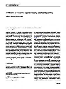
Figure 2.1 – Example of a phylogenetic tree (source: http://sites.duke.edu/dukeresearch/2011/11/14/ being-the-shy-kid-may-have-its-benefits/ and adapted from http://phylogenous.files.wordpress.com/2011/ 01/treea.png).

Phylogenetics is the study of evolutionary relationships among groups of organisms and phylogenetic trees are used to represent such relationships. There are three commonly used tree building frameworks to build phylogenetic trees using DNA sequence data: distance based, maximum parsimony, and maximum likelihood approaches [40]. Phylogenetic trees build on DNA or protein sequences are usually represented as binary trees, with leaf nodes representing the modern species and the ancestral nodes representing some ancestral species from which the modern species were derived. The branches (edges) of the tree represent number of evolutionary changes or evolutionary time. An example of a phylogenetic tree is shown in Figure 2.1.

2.1.3 Developmental biology and Evolution In developmental biology, the process by which a less specialized cell becomes a more specialized cell type is called cell differentiation [22]. During the development of a multicellular organism, differentiation occurs numerous times as the organism changes from a simple 6

2.1. Biological concepts zygote to a complex system of tissues and cell types. Cell differentiation almost never involves a change in the DNA sequence itself (with a few exceptions). Therefore since all cells in one individual organism have the same genome, epigenetic factors and transcriptional factors play an important role in cell differentiation [71, 75, 76]. For mammals, early development is characterized by the zygote becoming a ball of cells called blastocyst which later becomes embryonic stem cells. Embryonic stem cells are basically undifferentiated biological cells that can differentiate into specialized cells and can divide through mitosis to produce more stem cells [22].

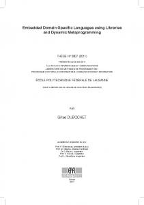
Figure 2.2 – Example of cell-differentiation among blood cells (source: Wikipedia). The arrows indicate a tree structure.

Cells of a multicellular organism are classified into cell types based on their morphological, physiological or molecular characteristics. Since cell differentiation transforms less specialized cell types into more specialized ones and since most specialized cells of one organ cannot be converted into specialized cells of some other organ, the paths of differentiation together form a tree, in many ways similar to the phylogenetic trees used to represent evolutionary histories. An example of tree structure among differentiation of blood cells is shown in Figure 2.2. In contrast to cell differentiation, evolution deals with changes taking place in the genome across species. We outline some of the similarities and differences between the fields of cell-differentiation and evolution. Some similarities are as follows: (1) In cell differentiation, more specialized cells are evolved from less specialized cells, while in evolution, present-day species have evolved from some ancestral species — so a tree representation is possible in both cases. (2) The observed changes in the epigenetic state are inheritable, again much as mutations in the genome are (although, of course, through very different mechanisms and at very different scales). As histone modifications are replicated in the cell-differentiation process we can 7

Chapter 2. Background assume not all histone modification marks are perfectly copied from parent to child, due to the stochastic nature of chemical reactions. Therefore there could be stochastic changes in epigenetic features. (Some plausible mechanisms of inheritance of histone modifications marks are given in [81, 132, 98].) (3) Epigenetic traits are subject to stochastic changes, just like genetic mutations. Some of the differences are: (1) The time scales may be very different, cell differentiation happens in a few days or weeks, while evolutionary time scales can be large (millions of years in the case of evolution of mammals). (2) While phylogenetic analysis places all the modern data at the leaves of a tree, with regard to cell differentiation some of the less specialized cell types may continue to exist in the organism and hence they could be ancestral nodes and not leaf nodes. (3) There are well defined models of evolution of DNA sequences for phylogeny while the models of differentiation for mutations in epigenetic states across cell types are not so well defined. In cell differentiation, the program of mutational events is itself the result of evolution, so as observed by Arendt [3], the cell differentiation tree often recapitulates the phylogeny of cell types. Thus keeping the similarities and differences between the fields of evolution and cell differentiation in mind, we used phylogenetic methods for the analysis of cell types using histone modification data to study cell differentiation. We call the trees we build as cell-type trees (details given in chapter 5). We also discuss the role of evolution of cell types and how cell-type trees can be used to study this phenomenon in chapter 5. The number of cell types in various organisms do vary. We discuss in chapter 5, how cell-type trees can be used to study the evolution of cell types when comparing the current species to some ancestral species.

2.2 Experimental technology and data 2.2.1 ChIP-Seq technology The current technology to capture histone modifications is chromatin immunoprecipitation (ChIP), which uses an antibody to isolate DNA fragments in contact with histones that carry a specific modification or transcription factors. ChIP-chip, ChIP-PET, and ChIP-SAGE are some of the ChIP-based technologies used for the study of histone modifications or transcription factor binding in genomic regions [57, 63, 123]. Thanks to advances in sequencing technologies, ChIP-Seq has become the main approach for capturing histone modifications and transcription factors, due to its high throughput, high resolution, and low cost [7, 59, 80, 66]. In the ChIP-Seq process, the sequence of one end of the DNA fragment is read to provide a tag which is then mapped to an assembled genome to determine the location of the DNA fragment. Various steps of the ChIP-Seq process are shown in Figure 2.3.

8

2.2. Experimental technology and data

Figure 2.3 – The various steps in the ChIP-Seq procedure are shown (source Wikipedia).

2.2.2 Common data formats The ChIP-Seq process gives us a collection of fragments whose ends are sequenced (tags) and mapped back into the genome, the data we get is usually represented as a collection of 9

Chapter 2. Background fragments with chromosome no., starting and ending position in the chromosome (base pair resolution). The common data formats are BED or BAM. The first three required BED fields are: chrom - The name of the chromosome (e.g. chr1, chrY). chromStart - The starting position of the feature in the chromosome. chromEnd - The ending position of the feature in the chromosome. There are 9 additional optional BED fields. The sixth position usually signifies the positive (+) or negative strand (-). BAM is the compressed binary version of the Sequence Alignment/Map (SAM) format, a compact and index-able representation of nucleotide sequence alignments. More details of the formats are given in the UCSC Genome Browser http://genome.ucsc.edu/FAQ/FAQformat. html.

2.2.3 Data availability The most common sources of data for histone modifications are ENCODE project [82], Roadmap Epigenomics project, Gene Expression Omnibus (GEO) repository.

2.2.4 Data visualization The UCSC genome browser is often used to visualize the data [61].

2.3 Computational Methods 2.3.1 Data representation One of the common ways to represent the ChIP-Seq data, is by dividing the genome into non-overlapping windows (called bins) and collecting, for each bin, a count of the mapped sequence tags that fall within the bin (called bincount). Thus we get a “library", which is simply a list of non-negative integers, each successive integer associated with the next bin. Since the median length of each histone modification ChIP-Seq fragment is about 200 bp [7, 99], one can approximate the center of each fragment by shifting the tag end position by 100 bp (or so) downstream or upstream, according to its orientation on the chromosome, as done in [125]. (We note that for paired-end data the fragment length distribution is known and for single-end data the fragment length distribution can be inferred from an autocorrelation analysis. Knowledge of this distribution may be important for proper normalization and data processing.) We also use the word “library” for other forms of data representation of ChIP-Seq data too. Now these ChIP-Seq libraries are used for statistical analysis. A hand-drawn example of a

10

2.3. Computational Methods

Genome

Peak

Peak

Figure 2.4 – Profile of a ChIP-Seq data library. Signal above some threshold are classified as peaks.

ChIP-Seq data library is shown Figure 2.4. The regions of the genome where the signal falls above some threshold are classified as peak regions.

differential regions

L1

L2

Figure 2.5 – Profile of two ChIP-Seq data libraries L1 and L2. Differential regions in the genome are marked.

Another hand-drawn example showing two ChIP-Seq libraries L1 and L2 is shown in Figure 2.5. Regions of the genome where L1 is significantly enriched when compared to L2 or vice-versa are called differential regions. The problem of detecting such differential regions is what we address in chapter 3. A real example of a ChIP-Seq library as visualized in the UCSC Genome Browser is shown in Figure 3.1. 11

Chapter 2. Background

2.3.2 Statistical measures Some of the statistical measures used in this thesis are given below.

Fold change threshold Fold change thresholds have been used in literature to determine which regions are enriched when comparing ChIP-Seq data from two different cell types. In [125], a fold-change threshold value of 3 was used. We used a fold change threshold for our work in chapter 3.

False discovery rate False discovery rate (FDR) [9] is a statistical measure which is used in multiple hypothesis testing to correct for multiple comparisons. For the ChIPnorm method we binned the ChIPSeq data into various bins. FDR estimation is done to find which bins are significantly enriched P E (t ) nul ≥t or not. FDR is estimated as F DR(t ) = P E obsl(t ) [94], where E obs (t ) is the number of observed ≥t bins which have bincount values ≥ t and E nul l (t ) the number of expected bins which have bincount values ≥ t . The FDR threshold which is often used in literature is 0.05. More details are given in [94].

p-value In statistical significance testing, p-value is the probability of obtaining a test statistic result at least as extreme as the one that was actually observed, assuming that the null hypothesis is true [48, 49]. The null hypothesis is rejected if the p-value turns out to be less than a predetermined significance level, often 0.05 [117, 25] or 0.01. p-values are often used to show the significance of ChIP-Seq peaks. The smaller the p-value (or greater the negative log p-value), the more significant the peak is. We use p-values when using the peak data in chapter 5. In the multiple testing problem it may be better to use a tighter p-value threshold so that we do not get a large number of false positives by chance alone. Therefore it is better to adjust the p-values using an optimized FDR approach. the adjusted p-value is called a q-value in literature. More details of this can be found in [118, 119].

IDR Reproducibility is important for high throughput experiments to be considered reliable. Irreproducible discovery rate (IDR) framework is a unified approach to measure the reproducibility of findings identified from replicate experiments. Unlike the usual scalar measures of reproducibility, the IDR approach creates a curve and quantitatively assesses when the findings are no longer consistent across replicates. The IDR score can be computed at each set of paired replicate ranks and permits the principled setting of thresholds both for assessing reproducibility and combining replicates [73]. The paper [73] reproducibility is described as the 12

2.3. Computational Methods extent to which the ranks of the signals are no longer consistent across replicates in decreasing significance. The authors of that paper propose a copula-based graphical tool to visualize the loss of consistency and localize the possible breakdown of consistency empirically. After that reproducibility is quantified by classifying signals into a reproducible and an irreproducible group, using a copula mixture model. Their model then assigns each signal a reproducibility index (which estimates its probability to be reproducible) by jointly modeling the significance of scores on individual replicates and their consistency between replicates. Then based on this index, they define the irreproducible discovery rate (IDR) and a selection procedure, in a fashion analogous to their counterparts in multiple testing, to rank and select signals [73]. IDR is intended to be analogous to FDR [73]. We use some IDR analysis for our work in chapters 4 and 5.

2.3.3 Normalization techniques Data normalization techniques are very important for us to compare data arising from two different experiments. There are many normalization techniques present in literature, the simplest of those being mean normalization, standard score normalization. Quantile normalization is one such normalization technique used in statistics, for making two distributions identical in statistical properties. Quantile normalization has often been used in microarray data analysis [1, 16]. One way to do quantile normalization on a test distribution to a reference distribution of the same length is to sort the test distribution and sort the reference distribution; then the highest entry in the test distribution takes the value of the highest entry in the reference distribution, the next highest entry in the reference distribution, and so on, until the test distribution is a perturbation of the reference distribution. If we wish to do quantile normalization on two or more distributions to each other, without a reference distribution, sort as before, then set to the average (usually, arithmetical mean) of the distributions. Now the highest value in all cases becomes the mean of the highest values, the second highest value becomes the mean of the second highest values, and so on. We have adapted the quantile normalization method and used it on ChIP-Seq data (chapter 3).

2.3.4 Expectation-maximization algorithm The expectation-maximization (EM) algorithm [28] is an iterative method for finding maximum likelihood or maximum a posteriori (MAP) estimates of parameters in statistical models, where the model depends on unobserved latent variables or missing data. The EM algorithm alternates over two steps: guessing a probability distribution over completions of missing data given the current model (known as the E-step) and then re-estimating the model parameters using these completions (known as the M-step). The name ‘E-step’ comes because one does not usually need to form the probability distribution over completions explicitly, but rather need only to compute ‘expected’ sufficient statistics over these completions. Also the name ‘Mstep’ comes because model re-estimation can be thought of as ’maximization’ of the expected 13

Chapter 2. Background log-likelihood of the data [31]. EM algorithms are widely used in many areas of computational biology [31], like gene expression clustering [30], motif finding [70], haplotype inference problem [37], learning profiles of protein domains [64] and RNA families [34], discovery of transcriptional modules [108], tests of linkage disequilibrium [112], genome segmentation [54], protein identification [92] and medical imaging [27], etc. We have used an EM framework for our probabilistic partitioning approach given in chapter 4.

2.3.5 Phylogenetic tree building methods Three of the most commonly used phylogenetic tree building framework are: using distance based, maximum parsimony, and maximum likelihood approaches [40]. Some details of each approach are outlined below.

Distance based methods Distance based methods or distance matrix methods were introduced in [35] and [43]. They were influenced by the clustering algorithms of Sokal and Sneath [113]. The general idea of distance based measures is to calculate a measure of distance between each pair of species, and then find a tree that predicts the observed set of distances as closely as possible [40]. A multiple sequence alignment (MSA) of the DNA or protein sequences are given as input to the distance based algorithms. One of the most commonly used distance based method is the neighbor-joining algorithm [104]. It takes the distance matrix, specifying the distance between each pair of taxa, as an input. The algorithm starts with completely unresolved tree (star shaped) and iteratively follows a series of steps till the tree is resolved and all branch lengths are known. The simple neighbor-joining method produces unrooted trees. (A rooted phylogenetic tree is a directed tree with a unique node corresponding to the the most recent common ancestor of all the entities at the leaves of the tree. Unrooted tree is tree without a root.) It does not assume a constant rate of evolution (i.e. a molecular clock) across lineages. Unlike the neighbor-joining method, its relative called the UPGMA (Unweighted Pair Group Method with Arithmetic Mean) which is simple agglomerative (bottom-up) hierarchical clustering method produces rooted trees and requires a constant-rate assumption - that is, it assumes an ultrametric tree in which the distances from the root to every branch tip are equal [114, 40]. Since the UPGMA assumes the molecular clock hypothesis (constant rate of evolution), it is not a well-regarded method for inferring relationships unless this assumption has been tested and justified for the data set being used. The use of neighbor-joining method is thus seen as an advantage as it does not make the molecular clock assumption. The other important feature of neighbor-joining and most other distance based methods is that they are polynomial-time algorithms and are very fast. Neighbor-joining tree also has the property 14

2.3. Computational Methods that if the input distance matrix is additive, then the output tree will be a unique correct tree. That is, the distance between any two leaves of the tree is given by the sum of the edges of the path connecting them and it will be same as the corresponding number in the given additive matrix. Also if the distance matrix is “nearly additive”, that is if each entry in the distance matrix differs from the true distance by less than half of the shortest branch length in the tree, then the correctness of the output tree topology given by neighbor-joining method is guaranteed [4]. Although the distance matrix rarely satisfies this condition, it has been seen that neighbor-joining quite often constructs the correct tree topology anyway [84]. We have used neighbor-joining approaches in building cell-type trees in chapters 5 and 6.

Maximum parsimony based methods Maximum parsimony methods were among the first methods used for inferring phylogenies and their general idea was first described in [35] which declared that the evolutionary tree is to be preferred that involves “the minimum net amount of evolution”. Maximum parsimony predicts the evolutionary tree or trees that minimize the number of steps required to generate the observed variation in the sequences from common ancestral sequences [86]. Therefore this method is also sometimes called minimum evolution method. Maximum parsimony methods are more time consuming and finding the most parsimonious tree is an NP-Hard problem [26]. However given a fixed tree, the Fitch’s algorithm (a dynamic programming approach) can be used to compute the parsimony score and the states of the internal nodes in polynomial time (small parsimony problem) [42]. In some datasets, maximum parsimony methods are found to be better than distance based approaches. The software TNT is a popular parsimony based method to find a phylogenetic tree [47]. We have also used maximum parsimony approaches in building cell-type trees in chapters 5 and 6.

Maximum likelihood based methods The maximum likelihood method uses underlying probabilistic model on a set of observed sequences and outputs a tree which maximizes the likelihood of the data [121, 40]. The likelihood of the data is basically the conditional probability of producing the data given the model parameters. Usually a substitution model is the probabilistic model used. Maximum likelihood uses a probability of base substitution per evolutionary unit. Maximum likelihood based methods are found to computationally time consuming but usually more accurate than distance based or maximum parsimony based methods [45]. RAxML is a popular method to find phylogenetic tree using a maximum likelihood framework [116].

2.3.6 Minimum spanning tree Spanning tree of a given connected undirected graph is an acyclic subgraph which connects all the vertices together. Typically there are multiple spanning trees in a single graph. There could

15

Chapter 2. Background be weights assigned to each edge. The sum of the weights of all the edges in that spanning tree gives the weight of the spanning tree. A minimum spanning tree (MST) is a spanning tree with weight less than or equal to the weight of every other spanning tree. Two very common algorithms to find a MST are Prim’s algorithm [97] and Kruskal’s algorithm [65], both of which are greedy algorithms. We have used MST method in chapter 6.

16

3 ChIPnorm: a statistical method for normalizing and identifying differential regions in histone modification ChIP-Seq libraries

3.1 Introduction As we have seen in the earlier chapters, histones are proteins that package the DNA into nucleosomes [72]. These histones are subjected to various types of modifications which alter their interaction with the DNA and nuclear proteins, thereby influencing transcription and genomic function. These modifications along with other epigenetic marks help us understand why various types of cells exhibit very different behaviors in spite of their shared genome. Thus the study of histone modifications, and more particularly of the differential enrichment of these modifications in different cell types, is a crucial tool in the understanding of genomic function. Because of the advances in sequencing technologies, ChIP-Seq has become the main approach for capturing histone modifications, due to its high throughput, high resolution, and low cost [7, 59, 80]. In the ChIP-Seq process, there is first the chromatin immunoprecipitation (ChIP) step, which uses an antibody to isolate DNA fragments in contact with histones that carry a specific modification or transcription factors. Then the sequence of one end of the DNA fragment is read to provide a tag which is then mapped to an assembled genome to determine the location of the DNA fragment. Genome-wide chromatin maps (using ChIP-Seq technology) for three mouse cell types— embryonic stem (ES) cells, neural progenitor (NP) cells, and embryonic fibroblasts (EF) — have been published [85]. The authors of the paper compared the occurrence of histonemodification sites in promoter regions of the three cell types in a qualitative manner. Subsequently, the first quantitative comparison of two ChIP-Seq libraries using computational techniques appeared [125]; there the authors addressed the problem of finding differential regions given two histone-modification libraries for two different cell types. Their method, 17

Chapter 3. ChIPnorm: a statistical method for normalizing and identifying differential regions in histone modification ChIP-Seq libraries ChIPDiff, is based on hidden Markov models. Recently, Taslim et al. 2009 [122] proposed a two-step nonlinear normalization method based on locally weighted regression (LOESS) [20] to compare ChIP-Seq data across multiple samples; they modeled the difference using an exponential-normalK mixture model, then used this fitted model to identify genes associated with differential binding sites. This method first normalizes the data using a locally weighted polynomial least square regression to estimate a LOESS smoother of the mean and variance of the observed data. After normalization they fit a finite mixture model to the normalized data and perform model-based classification to identify genes associated with enrichment regions. The assumption used in the mixture model is that the data comes from three (non-differential, positive- and negative-differential) groups. The non-differential regions are assumed to come from a mixture of K -component normal distributions, where K is unknown and needs to be estimated from the data. The assumption used is that the positive- and negative-differential regions follow exponential and the mirror of exponential distributions, respectively [122]. Using the fitted model they identify genes associated with differential binding sites based on local false discovery rate. However we would like to identify differential regions not just on genes but throughout the genome. Another recent method is RSEG [115]. RSEG identifies epigenomic domains from ChIP-Seq data for histone modifications and is based on hidden Markov model (HMM) framework including the Baum-Welch training and posterior decoding. The method is also able to incorporate a control sample and find genomic regions with differential histone modifications between two samples. From a mathematical viewpoint the problem of finding genomic regions with differential histone modifications between two tissues is not fundamentally different from that of peak finding in ChIP-Seq data using an input control to correct for technical biases. Many such peak finders have been proposed [131]. Some of the other methods present in literature for differential analysis for ChIP-Seq data are DESeq [2], DBChip [74]. The DESeq method assumes the number of reads in a sample that are assigned to a gene can be modeled by a negative binomial distribution, and then the model is fitted to data. This method again works only for finding differential genes and not for all regions in the genome. DBChip is mainly meant for transcription factor ChIP-Seq data. Even after the work done by us in this chapter, some new literature regarding differential analysis has come up in literature. One such method is called MMDiff [107] which detects differential regions taking into account any shape changes of the signals. MMDiff is a multivariate non-parametric approach to testing significant differences in profile patterns between peaks in different conditions and it exploits higher order features in the peak shapes. A significant impediment to the analysis of ChIP-Seq data is the high level of noise. Noise or systematic distortion can enter at various stages of the procedure: variations in the number of cells used in the experiment, variation in the amount of antibody that attaches to the DNA fragments, tandem repeats, uneven rates of success in sequencing different fragments, etc. The type of histone modification and the cell types can also affect the level of noise. For example, we show in this chapter that histone modification H3K27me3 (K27) in ES cells has less background noise and a better signal-to-noise (S/N) ratio than the same modification in NP cells. In addition, the signal tends to be found mostly in gene-rich regions of the genome. Therefore

18

3.2. Methods computational methods may produce many false positives. In the case of modification K27 for ES and NP cells, for instance, false positives are likely in gene-poor regions for NP cells and in gene-rich regions for ES cells. Such bias problems are present in microarray data and many authors have addressed this issue [33]. Similar studies are needed in ChIP-Seq data, as the data characteristics differ [19]. To address the problems of noise and bias in finding differential regions, we propose a twostage statistical method, called ChIPnorm [88], to remove the noise and the bias from two ChIP-Seq libraries and to normalize the data so as to enable a direct comparison between the two libraries to identify differential regions. Our normalization step is similar to quantile normalization [16]; however we have simplified the method so that it can be readily extended for normalization of more than two libraries. Our method is computationally efficient and can be applied to very large datasets. We use it to analyze ChIP-Seq histone modification data from different types of mouse and human cells, confirming previous findings and making some new observations. We also point to the usefulness of our approach to study histone modification data from Arabidopsis in the context of leaf senescence.

3.2 Methods To motivate our work, we examine data for histone modification H3K27me3 (K27) in mouse ES and NP cells [85]. Figure 3.1 displays a window of the data mapped onto the mouse genome through the UCSC genome browser [61]. ES data has better S/N ratio as well as more peaks in gene-rich regions than in gene-poor regions (as seen visually from Figure 3.1 and quantitatively from Figure 3.7). These characteristics introduce a bias that must be eliminated before comparing ES data to NP data, as can be seen in the results of the ChIPDiff method [125] in the same figure: most of the differentially NP enriched regions proposed by ChIPDiff fall within gene-poor regions and are almost certainly false positives. In the following, we use a notation similar to that of Xu et al. 2008 [125]. In particular, we assume that the data has been processed by dividing the genome into bins and collecting, for each bin, a count of the mapped sequence tags that fall within the bin. The result is a “library", which is simply a list of non-negative integers, each successive integer associated with the next bin. Let L a and L b be two libraries containing the same histone modification for two different cell types—in our example, modification K27 for ES and NP cell types. Let m be the total number of bins in the library and set Y a = {y ai |1 ≤ i ≤ m} and Yb = {y bi |1 ≤ i ≤ m} to be the observed counts of the ChIP-Seq fragments for libraries L a and L b respectively, where y ai , respectively y bi , are the sum of the fragments lying in the i th bin. In ChIP-Seq, a tag is retrieved by sequencing one end of the ChIP fragment, and the median length of this fragment is around 200 bp [7, 99]. As was done in Xu et al. 2008 [125], we approximate the center of each fragment by shifting the tag end position by 100 bp downstream or upstream, according to its orientation on the chromosome. (We note that instead of using a fixed value like 100 bp to approximate the center of each fragment, one could also infer a proper value separately for

19

Chapter 3. ChIPnorm: a statistical method for normalizing and identifying differential regions in histone modification ChIP-Seq libraries 2 Mb Scale chr1: 44500000450000004550000046000000465000004700000047500000480000004850000049000000495000005000000050500000 30 K27_mouse_ESC_1000 0_ 30 K27_mouse_NPC_1000 0_ ChIPnorm ChIPDiff DHMS UCSC Genes

Figure 3.1 – Histone modification profile as seen in the UCSC genome browser [61]. Tracks 1 (red) and 2 (green) show the H3K27me3 modifications for ES and NP cells, respectively. Track 3 shows the differentially enriched regions found by our ChIPnorm method. Track 4 shows the differentially enriched regions found by the ChIPDiff method [125]. In tracks 3 and 4, red indicates differential enrichment in ES cells and green indicates differential enrichment in NP cells. Track 5 shows the UCSC genes.

each dataset — however for simplicity we choose a fixed value of 100 bp for this work.) We choose different bin sizes for different types of the histone modifications so as to maximize the discriminative information between the two libraries of the different cell types and minimize the discrimination of the two replicates of the same libraries. We use the spread of the data in the scatter plots as a measure for discriminative information. A lower bin size favors a better spread (away from the diagonal) between the data of the two cell types in the scatter plot. (For robustness studies we also tried using a range of bin sizes, as shown in results section.) An observed fragment count y ai at the i th bin can be related to the actual number of histone modifications x ai at the i th bin using the following model: y ai

=

g a (x ai ) + εai + νai

y bi

=

g b (x bi ) + εbi + νbi

(3.1)

Function g is the (unknown) deterministic function that describes the nonlinear transformation of the actual histone modifications, accounting for the various experimental conditions that may influence the observations in a systematic way. The additive ε term accounts for the stochastic (background) noise introduced by the experimental setup, such as stray fragments from neighbouring modifications. Finally, the parameter ν accounts for local genomic bias, mainly bias due to open chromatin regions and mapability, such noise is common in both the actual ChIP-Seq library and the corresponding control dataset. Naturally, one could choose a stochastic, rather than a deterministic model for g ; but since our goal is to detect regions with differential enrichment, and not to produce a detailed predictive model, the deterministic approach suffices. 20

3.2. Methods

3.2.1 ChIPnorm scheme We will address each source of error separately and proceed in two main stages. In the first stage, we address the removal of stochastic background noise and local genomic bias in each library. In the second stage, we address the problem of normalization.

3.2.2 Stochastic noise ε To solve the problem of stochastic background noise, both Bayesian modelling methods [36] and statistical confidence measure methods have been used. In terms of statistical confidence, the problem reduces to evaluating the probability that a particular bincount (bincount is the total number of DNA fragments captured inside a bin of some size) would occur by chance [94]. We estimate this probability by defining a “null hypothesis”, which is a random distribution of bincounts, and then comparing it with the distribution of bincounts of the ChIP-Seq library. To understand the rationale for choosing the amplified binomial distribution (ABD) as the random distribution for the bincounts of ChIP-Seq library, we must examine the ChIP-Seq process as illustrated in Figure 3.2. The short segments of DNA are treated with a specific antibody to capture a particular histone modification in the genome. The rest of the fragments are washed away. The captured fragments are sequenced by a high-throughput sequencing method, which typically uses PCR amplification of the captured fragments [52] before performing the final base-pair sequencing. The sequenced data is binned to obtain a ChIP-Seq library. To estimate the null distribution of a ChIP-Seq library, we assume that the fragmented DNA from the sonicated whole cell is treated with an antibody that randomly captures fragments without any specificity. The bincounts of captured fragments then follow a binomial distribution. The captured fragments are amplified, sequenced, and binned to get the null distribution of the ChIP-Seq library. This binned data follows a random distribution, in which each of the fragments following the binomial distribution is amplified; we refer to it as the amplified binomial distribution (ABD). We assume that each fragment is amplified by a constant amplification factor. An ABD can be defined by two parameters: the total number of fragments Nbi no in its corresponding binomial distribution and the amplification factor α. We made two assumptions to calculate these parameters for the desired null distribution: (a) the total number of the fragments in the original ChIP-Seq data Nd at a and in the corresponding null distribution Nnul l = α×Nbi no are the same, and (b) the total number of bins with zero bincount is the same in the ChIP-Seq library (Zd at a ) and the null distribution. Since the amplification does not ¡ ¢N change the number of bins with bin-count zero, we can write Zbi no = Zd at a = 1 − B1 bi no B , where B is total number of bins in the library. Since Zd at a and B are observed variables, Nbi no d at a and α = N Nbi no can be evaluated. Now the probability mass function of the random distribution

21

Chapter 3. ChIPnorm: a statistical method for normalizing and identifying differential regions in histone modification ChIP-Seq libraries

Figure 3.2 – Overview of ChIP-Seq process. We see how we can get the ChIP-Seq library, input DNA control, and the random distribution (null hypothesis).

prior to amplification is Ã

Nbi no P r and om (t ) = t

!µ ¶ µ ¶ 1 t 1 Nbi no −t 1− , 0 ≤ t ≤ Nbi no . B B

The ABD is thus estimated as P AB D (t ) = P r and om (t /α). The estimated real distribution of the original ChIP-Seq data for one chromosome is shown in Fig. 3.3 (blue). An example of random distribution (amplified binomial distribution with α = 2) is also shown (red). The figure is zoomed into a small region for clarity. We can see that since the number of zero bins are same, the probability that bincount is 0 is same for both. The random distribution tends to have a higher probability than real distribution at lower bincounts but a lower probability at higher bincounts. We calculated the false discovery rate (FDR) for a ChIP-Seq data using its corresponding estimated null distribution (ABD) [94]. We declared bins with FDR ≤ 0.05 as significant bins in the ChIP-Seq library. The value 0.05 is the standard value used in the field [94]. 22

3.2. Methods

0.4

ABD Data probability

0.35

Probability −−>

0.3 0.25 0.2 0.15 0.1 0.05 0 0

5

10

bincount −−>

15

20

25

Figure 3.3 – An example of random distribution (amplified binomial distribution with α = 2) is shown in red and the estimated real distribution of the original ChIP-Seq data for one chromosome is also shown (blue). ABD — amplified binomial distribution. Data probability — estimated real distribution. The figure is zoomed into a small region for clarity.

3.2.3 Local genomic bias ν ChIP-Seq data contains many local genomic biases corresponding to open chromatin regions, over-amplified satellite repeats, GC-rich regions, and unmappable perfect repeat regions. Some of these biases depend on experimental conditions and others may vary among the cell lines in a systematic manner. If such cell-specific biases are not taken care of while comparing ChIP-Seq libraries it will give many false positive differential regions. Some of these biases can be reduced by using an input DNA control library. To find differential regions, we must consider only those regions that are significantly enriched with respect to the input DNA control. The input DNA control are the DNA fragments in the ChIP-Seq experiment prior to the application of the histone specific antibody. To find the enriched bins, we need to normalize the input DNA control with respect to the data. Yang et al. 2002 [127] recommended the use of locally weighted regression (LOESS) normalization. The basic assumption is that the percentage of the differential sites, considered as outliers by LOESS, is small so that these sites do not affect the normalization. However, this is not true in the case of a ChIP-Seq library. In a ChIP-Seq library, the percentage of bins that are differentially enriched relative to the input DNA control can exceed 50%. These differentially enriched bins will affect the LOESS normalization as shown in Figure 3.4(a) and lead to many false negatives. We introduce an iterative normalization to overcome this problem. In the first stage of iterative normalization, we normalize the DNA control with respect to the data using quantile normalization. For illustration purposes, we first show the LOESS curve of the MA plot in 3.4(a). (MA plot is often used for visual representation of two channel DNA microarray gene expression data [33] which has been transformed onto the M (log ratios) 23

Chapter 3. ChIPnorm: a statistical method for normalizing and identifying differential regions in histone modification ChIP-Seq libraries

(a) 8

Log(data) − Log(control)

MA 6

MA (smooth)

4

fit 1

2 0 −2 −4 −6 −8

(b)

2

4

6

8

10

12

14

1/2(Log(data) + Log(control))

Figure 3.4 – Iterative Normalization of input DNA. (a) before first iteration. (b) after first iteration, post removal of outliers.

and A (mean average) scale.) We first classify bins enriched with respect to the DNA control (fold change > 1) after quantile normalization as outliers. These outliers are then removed from further iterations. Figure 3.4(b) shows the LOESS curve after removing the outliers. We see that the LOESS curve is relatively less affected by outliers. In the next iteration, we use non-outliers bins for second quantile normalization to get a more accurate estimate of the normalization function. Once we get this normalization function, we normalize (quantile) all bins. The process of removing outliers and then performing normalization can be repeated to rescue more bins falsely declared as non-enriched. Each bin is declared as enriched if its fold-change value of ChIP-Seq data and quantile normalized control data is > 1. (The LOESS normalization is not used in the ChIPnorm method but is shown here only for illustrating the affects of normalization and removing outliers. Instead quantile normalization is used.) Bins which are declared both as significant in the ABD approach and as enriched in the iterative approach, are declared as ‘enriched-significant’. Bins which are declared as enrichedsignificant in either of the two libraries are passed on to the second stage, with their original bincount values.

3.2.4 Quantile normalization Since our first stage removed the majority of bins with low S/N ratios and genomic bias, and since we expect interesting regions to have good S/N ratios, we make the simplifying 24

3.2. Methods assumption: εai

= εbi = 0

νai

= νbi = 0;

(3.2)

With this assumption the next step is to normalize the data to the same scale so that bin values in the two libraries are comparable. We propose a quantile normalization method (similar to Bolstad et al. 2003 [16]) to solve this normalization problem. Quantile normalization assumes that the distribution of the data of the two libraries that are being compared are similar. This may seem problematic because histone modifications change significantly during differentiation. But it is reasonable to assume that their probability distribution of the bincount over the whole genome is similar across different cell types. (This might not be true if one of the two libraries have histone modifications knocked out. This may also not be a valid assumption if the development stage includes a major redistribution of a given histone modification, for example the marking or unmarking of large portions of the genome.) We formulate the problem mathematically as follows. Given two observed data y ai = g a (x ai ) and y bi = g b (x bi ), ∗ find a transformation f ∗ = (g a ◦ g b−1 ) such that y bi = f ∗ (y bi ) = g a (x bi ). We make the following assumptions: – The actual histone modifications X a = {x ai | i ∈ {1, m}} and X b = {x bi | i ∈ {1, m}} follow the same distribution, i.e., we have F X a (x) = F X b (x). – Cumulative distribution functions (cdf) F X a and F X b are monotonically increasing. – g a ( ) and g b ( ) are monotonically increasing. The last two conditions imply that F Ya and F Yb are also monotonically increasing. Theorem 1 Any function fˆ : y bi → yˆbi satisfies F Yˆb (y) = F Ya (y) if and only if we have fˆ = f ∗ . Lemma 1

F Yb∗ (y) = F Ya (y)

Proof (of lemma): F Ya (y) = P (Y a ≤ y) = P (g a (X a ) ≤ y) = P (X a ≤ g a−1 (y)) = F X a (g a−1 (y)) and F Yb∗ (y) = P (Yb∗ ≤ y) = P (g a (X b ) ≤ y) = P (X b ≤ g a−1 (y)) = F X b (g a−1 (y)) = F X a (g a−1 (y)) Proof (of theorem): only if part: if we have fˆ = f ∗ , then from Lemma 1, we also have F Yˆb (y) = F Yb∗ (y) = F Ya (y). if part: if we have F Yˆb (y) = F Ya (y), then from Lemma 1, we also have F Yb∗ (y) = F Yˆb (y). Additionally, as cdfs are assumed to be monotonically increasing, they are one-to-one functions. ∗ Hence we can write ∀i , yˆbi = y bi , which in turn implies fˆ = f ∗ .

25

Chapter 3. ChIPnorm: a statistical method for normalizing and identifying differential regions in histone modification ChIP-Seq libraries 150

Histone modification count

ES NP

100

50

0 0

10

20

30

40

50

60

70

80

90

100

Percentile

Figure 3.5 – The new inverse cumulative distribution function on the modified libraries (after stage 1). On the x axis is the percentile, on the y axis are the bin values.

Theorem 1 states that if (i) we have F X a (x) = F X b (x), (ii) the cumulative density functions of X a and X b are identical and monotonically increasing, and (iii) g a ( ) and g b ( ) are deterministic monotonic increasing functions, then any transformation that meets the conditions of the theorem is our desired transformation f ∗ = (g a ◦ g b−1 ). To find such a transformation, we use the inverse cumulative distribution function (on the modified data after removing noisy bins) of the enrichment level, as shown in Figure 3.5. The x axis of this figure is the percentile while the y axis is the bin values. The figure shows the L a and L b bin values plotted against their cumulative percentile. To get the desired transformation of Yb , we must ensure that the post-transformation data Yˆb follows the same cdf as Y a . We fit a spline smoothing function on the bin values of library L a , then, for all percentile values p, we perform a transformation fˆ : y b → yˆb such that yˆb (p) = y a (p). The transformation fˆ ensures that the conditions of Theorem 1 are met. This transformation reduces the problem of comparing two libraries with different probability distributions to the problem of comparing two libraries following the same probability distribution, so that a direct comparison of values can now be used. Since in the second stage we considered bins which were declared as enriched-significant in either of the two libraries L a and L b (a union operation), some bins which are not declared as enriched-significant would be present in the second stage too. If both libraries were completely independent events, we would expect 50% of the bins to be enriched-significant, because of the union operation. In effect, we define a bin in library L b to be differentially enriched for the target modification if (i) observed bin value in libraries L b lies above the 50% region in the inverse cumulative distribution function and (ii) for some chosen fold change threshold τ (> 1), we have yˆbi /y ai ≥ τ. Similarly we can define a bin in library L a as differentially enriched if the bin value in library L a lies above the 50% region in the inverse cumulative distribution function and for for some chosen threshold τ (> 1), we have y ai / yˆbi ≥ τ. All bins are thus reported as differentially enriched or not. Adjacent bins of the same type of differential enrichment can be 26

3.2. Methods grouped together to form differential regions (DHE).

3.2.5 The complete ChIPnorm method summarized The complete ChIPnorm method is summarized in the Figure 3.6. In the first stage, we identify bins having a significant bincount compared to the estimated random distribution of a ChIPSeq library as significant bins, by using a false discovery rate (FDR) analysis. We also identify bins of a ChIP-Seq library as enriched bins, if their bincounts are higher than the corresponding bincounts of the normalized input DNA control. Those bins which are both significant w.r.t. null hypothesis and enriched w.r.t. normalized input control DNA are declared as enrichedsignificant bins. Bins which are declared as enriched-significant in either of these two libraries are passed to the second stage. In the second stage, we normalize the enriched-significant bincounts of the two ChIP-Seq libraries and use a fold change to obtain differentially enriched bins. STAGE 1 Estimated random distribution

ChIP−seq bins

Input DNA (control) bins

FDR

Iterative normalization

Significant bins

Enriched bins

Enriched significant bins STAGE 2 Library 2 enriched significant bins

Library 1 enriched significant bins

Normalization

Differentially enriched bins

Figure 3.6 – The schematic diagram of the ChIPnorm method. In the first stage one we find the enriched-significant bins by removing various kinds of errors in the data. In the second stage we normalize the two ChIP-Seq libraries and find differentially enriched bins.

The normalization can also be used to find bins that are enriched in both libraries, thereafter called constitutively highly enriched (CHE). Bins which are above 50% in L a and L b in the 27

Chapter 3. ChIPnorm: a statistical method for normalizing and identifying differential regions in histone modification ChIP-Seq libraries inverse cumulative distribution function and also below threshold τ are declared as CHE. While differential histone modification enrichment (DHE) regions help us understand why different types of cells behave differently, CHE regions are conserved between the cell types and thus presumably essential to the survival of both types. The normalization method also facilitates the comparison of more than two libraries. Our method is easily extended to handle multiple types of histone modifications in multiple cell types. Such analyses can give more insight into combinatorial patterns of histone modifications, sometimes referred to as “histone language" [120]. For example, Bernstein et al. 2006 [11] hypothesized that a bivalent domain with both H3K27me3 and H3K4me3 modification at the same site plays a crucial functional role in embryonic stem cells. Finally, the ChIPnorm method can be used with any ChIP-Seq data—not just with histone modifications.

3.3 Experimental Design We carried out a series of experiments with the two libraries for H3K27me3 and H3K4me3 histone modifications (ES and NP cells), including experiments for bias and sensitivity. Since H3K4me3 has sharper peaks than H3K27me3, it needs a finer resolution, and smaller bin sizes are used. Using the replicate data analysis described earlier, we chose a bin size of 1000 bp for H3K27me3 (K27) and a bin size of 200 bp for H3K4me3 (K4). The bin size of 1000 bp for H3K27me3 has also been used previously in literature [125]. We compared ChIPnorm with six other normalization methods: (a) unit mean normalization; (b) quantile normalization; (c) MACS peak finder; (d) ChIPDiff method [125]; (e) rank normalization; and (f) two-stage unit mean normalization. We ran these methods on the H3K27me3 data for ES and NP mouse cells provided by Mikkelsen et al. 2007 [85] (with whole cell extract (WCE) control library) and on the H3K27me3 data (of Broad Institute) for ES and GM12878 (replicate 1) from the human ENCODE project [13, 100]. (GM12878 is a lymphoblastoid cell line produced from the blood of a female donor with northern and western European ancestry by EBV transformation [13].) Processing was done on individual chromosomes of the two libraries. The five methods not yet described are as follows: – unit mean normalization: is the standard Affymetrix scaling method for microarray data [16]. To perform consistent comparison with the ChIPnorm method, we normalized the two libraries to have unit mean using a method similar to the Affymetrix scaling method. To normalize the bin values x i of a library we calculated its trimmed mean x¯ (the mean of the ¯ Finally a non-zero bins in the library) and then the normalized bin value is set to x i0 = x i /x. threshold (τ) was used to classify bins as differential or not. – quantile normalization: the two libraries are quantile normalized, and a fold change threshold (τ) is used to classify bins as differential or not. – MACS peak finder method: Although MACS is a peak-finding software [131], we use it indirectly to find differential regions as follows: peaks for one library are detected by giving the other library as control, and the bins with peaks are considered as differential regions.

28

3.4. Results The version of MACS software used is “macs14 1.4.1 20110622”. – rank normalization: the bin values of each of the libraries are sorted separately; the sorted lists are divided into 10 equal partitions, which we define as rank. Finally we compare the values of corresponding ranks at each bin value in both libraries. If the difference between the values is greater than a threshold ν then the bin is classified as differential. – RSEG method: RSEG is a recently published method [115] to not only find peaks in histone modifications but to also identify differential regions (rseg-diff) between two histone modification ChIP-Seq libraries. – two-stage unit mean normalization: we removed the noisy bins using the first stage of the ChIPnorm method before applying the unit mean normalization and fold change classification. For methods unit mean normalization, quantile normalization, rank normalization, two-stage unit mean normalization, ChIPnorm, the fold change ratios where calculated by adding +1 on the numerator and denominator before calculating the ratio so as to avoid the divide-by-zero case. For the sensitivity analysis using the ENCODE data the corresponding gene expression data (RPKM - Reads Per Kilobase of exon model per Million mapped reads) is obtained from the ENCODE Caltech RNA-seq database [13, 100]. To calculate four-fold gene expression ratio for the ENCODE human data, the RPKM values of the two libraries were required to be normalized so that they are comparable to each other. So RPKM values of the library L b was normalized by dividing it by the sum of all the RPKM values (of all genes) of library L b and multiplying it by sum of all the RPKM values (of all genes) of library L a . A small offset value of 5 was added to the RPKM values of each library before taking the fold change ratio so as to avoid division by zero or very small values. This is a common procedure and some other values of offset could also be chosen as it does not bias the results. For the correlation with gene expression studies and the bivalent analysis studies, we classified the genes from Mikkelsen et al. 2007 [85] into the five groups (A-E) based on their increasing log-ratio of their expression levels in ES and NP cells. To ensure that each group has a good representation in terms of the number of genes, we created a histogram of the differential gene expression and divide them into < −6σ, −6σ to −2σ, −2σ to 2σ, 2σ to 6σ, > 6σ, from the mean, where σ is the standard deviation.

3.4 Results Our results are of two kinds. First, we present the characteristics of the ChIPnorm method and compare it to various other methods for normalization. Next, we use the ChIPnorm method to investigate the libraries of various cell types, both to confirm existing findings and to evince new correlations.

29

Chapter 3. ChIPnorm: a statistical method for normalizing and identifying differential regions in histone modification ChIP-Seq libraries

3.4.1 Comparative Analysis Bias with respect to gene density We now look how the number of histone modifications change with respect to gene density. Basically gene-rich regions are those regions of the genome where there are large number of genes. Even regions of the genome which are upstream and downstream of genes will fall into gene-rich/poor regions depending on the number of genes in that region. Usually the number of histone modifications is comparatively small in long stretches of the genome which have less or no genes (inactive regions). Gene poor regions have a high number of inactive regions. We noticed that most of the earlier methods for comparing two libraries suffer from bias with respect to gene density. In order to study this bias quantitatively, we divided the whole genome (data from Mikkelsen et al. 2007 [85]) into regions of size 1 Mbp each. The size of 1 Mbp was chosen so that there are sufficient number of genes within each region and also so that each region is not too big. Each of these regions is then classified into 10 classes according to the number of genes present in that region. Then we compared the number of bins declared enriched by previous methods and by the ChIPnorm method. Histone modifications like H3K27me3 and H3K4me3 mostly occur near the promoter regions of genes. Therefore there should be more differentially enriched regions in gene-rich regions than in gene-poor regions. First we give evidence that there are more histone modifications in gene-rich regions than gene-poor regions. Figure 3.7(a) shows the total number of H3K27me3 ChIP-Seq fragments divided by the number of Mbp regions (counts per megabase) found in each gene density. We see from the figure that there is an increasing trend of ChIP-Seq fragments with gene density. This is true for both ES and NP cells. We also notice that the curve for ES cells is steeper than the curve for NP cells. This shows that NP cells have more background noise than ES cells and a lower signal-to-noise ratio. We think that the positive correlation of H3K27me3 levels and gene density is biologically meaningful: the more genes, the more gene regulatory regions that are potential targets of H3K27me3-mediated repression. From this perspective, the reversal of the trend in the top two gene-rich bins is due to the stronger “signal” (higher number of ChIP-Seq fragments originating from truly H3K27me3-enriched regions) in ES cells. Now we show the bias of various methods with respect to gene density. Figure 3.8 shows that other methods, namely unit-mean normalization (3.8(a)), quantile normalization (3.8(b)), ChIPDiff (3.8(d)), rank normalization (3.8(e)), and RSEG method (3.8(f)) all follow the trend for ES differentially enriched bins, but show an opposite trend for NP differentially enriched bins (For MACS peak-finder method (3.8(c)) the trend for NP with respect to gene density is not exactly opposite but more random). Because of the increased background noise and lower signal-to-noise ratio in NP data compared to ES data, these methods incorrectly show an increased number of H3K27me3 NP differentially enriched regions in gene-poor regions. This is due to the ineffective normalization techniques. This ineffectiveness is removed by the first stage of the ChIPnorm approach, as it removes the noisy or insignificant bins for each ChIP-Seq library separately. The unit-mean and quantile normalization (Figure 3.8 (a) and (b)) methods shows decreasing trends in gene density for NP cells, but after applying the 30

3.4. Results

4000

1

ES H3K27me3 NP H3K27me3

ES H3K27me3 0.8 Enrichment level

Enrichment level

3500

3000

2500

2000

0.6

0.4

0.2

1500

1000 1

NP H3K27me3

2

3

4

5

6

Gene Density

(a)

7

8

9

10

0 1

2

3

4

5

6

Gene Density

7

8

9

10

(b)

Figure 3.7 – Enrichment level of bins with respect to gene density in a 1 Mbp region. The x axis indicates lowest to highest gene density. (a) The y axis indicates the total number of H3K27me3 ChIP-Seq fragments divided by the number of Mbp regions (counts per megabase) found in each gene density. (b) The plots are re-normalized so that the y axis range is same for both ES and NP cell data. We see that the enrichment level of ChIP-Seq data increases with respect to gene density for both ES and NP cells.

first stage of ChIPnorm, this trend is reversed (Figure 3.8 (g) and (h) for two-stage unit-mean normalization and ChIPnorm). This shows the importance of the first stage of the ChIPnorm method, which is common to both these approaches.

Sensitivity analysis From the 13,438 genes whose microarray gene expression data is available in Mikkelsen et al. 2007 [85], we selected genes for which expression levels are at least four-fold upregulated in ES cells compared to NP cells, and vice-versa. Out of 13,438 genes, 925 genes were at least four-fold differentially over-expressed in NP cells, and 1104 genes were at least four-fold differentially over-expressed in ES cells. We carried out sensitivity analysis on these genes on the various methods. Since K27 is thought to be a gene repressor [7, 85], we expect that there are more ES enriched differential regions in the promoter region (which we define here as ± 1 kbp of the transcription start site (TSS)) of those genes which are over-expressed in NP cells, and more NP enriched differential regions in the promoter region of genes which are over-expressed in ES cells. Note however that we do not expect a high correlation in such a test, as H3K27me3 modification of histone H3 is only one of several mechanisms of gene repression. We are also aware of recent work that questions the exclusively repressive role of H3K27me3 in gene regulation. Young et al. 2011 [130] identified a new subclass of H3K27me3-marked genes, which are highly expressed. However, as these genes were reported to have unchanged expression levels between ES and NP cells in the same paper, they are unlikely to interfere with our evaluation protocol. The results of our sensitivity analysis are summarized in Table 3.1 (data from Mikkelsen et al. 2007 [85]). The TSS positions were taken from the “knownGene” track of the UCSC genome browser. For each gene all the promoters were considered. Experiment “sensitivity (ES K2731

Chapter 3. ChIPnorm: a statistical method for normalizing and identifying differential regions in histone modification ChIP-Seq libraries 1

Number of Enriched Bins

Number of Enriched Bins

1 0.8

0.6

0.4

0.2

0 1

2

3

4

5

6

7

8

9

0.8

0.6

0.4

0.2

0 1

10

2

3

4

Gene Density

(a) unit mean normalization Number of Enriched Bins

Number of Enriched Bins

0.6

0.4

0.2

2

3

4

5

6

7

8

9

10

0.4

0.2

2

3

4

5

6

7

8

9

10

7

8

9

10

7

8

9

10

Gene Density

(c) MACs peak finder

(d) ChIPDiff 1

Number of Enriched Bins

Number of Enriched Bins

9

0.6

0 1

10

1

0.8

0.6

0.4

0.2

2

3

4

5

6

7

8

9

0.8

0.6

0.4

0.2

0 1

10

2

3

4

Gene Density

5

6

Gene Density

(e) rank

(f) RSEG

1

1

Number of Enriched Bins

Number of Enriched Bins

8

0.8

Gene Density

0.8

0.6

0.4

0.2

0 1

7

1

0.8

0 1

6

(b) quantile normalization

1

0 1

5

Gene Density

2

3

4

5

6

7

8

9

Gene Density

(g) two-stage unit mean normalization

10

0.8

0.6

0.4

0.2

0

2

3

4

5

6

Gene Density

(h) ChIPnorm

Figure 3.8 – Enriched bins with respect to gene density in 1 Mbp region. The plots are normalized. x axis 1 to 10 indicates lowest to highest gene density, while y axis 0 to 1 indicates minimum to maximum average number of differentially enriched bins for both ES and NP cells. Blue line indicates ES differentially enriched bins and red line indicates NP differentially enriched bins. The number of enriched bins per 1 Mbp should increase with gene density.

enriched)” shows the percentage of ES differentially enriched regions around the TSS ± 1 kbp of the 925 genes which are at least four-fold over-expressed in NP cells. Experiment “error (NP K27-enriched)” was done on the same 925 genes as experiment “sensitivity (ES K27-enriched)”, but these regions were erroneously declared as NP-enriched instead of being declared as ES-enriched. Likewise, “sensitivity (NP K27-enriched)” and “error (ES K27-enriched)” was determined for the 1104 genes over-expressed in ES cells. To compare the output of the various methods we fixed the parameters so that each of the methods give similar sensitivity for ES K27-enriched regions (≈ 15%). The MACS peak-finder method could not be made to get a sensitivity close to 15% by changing the p-value threshold. We see that all methods give a low “error (NP K27-enriched)” rate which shows that all methods have a good one-sided 32

3.4. Results accuracy. However, we see that for the same thresholds, unit-mean, quantile normalization, MACS peak-finder and rank normalization methods show very small sensitivity for ES differentially over-expressed genes (“sensitivity (NP K27-enriched)”) and a corresponding high error rate (“error (ES K27-enriched)”). In fact, we find that the error rates are higher in the quantile normalization method, the MACS peak-finder method, the ChIPDiff method, the RSEG method, than the sensitivity for ES differentially over-expressed genes. This clearly shows a bias towards ES enrichment in promoter regions. However, for the two-stage unit mean and the ChIPnorm method, the problem of bias disappears, as these methods give a higher sensitivity and lower error rate on both the ES and NP differentially over-expressed genes. The reason the ChIPnorm method, improves over the other methods is because the first stage of the ChIPnorm approach, removes the noisy regions, while the second stage which uses quantile normalization, transforms one distribution of one library to that of the other library, thereby reducing the differences in the amplification factors and the SNR of the two libraries. The two-stage unit mean method also works well showing the importance of the first stage that we used, which is common in both these methods. Table 3.1 – Sensitivity analysis percentages using various methods (data from Mikkelsen et al. 2007 [85]). Experiments: unit-mean; quantile; MACS peak finder; ChIPDiff; Rank normalization; two-stage unit-mean; ChIPnorm. The parameters of all the methods (except for MACS as explained in the text) were adjusted so that all of them give almost the same percentage (≈ 15%) of experiment “sensitivity (ES K27-enriched)”.

thresholds

unit-mean

quantile

MACS

ChIPDiff

rank

RSEG

two-stage unit-mean

ChIPnorm

τ=7

τ = 15

p-val = 10−16

τ=7

ν = 7.5

cdf = 0.95

τ = 1.98

τ=3

15.24 0

31.24 0

14.64 0.27

17.62 6.05

18.16 0.11

15.14 0

15.14 0

0.27 5.07

0 0.91

12.59 5.43

1.9 3.08

6.88 1.18

7.16 1.99

NP differential (four-fold) expressed: 925 genes sensitivity (ES K27-enriched) 14.49 error (NP K27-enriched) 0

ES differential (four-fold) expressed: 1104 genes sensitivity (NP K27-enriched) 0 1.27 error (ES K27-enriched) 1.27 1.99

Since the above sensitivity analysis was done by fixing the sensitivity value to 15%, we tested sensitivity the various methods over a wide range of thresholds. Figure 3.9 gives the plot of (sensitivity + error) over five different threshold values (T1, T2, T3, T4, T5) in increasing order. The actual values of these five thresholds for each method is given in Table 3.2. The higher the value of this ratio, the better the method works, as it shows the error is less. Figure 3.9(a) gives the plots for the case when NP is differentially over-expressed compared to ES while 3.9(b) shows the case when ES is differentially over-expressed compared to NP. We see from the plots that although most methods work well when NP is differentially over-expressed, only the two-stage unit mean normalization and the ChIPnorm method works well when ES is differentially over-expressed compared to NP. In fact the other methods show a ratio less than 0.5 (Figure 3.9(b)), indicating that the error is greater than sensitivity. This clearly indicates that the first stage of the proposed ChIPnorm approach helps remove the problem of bias which happens because of the different signal-to-noise ratios in the two libraries. In this chapter, we used a bin size of 1000 bp for H3K27me3 data and 200 bp for H3K4me3 data. However we have done robustness studies by varying bin sizes. The sensitivity and error experiments shown in Table 3.1 for the data in Mikkelsen et al. 2007 [85] are repeated here 33

Chapter 3. ChIPnorm: a statistical method for normalizing and identifying differential regions in histone modification ChIP-Seq libraries Table 3.2 – Values of the various thresholds (T1, T2, T3, T4, T5) used for the various methods used in Figure 3.9. thresholds

T1 T2 T3 T4 T5

unit-mean

quantile

MACS

ChIPDiff

RSEG

τ

τ

p-val

τ 1.1 2 3 4 5

3 5 7 9 11

11 13 15 17 19

−2

10 10−4 10−6 10−8 10−10

unit−mean quantile MACS ChIPDiff RSEG two−stage unit−mean ChIPnorm

0.98 0.96 0.94 0.92 0.9 T1

0.25 0.5 0.75 0.9 0.95

0.98 1.48 1.98 2.48 2.98

2 2.5 3 3.5 4

τ

1

T2

T3 T4 five different thresholds

T5

sensitivity/(sensitivity + error)

sensitivity/(sensitivity + error)

1

ChIPnorm

cdf

two-stage unit-mean τ

0.8 0.6 0.4 0.2 0 T1

(a)

Figure 3.9 – Plot of

unit−mean quantile MACS ChIPDiff RSEG two−stage unit−mean ChIPnorm

T2

T3 T4 five different thresholds

T5

(b)

sensitivity (sensitivity + error) over five different threshold values. (a) NP is differentially over-expressed

compared to ES, (b) ES is differentially over-expressed compared to NP.

for the ChIPnorm approach by varying the bin sizes for H3K27me3 and H3K4me3 data. The fold change threshold (τ) is fixed at 3 (as done in Table 3.1) for the ChIPnorm method and the bin sizes vary from 200 bp to 2000 bp in steps of 200 bp. We see from Figure 3.10 that the sensitivity and error vary little for bin sizes varying from 400 bp to 2000 bp for H3K27me3 and 200 bp to 800 bp for H3K4me3. (For H3K4me3 data, while the sensitivity drops after 800 bp bin size, so does the error.) This shows that the ChIPnorm method is robust over a wide range of bin sizes and that there is a large range of bin sizes where ChIPnorm works well for both H3K27me3 and H3K4me3 data. We repeated the sensitivity tests for the human data from the ENCODE Broad database (hg18). We tested the experiments on ES and GM12878 cell lines for H3K27me3 histone modifications [13]. The corresponding gene expression data (RPKM) is from the ENCODE Caltech RNA-seq database [13]. The parameters of all the methods (except rank normalization) were adjusted so that all of them give almost the same percentage (≈ 11%) of experiment “sensitivity (HES K27-enriched)”. For the rank normalization method we could not further change the threshold to get a sensitivity close to 11%. The results are summarized in Table 3.3. We can clearly see that ChIPnorm and the two-stage unit-mean approach outperform all other methods. However the two-stage unit mean approach results vary a lot based on the thresholds. When the threshold τ is changed from 1.4 to 1.89, so as to fix “sensitivity (GM12878 34

3.4. Results

16

50

sensitivity (ES K27−enriched) error (NP K27−enriched) sensitivity (NP K27−enriched) error (ES K27−enriched)

10

40 Percentage −−>

12 Percentage −−>

sensitivity (ES K4−enriched) error (NP K4−enriched) sensitivity (NP K4−enriched) error (ES K4−enriched)

45

14

8 6

35 30 25 20 15

4 10

2 0 200

5

400

600

800

1000

1200

1400

1600

1800

0 200

2000

400

600

bin size (bp) −−>

(a) H3K27me3

800

1000

1200

bin size (bp) −−>

1400

1600

1800

2000

(b) H3K4me3

Figure 3.10 – Robustness studies: sensitivity and error analysis for ChIPnorm by fixing the fold-change threshold τ = 3 and varying the bin size from 200 bp to 2000 bp in steps of 200 bp. Data from Mikkelsen et al. 2007 [85].

K27-enriched)” to approximately the same as that of ChIPnorm approach (i.e. approximately 12%), the results are: “sensitivity (GM12878 K27-enriched)” is 12.07% while the corresponding “error (HES K27-enriched)” is 0.86%; “sensitivity (HES K27-enriched)” reduces to 4.67% (from the earlier 10.69% for τ = 1.4) while the corresponding “error (GM12878 K27-enriched)” value is 0.21%. Therefore the sensitivity of the two-stage unit-mean approach (“sensitivity (HES K27-enriched)”) reduced with change in threshold. In fact for this data set, ChIPnorm results varies very little with change in threshold. For example, for ChIPnorm when we change the threshold τ from 3 to 15, the “sensitivity (HES K27-enriched)” values change from 12.71 to 10.07. Similarly the rest of the results do not vary much. This leads us to believe that the second stage quantile normalization approach in ChIPnorm, gives stabler results as it equates the distributions of the two libraries. Table 3.3 – Sensitivity analysis for human ES and GM12878 cells (replicate 1 data from ENCODE Broad database) percentages using various methods. Experiments: unit-mean; quantile; MACS peak finder; ChIPDiff; Rank normalization; two-stage unit-mean; ChIPnorm. The parameters of all the methods (except for rank normalization as explained in the text) were adjusted so that all of them give almost the same percentage (≈ 11%) of experiment “sensitivity (HES K27-enriched)”. unit-mean

quantile

MACS

ChIPDiff

rank

RSEG

two-stage unit-mean

ChIPnorm

τ = 15.7

p-val = 10−12

τ=7

ν=7

cdf = 0.9

τ = 1.4

τ = 10

GM12878 differential (four-fold) expressed: 1927 genes sensitivity (HES K27-enriched) 11.26 11.26 error (GM12878 K27-enriched) 0.10 0.21

11.26 0

10.85 0.16

17.85 5.35

8.27 0

10.69 0.31

11.05 0.16

HES differential (four-fold) expressed: 2908 genes sensitivity (GM12878 K27-enriched) 1.55 error (HES K27-enriched) 1.38

1.79 3.54

4.09 1.20

33.29 2.27

0.06 11.81

14.65 1.20

12.00 0.55

thresholds

τ = 5.3

10.97 0.93

ROC curves We next plot receiver operating characteristics (ROC) for H3K27me3 histone modification data (Mikkelsen et al. 2007 [85]) to compare the various techniques. Since what is a ‘true’ differential region is unknown, we used indirect ways of calculating true positives (TP), true negatives (TN), false positives (FP), false negatives (FN), by comparing the results with gene 35

Chapter 3. ChIPnorm: a statistical method for normalizing and identifying differential regions in histone modification ChIP-Seq libraries expression data. For the sake of plotting the ROC curves, we convert the 3-sided testing problem (ES differentially enriched, NP differentially enriched, or non-differential) into a two-sided problem. We plot two different ROC curves and define the various parameters keeping in mind that K27 is a repressor.

For the first ROC: Class 1 is defined as four-fold NP differentially over-expressed genes compared to ES; Class 0 is rest of the genes. TP - genes were ES (ChIP-Seq) is declared differentially enriched (i.e. above threshold) in Class 1 (since H3K27me3 is a repressor). FN - rest of the genes which fall in Class 1. FP - genes were ES (ChIP-Seq) is declared differentially enriched (i.e. above threshold) in Class 0. TN - rest of the genes which fall in Class 0. True positive rate (TPR) = sensitivity = TP/(TP + FN) False positive rate (FPR) = (1 - specificity) = FP/(FP+ TN)

For the second ROC: Now Class 1 is defined as four-fold ES differentially over-expressed genes compared to NP; Class 0 is rest of the genes. And the rest of the parameters are defined for NP differentially enriched (opposite of the previous case). The two ROC curves are shown in Figure 3.11. It is important to note that this is only an approximate way of calculating ROCs as gene expression depends on more than just H3K27me3 histone markers but also on many other factors (like other histone modifications, transcription factors, etc.). Therefore a 100% TPR is not necessarily a good result. We varied the thresholds for various methods. In some methods, the values of TPR and FPR do not go beyond a certain value, irrespective of the thresholds. Therefore we show the plots of the regions where maximum value of the FPR exists for all methods. From the figure, it is seen that most methods work well for the first ROC, while for the second ROC curve, ChIPnorm and two-stage unit mean normalization outperforms all other methods, clearly showing the removal of the one sided bias.

False-positive rate Since the ENCODE Broad database for human histone modifications data [13] has a two replicates for each cell type, we did a false-positive rate study on this data. Basically we ran the methods on H3K27me3 libraries for ES cells for replicates 1 and 2. Since the two libraries used are replicates, we do not expect any differentially enriched regions between the libraries. So any bin declared as differential is considered a false positive. Since the false-positive rate is dependent on the thresholds used, we used the same thresholds as used in Table 3.3 for the various methods. The results are shown in Table 3.4. We see that the false-positive rates are below 1% in all the methods (except rank normalization) and for ChIPnorm it is very close to 36

3.4. Results

0.4

0.3 random unit−mean quantile MACS ChIPDiff RSEG two−stage unit−mean ChIPnorm

0.2

0.1

0 0

True positive rate

True positive rate

0.4

0.02

0.04 0.06 False positive rate

random unit−mean quantile MACS ChIPDiff RSEG two−stage unit−mean ChIPnorm

0.3

0.2

0.1

0 0

0.08

0.01

(a) first ROC

0.02 0.03 False positive rate

0.04

(b) second ROC

Figure 3.11 – Two ROC curves are shown for various methods. (a) first ROC: Class 1 - four-fold NP differentially over-expressed genes compared to ES; Class 0: rest of the genes. (b) second ROC: Class 1 - four-fold ES differentially over-expressed genes compared to NP; Class 0: rest of the genes.

0%. Table 3.4 – False-positive rate (FPR) analysis for human ES cells (H3K27me3 data from ENCODE Broad database) for the two replicates. We see the percentage of false positive using various methods. Experiments: unit-mean; quantile; MACS peak finder; ChIPDiff; Rank normalization; two-stage unit-mean; ChIPnorm. The thresholds used are same as those in Table 3.3. unit-mean

quantile

MACS

ChIPDiff

rank

RSEG

ChIPnorm

cdf = 0.9

two-stage unit-mean τ = 1.4

thresholds

τ = 5.3

τ = 15.7

p-val = 10−12

τ=7

ν=7

FPR

0.3924

0.0004902

0.0053

0

8.2753

0.4845

0.8652

0.0088

τ = 10

3.4.2 Correlation with gene expression We analyze the effect of presence of K27 and K4 sites (mouse data from Mikkelsen et al. 2007 [85]) on gene expression levels. K4 is associated with activation of genes, while K27 is associated with repression [85]. 13,000 UCSC known genes are used for this purpose. We divide these genes into five groups (A–E) according to the increasing log ratio of their expression levels in ES and NP cells. We take into account the distribution of the number of genes with respect to the log ratio of their expression levels to make the division. This grouping ensures enough representation in each group. Genes in each group are further classified for each K27 or K4 according to the presence of modifications in the promoter (± 1 kbp of TSS) region. These categories are: type 1 genes have neither DHE nor CHE bins in their promoter regions; type 2 genes have at least one DHE bin enriched for ES cells, but not even one CHE or DHE bin with NP enrichment; type 3 genes have at least one CHE bin or at least two bins with opposite enrichments; type 4 genes have at least one DHE bin enriched for NP cells, but no CHE or DHE bin enriched for ES cells. Figure 3.12(a) shows the percentages of genes in each group for H3K27me3. These percentages decrease from group A to group E, indicating that the number of genes differentially enriched 37

Chapter 3. ChIPnorm: a statistical method for normalizing and identifying differential regions in histone modification ChIP-Seq libraries for modification K27 in ES cells decreases at higher levels of differential gene expression. On the other hand, type 4 genes, which are differentially enriched for NP cells, increase from group A to group E. Thus we see clear evidence of negative correlation of K27 with gene expression, confirming the repressive regulation by K27. Similar conclusions can be drawn for K4 from Figure 3.12(b), indicating the positive correlation of K4 with expression levels and thereby confirming its association with the activation of genes. 1

ES expression high

NP expression high

1

ES expression high

NP expression high

Type 1 (None−None)

0.8 Type 2 (K27−None)

0.6

Type 3 (K27−K27)

Type 4 (None−K27)

0.4

0.2

0

Group A

Group B

Group C

Group D

Group E

(a) H3K27me3

Percentage of genes in group

Percentage of genes in group

Type 1 (None−None)

Type 2 (K4−None)

0.8

Type 3 (K4−K4) Type 4 (None−K4)

0.6

0.4

0.2

0

Group A

Group B

Group C

Group D

Group E

(b) H3K4me3

Figure 3.12 – Gene profile according to expression and histone modifications. Genes are grouped in (A-E) according to increasing ratio of expression level in ES cells and NP cells. Within each groups, genes are classified into 4 types. Type 2 genes have differential histone enrichment in ES cells in their promoter regions and type 4 genes have differential enrichment in NP cells. (a) Percentage of type 2 genes is decreasing, while percentage of type 4 genes is increasing along the group (A-E). (b) Percentage of type 2 genes is increasing, while percentage of type 4 genes is decreasing along the group (A-E).

3.4.3 Bivalent region analysis H3K27me3 and H3K4me3 are sometimes present simultaneously at the same promoter [11, 85]. Such bivalent regions may repress the developmental genes in ES cells, while keeping them poised for activation at later stages of development in partially differentiated cells. Thus bivalent regions could play an important role in the maintenance of pluripotency for ES cells. We would therefore expect bivalent regions to be enriched in ES cells as compared to the better differentiated NP cells. We would also expect that bivalent regions in ES cells would preferentially lose the K27 rather than the K4 mark in NP cells. We applied the ChIPnorm method to investigate these conjectures about bivalent regions in ES cells. First we selected 333 genes from chromosomal regions that are rich in highly conserved noncoding elements (HCNEs) which were previously analyzed by Bernstein et al. 2006 [11]. We classified these genes into 16 classes according to the presence or absence of K27 or K4 modifications in one or both of ES and NP cells (data from Mikkelsen et al. 2007 [85]). Figure 3.13 shows the representation of each class of genes among these selected HCNE genes. The “A-B” in a label indicates the presence of modification “A” in ES cells and of modification “B” in NP cells; as before, detected but depleted modifications are treated as if they were 38

3.4. Results

1 None−None

Percentage of genes in group

0.9

K27−None K27−K27

0.8 0.7 0.6

None−K27 K4−None K4+K27−None * K4+K27−K27 * K4−K27

0.5 0.4 0.3 0.2

K4−K4 K4+K27−K4 * K4+K27 −K4+K27 * K4−K4+K27 None−K4 K27−K4

0.1

K27−K4+K27 None−K27+K4

0 333 selected Genes in HCNE

UCSC Known Genes

Figure 3.13 – Bivalent regions in genes: in 333 selected genes and in UCSC known genes. Genes are attributed to classes according to the presence of modifications in ES and NP cells. The “A-B” notation in the labels indicates the presence of modification of type “A” in ES cells and modification of type “B” in NP cells. (*) marked labels have bivalent domains in ES cells.

absent; labels marked with an asterisk denote bivalent regions. We found that about 20% of these 333 genes had bivalent regions within 1 kb from the promoter in ES cells—a result consistent with Bernstein et al. 2006 [11]. We then examined the whole genome for the presence of bivalent regions. Figure 3.13 also shows the representation of such classes among UCSC known genes. Though the percentage of genes with bivalent regions drops to about 10%, it remains surprisingly high, suggesting that bivalent histone marks in ES cells are not confined to key developmental regulators. We also note that bivalent marks specific to NP cells are extremely rare, while bivalent mark present in both cell types occur at an intermediate frequency. Contrary to our expectation, bivalent marks of ES cells do not preferentially lose their K27 mark. A substantial fraction loses the K4 mark instead, which may reflect a transition into a permanently repressed state. Finally we studied the connection between bivalent regions and gene expression levels. We divided the UCSC known genes in the same A–E groups according to the log ratio of expression levels in ES and NP cells. Within each class we further classified genes into 16 classes according to the presence of one or both histone modifications in ES and NP cells. Figure 3.14 shows a strong over-representation of the K4+K27-K4 transition in the class of genes that are strongly up-regulated in NP cells, indicating that the fate of a bivalent mark indeed influences the expression of the corresponding gene in a progenitor cell. Overall, our findings support the hypothesis of Bernstein et al. 2006 [11] that bivalent K4+K27 marks are frequent in ES cells and associated with a temporary repression of genes that need be activated later in development. Our results extend Berstein’s hypothesis in that we show that bivalent marks are not confined to HCNE-associated key-regulatory genes, and that a sizable fraction of them transits into a K27-only state possibly reflecting permanent repression. Moreover, using our normalization method, we show that transition of a bivalent state into a K27-only state is a rather frequent event rather than an exception as reported in previous papers (e.g. Cui et al. 2009 [24]). 39

Chapter 3. ChIPnorm: a statistical method for normalizing and identifying differential regions in histone modification ChIP-Seq libraries NP expression high

ES expression high

0.8

None−None

Percentage of genes in group

K27−None

0.7

K27−K27 None−K27

0.6

K4−None K4+K27−None K4+K27−K27

0.5

K4−K27 K4−K4

0.4

K4+K27−K4 K4+K27 −K4+K27

0.3

K4−K4+K27 None−K4

0.2

K27−K4 K27−K4+k27

0.1 0

None−K27+K4

Group A

Group B

Group C

Group D

Group E

Figure 3.14 – Bivalent gene profile vs. expression data. Genes are grouped in (A-E) according to increasing ratio of expression level in ES cells and NP cells. Each bar shows the percentage of genes with the corresponding “A-B” modifications (as listed in the box), “A” for modifications in ES cells and “B” for modifications in NP cells. It is seen that there is a strong over-representation of the K4+K27-K4 transition (yellow) in the genes class, which is strongly up-regulated in NP cells.

3.4.4 Differential enriched regions along protein-coding genes We analyzed the human ENCODE ES and GM12878 H3K27me3 ChIP-Seq data [13] using Segtools [18]. Figure 3.15 shows the relative enrichment of the regions identified by the ChIPnorm for human ES and GM12878 H3K27me3 ENCODE data along the various genomic features of protein coding genes (GENCODE v3c genes [53]). The regions, which are differentially enriched in ES cells (L1_enrich), are present along the 5’ flanking end and initial exons of genes. This shows that these regions are mostly present in the promoter regions of genes. We also see that the regions that are differentially enriched in GM12878 cells (L2_enrich) are also present in the promoter regions of genes. However, regions, which are not differentially enriched. (non_differential) are absent along the promoter regions of genes. Therefore we provide some evidence that most of the promoter regions of protein coding genes have differentially enriched histone-modification sites, and very few non-differential sites.

3.4.5 Using ChIPnorm in analyzing histone modification data from Arabidopsis Leaf senescence is the orderly dismantling of older tissue that allows recycling of nutrients to developing portions of the plant. It is accompanied by major changes in gene expression [17]. We used the ChIPnorm method to study the effect of H3K4me3 and H3K27me3 on soilgrown mature and naturally senescent Arabidopsis leaves. The ChIPnorm method was used to normalize data sets and identify genomic regions with significant differences in the two histone 40

3.4. Results

Figure 3.15 – Feature aggregate plot of the differential/non-differential regions identified by the ChIPnorm method. Each row corresponds to a region from ChIPnorm and each column corresponds to a genomic feature of protein coding GENCODE genes. Curve inside a cell represents the relative frequency of overlap between the ChIPnorm identified regions and the genomic feature of GENCODE genes, when compared to a similar relative frequency of overlap that would occur by random chance. Figure created using Segtools [18].

methylation patterns. These differences were then correlated with gene expression. We found that genes that showed an increase in the H3K4me3 mark in older leaves were senescence up-regulated, while genes that showed a decrease in the H3K4me3 mark in the older leaves were senescence down-regulated. We also found that for the H3K27me3 modification, genes that lost the H3K27me3 mark in older tissue were senescence up-regulated. From our analysis we found that only a small number of genes gained the H3K27me3 mark, and these were senescence down-regulated. And approximately 50% of senescence up-regulated genes lacked the H3K4me3 mark in both mature and senescent leaf tissue. More details of our work can be 41

Chapter 3. ChIPnorm: a statistical method for normalizing and identifying differential regions in histone modification ChIP-Seq libraries found in [17].

3.4.6 Software Availability The software for this work can be downloaded from http://lcbb.epfl.ch/software.html. The code is mostly written in MATLAB.

3.5 Conclusion We have presented an approach for the analysis of ChIP-Seq data, with particular emphasis on the discovery of differentially enriched histone-modification sites. The problem of the bias inherent in the comparison of two sets of data with different noise backgrounds is biologically more relevant because such bias shows a false correlation between computationally identified differential regions with gene density. The ChIPnorm removes most of this bias and provides a normalization that enables direct comparison of values. We have conducted experiments that demonstrate that this new approach improves significantly on the state of the art. One of the main reasons that the ChIPnorm method outperforms other methods is because of the first stage of normalization that we proposed. This is the reason when we used the two-stage unit-mean normalization, which used the same first stage as the ChIPnorm method, the results were quite good. We also think that since we used the amplified binomial distribution as the random distribution (instead of using only control data), our results were better than the earlier proposed methods. Finally, we have used our approach to highlight some aspects of K27 modifications in mouse embryonic stem cells and neural progenitor cells, including a so far unnoticed transition of bivalent mark of K4 and K27 in embryonic stem cell to a K27-only state in differentiated cells, possibly reflecting permanent repression of developmental genes. For the human ENCODE H3K27me3 data for ES and GM12878 cells, when we look at proteincoding genes, we provide evidence that most of the promoter regions have differentially enriched histone-modification sites. Also the ChIPnorm approach has also been used to study histone methylation changes associated with leaf senescence in Arabidopsis. Our approach is not restricted to the identification of differentially enriched sites nor is it limited to pairwise comparisons. A natural next step, therefore, is to apply it to more complex data (multiple cell types with multiple histone modifications, for instance), to verify its efficacy, and to use it to shed light on the complex interactions described in the “histone language".

42

4 Probabilistic partitioning methods to find significant patterns in ChIP-Seq data

4.1 Introduction As seen before, a ChIP-Seq experiment produces a large number of sequence tags that are mapped to the genome, resulting is a genome-wide profile of tag counts. A high tag count at a location on the chromosome indicates the presence of a particular protein at that location. The regions enriched in ChIP-Seq tags are diverse in terms of magnitude, shape and orientation [69]. Sequence-specific transcription factors typically produce uniform, narrow Gaussian peaks, while regions enriched in histone modifications tend to show complex multimodal signal distributions. The term “chromatin signature” has been coined to designate recurrent patterns found in ChIP-Seq-based histone modification maps and other types of chromatin profiling data [56]. A chromatin signature is usually represented by a vector of average tag counts in bins of certain sizes (typically 50bp to 500bp) in a collection of larger genomic regions of sizes 1 kb to 10 kb. Chromatin signatures can be detected by so-called aggregation plots (AP) [58], if precisely mapped experimentally defined anchor points (e.g., transcription start sites, known as TSSs) are available for selection and delineation of the genomic regions of interest. A basic assumption in ChIP-Seq data analysis is that specific chromatin signatures are associated with specific functions. For instance, human promoters are characterized by a nucleosome-free region of about 150bp and a rigidly positioned H3K4me3-marked +1 nucleosome centered 120bp downstream from the TSS [105]. Given a set of genomic regions of constant size around some fixed anchor points (like transcription start sites of genes) we would like to discover recurring patterns or classes (chromatin signatures) in the ChIP-Seq data which arise within these regions. However, discovering a recurring pattern is a difficult problem, especially when precise anchor points are not available. 43

Chapter 4. Probabilistic partitioning methods to find significant patterns in ChIP-Seq data An effective algorithm must be capable to cope with the following obstacles. – Biological inhomogeneity of the samples: The set of analyzed genomic regions often consists of multiple unknown subclasses, in which case a plot derived from all samples shows the superposition of several different chromatin signatures. – Alignment uncertainty: Precise anchor points are rarely available for delineating genomic regions. Selected chromatin regions first need to be optimally shifted (registered) with respect to each other before an AP can reveal a high-resolution chromatin signature. – Asymmetry: Chromatin signatures associated with directional molecular mechanisms (such as transcription) are usually asymmetrical. However, the orientation of the genomic regions is often unknown. The input count vectors should then be compared with each other in both orientations. – Sparse count data: Certain bins may have very low tag counts, leading to high sampling errors. The problem of inhomogeneity can be tackled by off-the-shelf clustering and partitioning algorithms. In fact, hierarchical clustering [109] and K-means [79] have been incorporated in several multipurpose computational platforms for ChIP-Seq data analysis. seqMINER [129] offers an in-built K-means function, while ChIPseeker [46] is interfaced with a third-party hierarchical clustering software. However, shifting and flipping is only implemented in specialized programs like ChromaSig [55], ArchAlign [68], CATCHprofiles [93] and CAGT [67]. CATCHprofile is a tool for exhaustive pattern detection in ChIP profiling data. and it implements the CATCH algorithm. In the CATCH algorithm, a hierarchical clustering approach combined with pairwise alignment is used. It keeps a pool of profiles from which it iteratively aligns all pairs and chooses the most similar pair [93]. The exhaustive all-against-all comparison and alignment in the CATCH algorithm makes it computationally expensive. ArchAlign has two methods for aligning regions — the first one is the single-best-pair approach which uses the two regions with the highest similarity as the template pattern to seed the alignment; the second approach, known as seed sampling, is a more comprehensive search of the possible alignment space. ArchAlign performs only shifting and flipping and can find only one single signature. CAGT supports flipping but not shifting. (The problem of optimal shifting is typically solved by exhaustive comparison of all overlapping subregions of a given size from two genomic regions, possibly in both orientations.) ChromaSig, ArchAlign and CATCHprofiles use progressive multiple alignment strategies to assemble similar tag profiles. Since these algorithms have to carry out a large number of pairwise comparisons, they tend to be slow. To overcome this drawback, CAGT applies a two-step divide-and-conquer approach. It first uses the the K-median algorithm (a variant of K-means) to define top-level classes and then runs a hierarchical clustering algorithm on each of these classes in turn. The shifting and clustering functions require some type of distance measure. All of these programs, except ChromaSig, use non-probabilistic measures such as the Euclidean distance or the Pearson correlation coefficient, neither of which does well with low counts per bin. ChromaSig assesses similarity between samples and class membership assuming position-specific Gaussian distributions of the normalized ChIP-Seq signal within a chromatin signature. The use of Gaussian distributions, which seems unnatural for count data, is explained by the fact that ChromaSig was 44

4.1. Introduction originally designed for ChIP-chip data. In this chapter, we propose as an alternative approach for finding recurrent patterns in ChIPSeq data by probabilistic partitioning [87]. The underlying principle of this general method is to optimize a mixture model by an Expectation-Maximization (EM) algorithm, a strategy that has already proved effective in finding recurrent DNA motifs in selected genomic regions [78]. A key difference of this method compared to the other clustering methods mentioned is that samples are not deterministically assigned to a single class: rather, their classification status is defined by a vector of class membership probabilities. While EM has long been a standard tool in machine learning, it is a general-purpose method, whose convergence rates and running times depends on the exact formulation of the objective function and the updating formulae. The purpose of this chapter is to demonstrate the merits of EM when applied to ChIP-Seq data and to explain by examples how it can be applied to classification and motif-discovery problems in research on chromatin structure. The probabilistic partitioning approach offers the following advantages. 1. The use of probabilistic distance functions naturally takes into account random sampling variation in low-count data. 2. Probabilistic class assignment allows for accurate characterization of classes even in situations where the classification of individual samples is uncertain. 3. Probabilistic class assignment is flexible and can combine goals, for instance the ranking and prioritizing of ChIP-Seq signal enriched regions based on peak-shape. 4. Shifting and flipping can be implemented in the EM framework via hidden variables. 5. The implementation of probabilistic partitioning is straightforward with existing programming platforms. All algorithms used in this work can be implemented by less than 30 lines of R code. 6. Flexibility: Methods are readily customized to meet the needs of a particular application. For instance, the switching from a Poisson probabilistic model to a negative binomial model requires only one change in the corresponding R code. 7. Efficiency: In contrast to most existing methods, the EM algorithm does not require exhaustive pairwise comparisons, so that each iteration runs in time linear in the number of samples. 8. Transparency and Reproducibility: Methods can be accurately described in a research paper by reproducing a few lines of R code (see the R codes given in Appendix A). Section 4.2 presents in detail several variants of the probabilistic partitioning algorithms. Section 4.3 analyses the performance of these algorithms on carefully chosen examples based on simulated and real ChIP-Seq data and compares its performance with K-means clustering and CAGT. 45

Chapter 4. Probabilistic partitioning methods to find significant patterns in ChIP-Seq data

4.2 Methods We are given N samples, S 1 , S 2 , . . ., S N . Samples are regions of certain sizes around fixed anchor points. These anchor points could be transcription start sites (TSS) of genes or transcription factor binding sites. (For example, a sample could be a region of +/- 1 kbp region around a TSS of a particular gene.) We divide the genome into bins and count the number of ChIP-Seq fragments that fall into each bin to obtain bin counts. Thus each sample S i is an integer vector of length L, S i = (s i 1 s i 2 . . . s i L ), where each element s i l is a bin count. Bincount vectors of several ChIP-Seq libraries (e.g. different histone marks) may be concatenated in order to partition them together. We assume that the samples originate from a mixture of K different classes, C 1 , C 2 , . . ., C K . Each class C j occurs with characteristic probability p j = P (C j ) and is further characterized by “profiles” of expected bin counts: C j = (c j 1 c j 2 . . . c j L ).

4.2.1 Expectation-Maximization (EM) algorithm The probability of sample S i given class C j is computed as follows: P (S i |C j ) =

L Y

Poisson(s i v , λ = c j v )

(4.1)

v=1

Now, the probability of class C j given sample S i is given by: p j P (S i |C j ) P (C j |S i ) = PK p P (S i |C b ) b=1 b

(4.2)

Using this probability, we update the classes as follows: PN

a=1 P (C j |S a )s al

c j l = PN

a=1 P (C j |S a )

(4.3)

PN

pj =

a=1 P (C j |S a )

N

(4.4)

These computations are carried out iteratively for a fixed number of steps.

4.2.2 Modified “Shape-Only” EM algorithm We also propose a shape-only version of the EM algorithm for normalization purposes. For all K classes, the average count frequency is set to 1. In other words, we impose: E (C j ) = 1 ⇐⇒

L X v=1

46

cjv = L

(4.5)

4.2. Methods Equation 4.1 is modified as follows: P (S i |C j ) =

L Y

Poisson(s i v , λ j = c j v (1/L)

v=1

L X

si g )

(4.6)

g =1

The purpose is to adjust the average count frequency of class j to the average count value of sample i . E (λ j ) = E (S i )

(4.7)

We further have to make sure that the average count frequency of the re-estimated class j equals 1. To this end, equation 4.3 is modified as follows: L

PN

a=1 P (C j |S a )s al

c j l = PL

v=1

PN

a=1 P (C j |S a )s av

(4.8)

4.2.3 Variations - with shift and flip We propose some variations of the basic method. In the following we show how flipping and shifting can be implemented. Note that these two options could be implemented separately. Here (for the sake of generality) we show the version which supports both. Shifting and flipping is modeled with two hidden variables, the shift index m and the flip state inv. Let m be the shift index and M be the maximum number of shifts allowed; and let inv be equal 1 when there is no flip and equal to 2 when there is one. Note that with shifting, the patterns C j are shorter than the samples S i by M − 1. The notation s i l (m, inv) will be used to represent the data for a particular shift and flip state: for inv = 1, s i l (m, inv) = s i ,l +m−1 ; for inv = 2, s i l (m, inv) = s i ,L−M +m−l +1 . Now, the probability of sample S i given class C j and further conditioned on shift index m and flip state inv, is computed as follows:

P (S i |C j ; m, inv) =

L Y

Poisson(s i v (m, inv), λ = c j v )

(4.9)

v=1

Now, the probability of class C j given sample S i is given by: p j (m, inv)P (S i |C j ; m, inv) PM P2 p (d , e)P (S i |C b ; d , e) b=1 d =1 e=1 b

P (C j , m, inv|S i ) = PK

(4.10)

Using this probability, we update the classes as follows: PN PM P2

cjl =

P (C j , d , e|S a )s al (d , e) d =1 e=1 PN PM P2 a=1 d =1 e=1 P (C j , d , e|S a )

a=1

(4.11)

47

Chapter 4. Probabilistic partitioning methods to find significant patterns in ChIP-Seq data

p ∗j (m, inv) =

PN

a=1 P (C j , m, inv|S a )

N

(4.12)

Here we assume that the shift states follow a centered Gaussian distribution with equal width for all classes. Therefore, we infer only the standard deviation of the distribution from the data. Practically, this is achieved by applying the following regularization step to the re-estimated probabilities p ∗j (m, inv). PK

µ=

PM P2 p ∗ (d , e) d b=1 d =1 e=1 b PK PM P2 p ∗ (d , e) b=1 d =1 e=1 b

v u PK PM P2 u b=1 d =1 e=1 p b∗ (d , e)(d − µ)2 σ=t PK PM P2 p ∗ (d , e) b=1 d =1 e=1 b

(4.13)

(4.14)

Let Normal(m|(M + 1)/2, σ) be the probability of shift m which has a Gaussian distribution of mean (M + 1)/2 and standard deviation σ. M X Normal(m|(M + 1)/2, σ) p j (m, inv) = PM p ∗j (h, inv) Normal(d |(M + 1)/2, σ) h=1 d =1

(4.15)

As before, these computations are iterated for a fixed number of steps. Since we are able to estimate the probability of each shift for every sample and class, we can use these probabilities to estimate the internal position of a given pattern in a particular sample. Under sub-heading 4.3.2, we present a biological example where we make use of this possibility.

4.2.4 Seeding and initialization strategies Various possible seeding and initialization strategies are possible for the proposed probabilistic partitioning algorithms. Here are two such possibilities. – Start with one class (K = 1). Set P (C 1 |S i ) = 1 (for partitioning without shifts or flips) and p 1 = 1. The initial distribution of class one (c 1l ) can be defined in either of these two ways: (a) we can take the mean of the entire data across all the samples; (b) choose a random distribution by either picking a random subset of the data or by choosing a random probability for each sample, and then taking the weighted sum over all the samples according to their probability value. Then increase the number of classes iteratively (K = K + 1) till the maximum number of classes is reached. With each iteration, the new class is initialized to a uniform distribution (c j l = 1) ∀l and j is the new class. The new class will have a prior probability (p new class ) = 1/K where K is the total number of classes so far. The remaining P d classes have a total probability ( j p j ) of (1 − 1/K ), where each class is p j = (1 − 1/K ) p ol j 48

4.3. Results and Discussion d (the earlier value of p j is p ol ). After the initialization (for each increase in the number of j classes), the EM method is applied.

– Start with K classes (K ≥ 1). Like done before, we could take K different subsets of the original data and compute their mean, and use that to compute the initial distributions for the different classes. Alternatively one could also choose K random probability vectors (each vector containing probabilities for all samples) and use that to compute K weighted sums for finding the initial distributions of the K classes. After this initialization, the EM method is applied. Determining the optimum number of classes or clusters (choosing K ) in a dataset has been a problem which has been addressed in the literature for many decades now. The number of classes should strike a balance between assigning all samples into one class and assigning each sample into a separate class. Methods which look at percentage of variance as a function of number of classes [62] or by using methods based on information criteria like Akaike information criterion or Bayesian information criterion are often used (among many others). However most of these methods have their drawbacks [128]. Since probabilistic partitioning method is to be used as an exploratory tool, we leave it to the user to manually see what is the best number of interesting classes for the dataset being used.

4.3 Results and Discussion 4.3.1 On simulated data We first run the computational experiments on simulated data. The data is composed of a mixture of two classes characterized by bin count frequency profiles of different shapes. The samples were integer vectors of length 100. Counts were generated by randomly sampling from a Poisson distribution with λ varying in a class and position specific manner along the bin count frequency profiles. Since we were particularly interested in the algorithm’s capability of recovering patterns from sparse count data, we varied the total count coverage f over a wide range of relevant values ( f is defined as the total expected bin counts per sample). The simulated data was generated using statistical software R. The R code and additional details of the computational protocols are given in the Appendix A.

Data without shifts or flips. We first generated random samples belonging to two classes, 1000 samples for each class. The classes were defined by bin count profiles of Gaussian shape, each one with a different mean and variance. The experiments were repeated several times with coverage f ranging from 50 to 0.5. The shape-based version of probabilistic partitioning (Partition) was compared to K-means and the recently introduced Clustered AGgretation Tool (CAGT). The latter was used with two different distance metrics, Euclidean and correlation (henceforth denoted as CAGT (Euclidean) and CAGT (correlation)). CAGT differs from the other two methods in that it tries

49

Chapter 4. Probabilistic partitioning methods to find significant patterns in ChIP-Seq data

20

40

60

80

100

20

(a1) data: individual classes

20

40

60

80

40

100

20

40

(b1) CAGT (Euclidean)

20

40

60

80

40

60

80

100

20

40

40

60

(e1) partition

100

60

80

100

60

80

100

(c2) CAGT (correlation)

100

20

40

(d1) K−means

20

80

(b2) CAGT (Euclidean)

(c1) CAGT (correlation)

20

60

(a2) data: individual classes

60

80

100

80

100

(d2) K−means

80

100

20

40

60

(e2) partition

Figure 4.1 – Simulated data without shifts or flips. Shows the data and the patterns found using the the K-Means clustering method, CAGT methods, and the probabilistic partition method (shape-based without shift or flips). Sub-figures a1, b1, c1, d 1, and e1 are for f = 50 and a2, b2, c2, d 2, and e2 are for f = 1. Red is class 1 (class c1 in Table 4.1) and cyan is class 2 (class c2 in Table 4.1).

to infer the number of classes from the data, a behaviour that can be partly controlled by the command line parameter “K-means/median”. For the sake of fair comparison, we changed the value of this parameter, so as to force the program to always return exactly two classes. For CAGT (Euclidean), the parameter k (the number of clusters for K-means/medians) was always set to 2, while for CAGT (correlation) it was set 2 when f < 5 and to the default value of 40 when f ≥ 5. For the same reason, we disabled the flipping option with CAGT. During the test we observed that CAGT (correlation) returned an error when trying to process samples consisting of zeros only. We therefore eliminated these samples from the input data sets fed to CAGT (correlation). The number of EM iterations in the probabilistic partitioning method was set to 30 for any value of f . Here and in all subsequent experiments, we used the iterative version of EM, starting with an initial class consisting of the mean bin count vector taken over all samples. The performance of the different methods was assessed in several ways: (i) by visual inspection of aggregation plots for the true and rediscovered classes (Figure 4.1) - in the case of probabilistic partitioning method the aggregation plot represents a probability-weighted average; (ii) by measuring the similarity between the true and rediscovered patterns as a Pearson correlation coefficient of the corresponding bin count profiles (Table 4.1); (iii) by comparing 50

4.3. Results and Discussion Table 4.1 – Results for simulated data without shifts or flips. Model accuracy is expressed as Pearson correlation coefficient between original and rediscovered patterns/classes. The percentage of samples attributed to a class is shown in parentheses. The classes c1 and c2 correspond to the red and cyan curves in Figure 4.1, respectively. f

50

10

5

K-means c1 K-means c2 CAGT (Euclidean) c1 CAGT (Euclidean) c2 CAGT (correlation) c1 CAGT (correlation) c2 Partition c1 Partition c2

1 1 1 1 1 1 1 1

0.9986 (53.00%) 0.9999 (47.00%) 1.0000 (49.9%) 1.0000 (50.1%) 0.9994 (47.9%) 0.9998 (52.1%) 1.0000 (50.03%) 1.0000 (49.97%)

0.9905 0.9993 0.9990 0.9998 0.9956 0.9993 1.0000 1.0000

(50%) (50%) (50%) (50%) (50%) (50%) (50%) (50%)

2 (58.45%) (41.55%) (50.2%) (49.8%) (44.53%) (55.47%) (49.99%) (50.01%)

1

0.5588 0.7443 0.9742 0.9950 0.9829 0.9987 0.9989 0.9998

(88.6%) (11.4%) (59.15%) (40.85%) (57.06%) (42.94%) (49.23%) (50.77%)

0.5732 0.6459 0.5730 0.6459 0.5498 0.6748 0.9929 0.9985

0.5 (92.55%) (7.45%) (92.55%) (7.45%) (80.62%) (19.38%) (48.59%) (51.41%)

0.5576 0.4590 0.5802 0.4965 0.5874 0.4391 0.9407 0.9862

(96.45%) (3.55%) (96.35%) (3.65%) (88.30%) (11.70%) (48.44%) (51.56%)

Table 4.2 – Classification error (in percentage) between the discovered patterns and their data classes. f

50

10

5

2

1

0.5

K-means CAGT (Euclidean) CAGT (correlation) Partition

0 0 0 0

3.00 0.30 1.75 0.00

8.85 3.60 5.44 1.05

40.20 32.15 17.41 11.20

43.85 43.85 39.63 23.55

47.75 48.00 43.96 33.95

the re-estimated class frequencies to the true class frequencies of 50% (Table 4.1); (iv) by computing the classification error defined as the percentage of misclassified samples (Table ¢ ¡ 4.2). Classification error is calculated as N −crN1−cr 2 100, where cr 1 and cr 2 are number of samples from class 1 and class 2 respectively which were correctly classified as belonging to their respective classes, and N is the total number of samples in the data. In order to compute the classification error, we need to label the classes inferred by the various algorithms. Since the setup of the simulations involves only two classes, we could easily do this by hand. In addition for the probabilistic partitioning method, we need to give a deterministic class assignment for each sample and we give it to the most probable class. As a general trend, we can see that all methods work well when the count coverage is high ( f ≥ 10). When there is a lower coverage, probabilistic partitioning clearly outperforms all other methods. In fact it recovers the underlying patterns of the two classes surprisingly well (r > 0.94) even at very low coverage ( f = 0.5) and this in spite of a high classification error of about 33% (Table 4.2). The high classification error is probably due to the expected large number of samples consisting of zeros only (60%) all of which will be attributed to class c2 which has the higher estimated frequency (Table 4.1). K-means and CAGT (correlation) still recover the count frequency profiles of the two classes with reasonable accuracy at a coverage as low as f = 2. Note further that probabilistic partitioning is the only method capable of accurately estimating the frequencies of the two classes at low coverage. This is clearly related to the probabilistic rather than deterministic assignment of class membership. 51

Chapter 4. Probabilistic partitioning methods to find significant patterns in ChIP-Seq data Table 4.3 – Results for simulated data with flips. Model accuracy is expressed as Pearson correlation coefficient between the original and rediscovered patterns/classes. The percentage of samples attributed to a class is shown in parentheses. The classes c1 and c2 correspond to the red and cyan curves in Figure 4.2, respectively. f

50

CAGT (correlation) c1 CAGT (correlation) c2 Partition c1 Partition c2

0.9999 1.0000 0.9999 1.0000

10 (50%) (50%) (50%) (50%)

0.9996 0.9999 0.9996 0.9999

5 (49.8%) (50.2%) (49.99%) (50.01%)

0.9990 0.9998 0.9991 0.9998

2 (48.99%) (51.01%) (50.05%) (49.95%)

0.9946 0.9791 0.9986 0.9997

1 (23.08%) (76.92%) (50.06%) (49.93%)

0.9918 0.9598 0.9965 0.9986

(22.97%) (77.03%) (50.13%) (49.87%)

Data with flips. The next thing we wanted to see was how well the method works when there are flips in the data. We used two classes as before. The simulated data now contains 2000 samples per class, 1000 presented in one orientation and 1000 in the reversed orientation. We compared probabilistic partitioning in shape-based mode to CAGT (correlation) with flipping enabled. Since CAGT (correlation) in default mode returned variable numbers of patterns for f < 5, we reduced the parameter k to 5 for f = 2 and to 4 for f = 1, in order to force the program to output only 2 classes. Overall, the results (Figure 4.2 and Table 4.3) were similar. The methods were able to recover the underlying patterns with high accuracy if coverage was not too low. At lower coverage, probabilistic partitioning worked better. Note, however, that in this test we had to increase the number of iterations from 30 to 70 to reach good performance with low coverage (for f ≤ 2). In general it was seen that for very low values of f , we may need to increase the maximum number of EM iterations for this experiment. The probabilistic partitioning method is however seen to be robust over a wide range of EM iterations.

Additional tests with simulated data We performed similar tests with mixtures of more than two classes and show that the probabilistic partitioning approach works well. As an example, we show the performance of the probabilistic partitioning algorithm on a simulated data set containing a mixture of four classes, each one represented by 1000 samples. The average total count coverage f was set to 5 for all classes. The results are presented in Figure 4.3. We first note that the algorithm is capable of discovering the four classes. Moreover, the virtually identical curves obtained for the original and rediscovered classes indicate that virtually all samples were correctly classified. We were wondering whether probabilistic partitioning is able to discover two classes with similar count frequency distributions. To answer this question, we generated simulated data composed of two classes characterized by Gaussian distributions with identical center positions but different widths. As in previous tests, we generated 1000 samples per class. The total count coverage per sample was set to 50. We then tested four different methods: K-means, CAGT (Euclidean), CAGT (correlation), and shape-based probabilistic partitioning. The results are presented in Figure 4.4. We can see that all but one method perform well in this test. The ex52

4.3. Results and Discussion

0

20

40

60

80

100

0

20

(a1) data: individual classes

0

20

40

60

80

100

0

20

(b1) data: flip and average

0

20

40

60

20

40

60

60

80

100

40

60

80

100

80

100

80

100

(b2) data: flip and average

80

100

0

20

(c1) CAGT (correlation)

0

40

(a2) data: individual classes

40

60

(c2) CAGT (correlation)

80

100

(d1) partition (shape−based)

0

20

40

60

(d2) partition (shape−based)

Figure 4.2 – Simulated data with flips. Data (4000 samples) consist of two classes characterized by Gaussianshaped patterns. Each class is represented by two subsets of 1000 samples, one showing the underlying pattern in native, the other one in reversed (flipped) orientation. Sub-figures a1, b1, c1, and d 1 are for f = 50 and a2, b2, c2, and d 2 are for f = 1. b1 and b2 are aggregation plots of the same data but with all samples presented in their native orientation. It can be seen that the probabilistic partitioning method (shape-based) using flips captures the actual data patterns at high ( f = 50) and low ( f = 1) coverage. The CAGT (correlation) method works well for f = 50 only. Red and cyan colors correspond to classes c1 and c2 in Table 4.3, respectively.

ception is CAGT (correlation) which reported only one class (Note that CAGT cannot be forced to report exactly 2 classes). Overall, this experiment confirms that probabilistic partitioning robustly performs well on a variety of data sets posing different kinds of difficulties.

4.3.2 On real ChIP-Seq data We now check the usefulness on the method on real data from ChIP-Seq experiments.

H3K4me1 and H3K4me3 promoter signatures These two histone marks exhibit characteristic and distinct chromatin signatures around promoters. In the following experiment we mix H3K4me1 and H3K4me3 bin count profiles representing promoter regions to test whether automatic classification methods can correctly 53

Chapter 4. Probabilistic partitioning methods to find significant patterns in ChIP-Seq data

0

20

40

60

80 100

0

20

(a) data (complete)

0

20

40

60

80 100

0

20

(d) data: class 3

0

20

40

60

40

60

80 100

0

(b) data: class 1

40

60

80 100

0

20

40

60

40

60

80 100

(c) data: class 2

80 100

0

(e) data: class 4

(g) partition: class 2

20

20

40

60

80 100

(f) partition: class 1

80 100

0

(h) partition: class 3

20

40

60

80 100

(i) partition: class 4

Figure 4.3 – Results from experiment with four classes. (a)-(e) Aggregation plots (APs) for simulated data. (f)-(i) Probability weighted APs of samples as classified by the probabilistic partitioning algorithm.

Table 4.4 – Model accuracy (represented by Pearson correlation) and classification error between the discovered patterns and their data classes for the various methods. The time (in seconds) taken for each of the methods is also shown. Real data for H3K4me1 and H3K4me3 around TSS regions are mixed (34741 samples in each dataset with each sample containing 99 bins). The percentage of each class is shown in brackets. H3K4me1 and H3K4me3 stand for the 2 datasets. (Values are rounded to the fourth decimal place for model accuracy and two decimal places for classification error.)

K-means CAGT (Euclidean) CAGT (correlation) Partition (non shape-based) Partition (shape-based)

Model accuracy H3K4me1

Model accuracy H3K4me3

Classification error

Time (sec)

0.0244 0.9270 0.9463 0.8959 0.9713

0.9980 0.9987 0.9994 0.9997 0.9996

33.72 23.85 26.98 27.26 20.64

1.16 106.31 108.35 97.91 149.57

(83.65%) (69.03%) (42.86%) (75.76%) (62.53%)

(16.35%) (30.97%) (57.14%) (24.24%) (37.47%)

identify the two classes of samples and accurately reconstruct the corresponding chromatin signatures (i.e. bin count frequency profiles). As promoter collection, we used 34741 annotated transcription start sites (TSS) from ENSEMBL. We then extracted H3K4me1 and H3K4me3 tag counts from public ChIP-Seq data for mouse embryonic stem (ES) cells ([23], GEO entries 54

4.3. Results and Discussion

20

40

60

80

100

20

(a) data: individual classes

20

40

60

80

40

60

80

60

80

100

(b) CAGT (Euclidean)

100

(c) CAGT (correlation)

20

40

20

40

60

80

100

(d) K−means

100

(e) partition

Figure 4.4 – Experiment with two classes characterized by co-localizing Gaussian peaks. Shown are aggregation plots (APs) for the two classes in the data, and for the rediscovered classes obtained with different clustering algorithms. Note that CAGT (correlation) reports only one class. The absence of a second class is reflected by the horizontal red dashed line at height zero in subfigure (c).

GSM594577 and GSM594581). For each sample, tags for H3K4me1 and H3K4me3 were counted in bins of 50 bp over a region of -2500 to +2500 relative the TSS. The two datasets were then combined into one. The advantage of having such a combined dataset (by mixing two real datasets) is that we know the underlying truth and we can do the quantitative comparisons similar to what we have done using simulated experiments by trying to separate the two datasets from the combined dataset. This test data set potentially poses several new difficulties as compared to the previous synthetic data sets. (i) The two classes are likely to be inhomogeneous themselves since not all promoters are active in ES cells and this is known to be reflected by the respective histone modification signatures. (ii) The two classes are highly unequal in terms of coverage ( f = 11 for H3K4me1, f = 90 for H3K4me3). This explains why an aggregation plot of the mixed data set looks quasi-identical to an aggregation plot for H3K4me3 only (Figure 4.5(a), 4.5(b)). Since unequal coverage may help to distinguish between the two classes, we tested probabilistic partitioning in both basic and shape-based mode. (iii) This data set is much larger than the previously tested synthetic data sets and thus may represent a challenge in terms of CPU 55

Chapter 4. Probabilistic partitioning methods to find significant patterns in ChIP-Seq data

0

20

40

60

80

100

(a) data (complete): H3K4me1 and H3K4me3

0

20

40

60

80

0

20

100

0

20

(c) data: H3K4me1 (red), H3K4me3 (cyan) − separately normalized

0

20

40

60

80

20

40

60

(g) partition (non shape−based)

60

80

100

100

40

60

80

100

80

100

80

100

(d) CAGT (Euclidean)

0

20

(e) CAGT (correlation)

0

40

(b) data: H3K4me1 (red), H3K4me3 (cyan) − globally normalized

40

60

(f) K−means

80

100

0

20

40

60

(h) partition (shape−based)

Figure 4.5 – H3K4me1 and H3K4me3 histone modification data. H3K4me1 and H3K4me3 data mixed together and separated using the K-means, CAGT (correlation), CAGT (Euclidean), and probabilistic partitioning approach (non-shape and shape-based). Red is for the class which represents H3K4me1 and cyan is for H3K4me3 for figures (b) to (h). In the figures, each class is normalized so that the maximum value is 1 for the sake of clarity for each class. Only for sub-figure (b) we normalize using a global maximum of H3K4me1 and H3K4me3.

requirements. We exploited this fact to carry out a speed comparison of the different programs. In total, we tested 5 methods on this data set, K-means, CAGT (Euclidean), CAGT (correlation), partitioning (basic - non shape-based) and partitioning (shape-based). The results are shown in Figure 4.5 and Table 4.4. Not surprisingly, all methods perform well in reconstructing the H3K4me3 signature around promoters, which dominates the data set in terms of tag coverage. For the H3K4me1 signature, probabilistic partitioning (shape-based) performs best, followed by CAGT (correlation) and partitioning (basic). A possible explanation for this fact as that coverage is highly inhomogeneous within the H3K4me3 class, causing misclassification of low coverage H3K4me3 samples as H3K4me1 by the basic but not the shape-based version of probabilistic partitioning. It is noteworthy that CAGT (correlation) outperforms probabilistic partitioning in estimating the relative frequencies of the two classes. This may be due to the fact that CAGT (correlation) was tested on a reduced data set lacking samples with zeros only. Regarding speed, we note that probabilistic partitioning (shape-based) is a little slower than 56

0.05

0.15

4.3. Results and Discussion

(b) subclasses superposed

(c) class 1 (30.51%)

(d) class 2 (24.16%)

0.05

0.15

0.05

0.15

(a) all promoters

−1000

−500

0

500

1000−1000

(e) class 3 (23.99%)

−500

0

500

1000

(f) class 4 (21.33%)

Figure 4.6 – Partitioning of nucleosome positioning patterns in human promoters. All curves are drawn to the same scale. Probabilistic partitioning reveals strong oscillatory patterns for subclasses of promoters which partially cancel each other out when mixed together.

CAGT but is still capable of processing the data sets in a few minutes. The speed figures should be interpreted with caution as they depend on the number of iterations carried out by the probabilistic partitioning algorithm. We further note that K-means is very fast but basically incapable of recovering the two histone modification signatures.

Application to nucleosome positioning in promoters In the previous example, we have shown that our method can separate H3K4me1 and H3K4me3 signals that are artificially pooled together. Such a test is useful for method validation but obviously not representative of an interesting biological application. In the following, we apply probabilistic partitioning to a potentially inhomogeneous data set where the subclasses are not known in advance. Specifically, we analyze the positioning of nucleosomes in human promoters. As anchor points we use 9714 precisely mapped TSSs from EPDnew version 1 [32]. Nucleosome mapping data produced by MNase digestion were taken from [106]. Prior to partitioning, the mapped MNase tags were shifted by 70 bp towards the center of the nucleosome and then counted in bins of 20 bp. Thus the input data vectors reflect the frequency at which a nucleosome center occurs at a given distance from a TSS. The AP plot for the complete promoter set (Figure 4.6) shows a well positioned +1 nucleosome flanked downstream by a damped oscillatory pattern with the expected period of about 200 bp. The region immediately upstream of the TSS appears to be nucleosome-free. No clear 57

Chapter 4. Probabilistic partitioning methods to find significant patterns in ChIP-Seq data

(a)

(b) Figure 4.7 – Aggregation plots (APs) for various genomic features in different promoter classes. (a) APs for different features superposed for the same class. (b) Same feature for different classes in one plot. Position zero corresponds to the transcription start site.

oscillatory pattern is seen in the promoter upstream region. The absence of an oscillatory pattern could mean that nucleosomes are randomly positioned or that different promoters have regularly positioned nucleosomes with different phase shifts relative to the TSS. We used 58

4.3. Results and Discussion shape-based probabilistic partitioning with limited shifting (± 1 bins/20 bp) to discriminate between these two alternatives. The results obtained with K = 4 are shown in Figure 4.6(b-f). With one exception (class 4), the class-specific AP plots show higher nucleosome peaks and stronger oscillatory patterns than the AP plot for the complete set. Therefore, we conclude that the absence of a periodic signal in the upstream region in Fig 4.6(a) promoters results from interference of periodic patterns with different phase shifts that almost entirely cancel out each other. We were wondering whether the four promoter classes with distinct nucleosome architectures may differ in terms of regulatory properties. To this end, we analyzed the distribution of an active and a repressive histone mark (H3K4me3 and H3K27me3) as well as Pol II in the same cell type. We analyzed four genomic features in four promoter classes with distinct nucleosome architectures (see Figure 4.6). Specifically, we plotted the ChIP-Seq signal for H3K4me3, H3K27me3 and Pol II [7] and average phastCons conservation scores [110] relative to the transcription start site (see Figure 4.7). Note that the nucleosome mapping data used for defining the promoter classes and the ChIP-Seq data used here were generated with the same cell type (resting CD4+ T cells). Several interesting observations can be made. For instance, class 1 is highly enriched in PolII and the active promoter mark H3K4me3, and thus appears to be the transcriptionally most active class. Classes 2 and 3 have elevated levels of the repressive H3K27me3 modification indicative of a role in development. Interestingly, sequence conservation is inversely correlated with active chromatin marks, suggesting that repressed or weakly expressed genes are subject to more complex regulation than strongly expressed genes. Among these differences, perhaps most interestingly, classes 2 and 3 show regularly positioned H3K27me3-labeled nucleosomes indicative of a repressed state.

Shape-based peak evaluation with shifting In this example, we apply probabilistic partitioning to improve a publicly available peak list originating from a ChIP-Seq experiment against a sequence-specific DNA-binding protein. Note that this application is different from the previous ones in that we are not trying to discover distinct classes. We are merely trying to separate typical examples (belonging to the majority class) from atypical examples, assuming that atypical examples are contaminants. The second goal is to refocus the peak center positions. To reach these objectives, we use shapebased probabilistic partitioning with two classes, one corresponding to the majority class and trained during EM, the other one with a flat count distribution representing background and not modified during EM. As output, we obtain for each peak region in the input list a probability of being a true binding site plus an optimal shifting distance under the true peak model. To test this approach we used ChIP-Seq data for CTCF in HUVEC from Broad/ENCODE downloaded from GEO [6]. As anchor points we used the midpoints of the CTCF binding regions given in the peak file included in the GEO sample entry (GSM733716). For each binding region, we counted sequence tags in bins of 10 bp within a 1 kb region around the anchor point. Probabilistic shifting was done by evaluating the ChIP-Seq signal in 31 overlapping windows

59

(b)

All(63,904) Good(51,352) Bad(12,552)

0

5

(a)

Frequency (%)

10 15 20 25 30

Chapter 4. Probabilistic partitioning methods to find significant patterns in ChIP-Seq data

−400

−200

0

200

400

−400

−200

0

200

400

Figure 4.8 – Shape-based peak evaluation with shifting. The figure illustrates the effects of probabilistic partitioning on a CTCF peak list provided by ENCODE in terms of motif enrichment. (a) Probabilistic partitioning with shifting. (b) Partitioning based on original p-values. Method details: CTCF binding motifs where identified by scanning the DNA sequence around peak centers with the JASPAR matrix MA0139.1 at a P-value threshold of 10−5 . The percentage of sequences containing a CTCF motif is plotted in a sliding window of 50 bp. The numbers in parentheses indicate the sizes of the peak lists. For fair comparison, the threshold for partitioning with the original P-values was chosen such as to match the numbers of good and bad peak obtained with probabilistic partitioning. The motif enrichment profile for the complete peak list (dotted line) is included in both graphs.

of 700 bp (70 bins). After partitioning, we split the input peak list into a “good” and a “bad” peak class, applying a threshold probability of 0.5. We also shifted the center positions of the good peaks based on the posterior probability distribution over the 31 shift classes. We then evaluated the peak lists obtained in this way by motif enrichment using the CTCF position weight matrix from the JASPAR database [96]. The details of how the JASPAR CTCF is scanned against the genome is given in http://ccg.vital-it.ch/pwmscan/ which is the website we used for this purpose. Figure 4.8(a) shows the frequency of CTCF binding motifs around the peak center positions. We note an essentially flat ChIP-Seq signal distribution for the bad peaks and a drastically enhanced Gaussian-like distribution with increased height and narrower width for the shifted good peaks. Given the relatively small size of the bad peak set (12552 out of 63904), the increase in peak height primarily results from shifting and only to a lesser extent from false binding sites elimination. As a control, we split the same peak list into good and bad examples using the p-values contained in the file downloaded from GEO. (The probability threshold was chosen such as to match the numbers of the subsets obtained with probabilistic partitioning.) With this filtering criterion, the aggregation plot for the bad peak set still shows a low Gaussian-shaped signal distribution suggesting the retention of a few true binding sites, whereas the good peaks exhibit only a modest increase in signal height (Figure 4.8(b)). The latter was expected since these peaks were not subjected to optimal shifting. We also evaluated probabilistic peak ranking in terms of reproducibility, using a GEO sample which provides separate peak lists for replicates. This analysis is based on CTCF ChIP-Seq data for the K562 cell line downloaded from replicate GEO entries GSM749690 and GSM749733. 60

4.3. Results and Discussion

Figure 4.9 – Motif enrichment profiles for IDR-selected ChIP-Seq peak lists. Peak sets were selected at an IDR of 1%.

For peak shape evaluation, we used the shape-based version of probabilistic partitioning with and without shifting. As anchor points for extracting CTCF tag count profiles, we used the midpoints of the peak regions given in the “narrowPeak” file provided by the data submitters. IDR (irreproducible discovery rate) analysis was carried out with a R script downloaded from: https://sites.google.com/site/anshulkundaje/projects/idr. P-values were used as ranking measure for the original peak lists. In the case of probabilistic partitioning, we replaced the P-values in the original peak files with the posterior probabilities of the samples for the “good” class, prior to IDR analysis. With shifting enabled, we also shifted the peak regions by the most probable shift distance prior to IDR analysis. At an irreproducible discovery rate (IDR) of 1%, we obtain the following numbers of peaks with the different peak ranking methods: original P-values 22069, probabilistic partitioning with (without) shifting 19061 (18993). We then generated CTCF motif enrichment profiles for the three peak collections, in order to estimate their relative enrichment in biologically relevant sites. We noticed that our probabilistic evaluation of peak shapes results in a slightly higher enrichment in CTCF motifs as compared to the original P-value ranking (Figure 4.9(a)) . Furthermore, probabilistic shifting leads to a more focused motif distribution around estimated peak centers (Figure 4.9(b)). Therefore to summarize, at an equivalent IDR of 1%, our method finds slightly fewer peaks than the peak-finder used by the data submitters though our peak list was more enriched in CTCF motifs. A possible interpretation of these findings is that our method, which attempts to eliminate peaks of atypical shape, removes artifacts that are reproducibly called by other peak-finders. Taken together, our results show that probabilistic partitioning is an effective post-processing method for filtering and focusing a publicly available ChIP-Seq peak list obtained with a state61

Chapter 4. Probabilistic partitioning methods to find significant patterns in ChIP-Seq data of-the-art peak finder.

4.4 Conclusion We presented a probabilistic partitioning method to find significant patterns in ChIP-Seq data (which works for both histone modification and transcription factor data). The corresponding algorithm runs in O(n) time given a fixed number of classes and EM iterations. It is capable of processing large datasets (tens of thousands of samples) in minutes. The method is conceptually simple yet very flexible, and has been implemented in a few lines of R code. The basic partitioning algorithm is readily adjusted to handling flips and shifts following standard principles of EM. With low data coverage, the probabilistic partitioning method gives excellent model accuracy, superior to K-means or CAGT when tested on the same data examples. We have further shown that probabilistic partitioning can serve other purposes than pattern discovery and classification, like partitioning of nucleosome positioning patterns in human promoters, and shape-based evaluation and re-focusing of ChIP-Seq peaks from published peak lists.

62

5 Cell-type trees

5.1 Introduction In the previous two chapters (chapters 3 and 4) we saw how to process ChIP-seq data and get some interesting regions from it using some statistical or computational techniques. In this chapter, we do a higher level analysis, once we have the process ChIP-Seq histone modification data (we use peak data in this chapter) As we have seen before, in developmental biology, the process by which a less specialized cell becomes a more specialized cell type is called cell differentiation. Since all cells in one individual organism have the same genome, epigenetic factors and transcriptional factors play an important role in cell differentiation [71, 75, 76]. Thus a study of epigenetic changes among different cell types is necessary to understand cell development. Histone modifications form one important class of epigenetic marks; such modifications have been found to vary across various cell types and to play a role in gene regulation [10]. A study of how histone marks change across various cell types could play an important role in our understanding of developmental biology and how cell differentiation occurs, particularly as the epigenetic state of chromatin is inheritable across cell generations [81]. In this chapter, we provide a definition for a cell-type tree. Cell-type trees are trees which represent the relationships between various cell-types. The nodes of this tree represent celltypes while the edges between two nodes tell us that one cell-type is differentiated from some cells of the other cell-type. It is not necessary that these various cell-types come from one individual, and therefore cell-type trees are different from cell-lineage trees. Cell-lineage trees, reconstructed from genomic variability caused by somatic mutations, represent the history of cell division in one individual organism from the very first cell, the zygote [44]. However we know that almost the entire genome (within one individual) is the same across cell-types; and it is also highly similar between individuals of the same species. However we know that epigenomic states are different across various cell types. So it is possible that in the cell differentiation process, a complex interplay between histone modifications, DNA

63

Chapter 5. Cell-type trees methylation, transcription factors etc. plays an important role in how cells of various cell-types in one organism behave differently although the genome is almost same. Therefore in this study we attempt to build cell-type trees by looking at histone modification data. Currently we look at only some histone modifications for the sake of simplicity. We do this to see if there is a link between histone modifications and cell differentiation. Although it is possible (though not always) that we have some knowledge of the topology of a cell-type tree from known biology, inferring such trees from just histone modification data is important to see if there is correlation between histone modifications and cell differentiation. We note that in literature certain clustering techniques like hierarchical clustering have been used to cluster cell types using various kinds of data. For example, in [51] unsupervised hierarchical clustering of whole genome expression data was done for some cell-types. Since cell differentiation transforms less specialized cell types into more specialized ones and since most specialized cells of one organ cannot be converted into specialized cells of some other organ, the paths of differentiation together form a tree, in many ways similar to the phylogenetic trees used to represent evolutionary histories. In evolution, present-day species have evolved from some ancestral species, while in cell development the more specialized cells have evolved from less specialized cells. Moreover, observed changes in the epigenetic state are inheritable, again much as mutations in the genome are (although, of course, through very different mechanisms and at very different scales); and in further similarity, epigenetic traits are subject to stochastic changes, much as in genetic mutations. (It should be noted that we are interested here in populations of cells of a certain type, not all coming from the same individual, rather than in developmental lineages of cells within one individual.) Finally, one may object that derived and more basic cell types coexist within the body, while phylogenetic analysis places all modern data at the leaves of the tree and typically qualifies internal nodes as “ancestral". However, species in a phylogenetic tree correspond to paths, not to nodes (since a species exists for a certain duration of time and the actual species may correspond to parts of branches). In particular, a species that has survived millions of years until today and yet has given rise to daughter species, much like a basic cell type that is observed within the organism, but from which derived cell types have also been produced and observed, is simply a path to a leaf in the tree, a path along which changes are slight enough not to cause a change in identification. (The time scale makes such occurrences unlikely in the case of species phylogenies, but the framework is general enough to include them.) Therefore it may be possible to use or adapt some of the techniques used in building phylogenetic trees for building cell-type trees [89, 90]. The major difference between phylogenetic trees and cell-type trees is that functional changes in cell differentiation are primarily driven by programmed mutational events rather than by selection. An immediate consequence is that the design of an “evolutionary” model has hardly begun in sharp contrast to sequence evolution. However, note that the program of mutational events is itself the result of evolution, so that, as observed by Arendt [3], the cell differentiation tree often recapitulates the phylogeny of cell types. Thus we felt justified to apply phylogenetic methods to the analysis of cell types.

64

5.2. Methods In this chapter, we provide evidence that such a scenario is possible. We do this by proposing new data representation techniques, distance measures, then by applying standard phylogenetic methods to produce biologically meaningful results. We used data on a few histone modifications (but mostly on H3K4me3) for many cell types, including replicate data, to construct cell-type trees—to our knowledge, these are the first such trees produced by computational methods. We show that preprocessing the data is very important: not only are ChIP-Seq data fairly noisy, but the ENCODE data are based on several individuals and this adds an independent source of noise. We propose a new peak-finding method to address this problem. We show how various patterns of histone modification change during the cell-differentiation process and the biological significance of it. We also outline some of the computational challenges in the analysis of cell differentiation, opening new perspectives that may prove of interest to computer scientists, biologists, and bioinformaticians. We also discuss how these cell-type trees can be used to study the evolution of cell types.

5.2 Methods 5.2.1 Model of differentiation for histone marks We assume that histone marks can be independently gained or lost in regions of the genome as cells differentiate from a less specialized type to a more specialized one. Histones marks are known to disappear from less specialized cell types or to appear in more specialized ones and are often correlated with gene expression, so our assumption is reasonable. The independence assumption simply reflects our lack of knowledge, but it also enormously simplifies computations.

5.2.2 Data representation techniques The analysis of ChIP-Seq data typically starts with a peak-finding step that defines a set of chromosomal regions enriched in the target molecule. We therefore use peak lists as the raw data for our study. We use both publically available peak lists (give in ENCODE database) and also define our own ‘peak-finder’ which basically identifies regions of the genome which have significant amounts of histone modification signal (see sub-section “Peak-finding" described later). We can decide on the presence or absence of peaks at any given position and treat this as a binary character, matching our model of gain or loss of histone marks. Since all of the cell types have the same genome (subject only to individual SNPs or varying copy numbers), we can compare specific regions across cell types. Therefore we code the data into a matrix in which each row is associated with a different ChIP-Seq library (a different cell type or replicate), while each column is associated with a specific genomic region. We use two different data representations for the peak data for each cell type. Our first method is a simple windowing (or binning) method. We divide the genome into bins of certain sizes; if the bin contains at least one peak, we code it 1, otherwise we code it 0. The coding of each 65

Chapter 5. Cell-type trees library is thus independent of that of any other library. Our second method uses overlap and takes into account all libraries at once. We first find interesting regions in the genome, based on peaks. Denote the i th peak in library n as P in = [P inL , P inR ], where P inL and P inR are the left and right endpoints (as basepair indices). Consider each peak as an interval on the genome (or on the real line) and build the interval graph defined by all peaks in all libraries. An interval graph has one vertex for each interval and an edge between two vertices whenever the two corresponding intervals overlap [41]. We simply want the connected components of the interval graph. Definition 1 An interval in the genome is an interesting region iff it corresponds to a connected component of the interval graph. A straight forward algorithm to identify these interesting regions in linear time is shown below: We assume that we have a set of sorted peaks given to us with respect to their positions in each chromosome, otherwise we first sort the peaks. Choose a chromosome, let P S be its set of peaks, set AS = {∅} and z = 0, and enter the following loop: 1. P i∗∗ = arg minP in ∈P S P inL . Set a = P i∗∗ L and AS = AS ∪ {P i∗∗ } 2. Set S = {P | P ∩ P i∗∗ 6= ∅ and P ∈ P S} and AS = AS ∪ S. 3. If S is not empty, then find P i∗∗ = arg maxP in ∈S P inR and go to step 2. 4. Let b = P i∗∗ R and set P S = P S − AS. 5. The interesting region lies between a and b, I R[a, b]. Let D nIR [z] be the data representation for I R[a, b] in library n. Set z = z + 1. Set D nIR [z] = 1 if there is a peak in library n that lies in I R[a, b]; otherwise set D nIR [z] = 0 (1 ≤ n ≤ N ). Repeat this procedure for all chromosomes in the genome. The above algorithm can implemented by sweeping from left to right (two ends of each chromosome) and we visit each peak only once. Therefore the algorithm takes time linear in the size of the number of all peaks in order to identify all the interesting regions. Figure 5.1 shows an example of interesting region as defined by overlap representation. For a given collection of libraries, these interesting regions have a unique representation. We assume that it is in these interesting regions that histone marks are lost or gained and we consider that the size of the histone mark (which depends at least in part on the experimental procedures and is typically noisy) does not matter. Our major reason for this choice of representation is noise elimination: since the positioning of peaks and the signal strength both vary from cell to cell as well as from test to test, we gain significant robustness (at the expense of detail) by merging all overlapping peaks into one signal, which we use to decide on the value of a single bit. The loss of information may be illusory (because of the noise), but in any case we do not need a lot of information to build a phylogeny on a few dozen cell types. 66

5.2. Methods

1

0

L1 1

1

1

0

0

1

0

1

L2

L3

L4

L5 Interesting Region

Interesting Region

Genome Figure 5.1 – An example of an interesting region as defined by overlap representation is shown. The dotted horizontal lines represents a portion of the genome. Each row stands for a separate ChIP-Seq library (L1-L5). The dark lines represent peak regions. 1 and 0 is the data representation for each library.

5.2.3 Phylogenetic analysis Phylogenetic analysis attempts to infer the evolutionary relationships of modern species or taxa—they could also be proteins, binding sites, regulatory networks, etc. The best tools for phylogenetic inference, based on maximum parsimony (MP) or maximum likelihood (ML), use established models of sequence evolution, something for which we have no equivalent in the context of cell differentiation. However, one class of phylogenetic inference methods, so-called distance-based methods, are founded on hierarchical clustering under some suitable measure of pairwise distance for similarity. This type of method is directly applicable to our problem, provided we can define a reasonable measure of distance, or similarity between cell types in terms of our data representations. (We are not implying that models of differentiation do not exist nor that they could not be derived, but simply stating that none exist at present that could plausibly be used for maximum-likelihood phylogenetic inference.) Finally note that, with 0/1 data, we can also use an MP method, in effect assuming that all changes are equally likely. In a cell type tree, most cell types coexist in the present; thus at least some of them can be found both at leaves and at internal nodes. (We may not have data for all internal nodes, as we cannot claim to have observed all cell types.) Fortunately, phylogenetic inference still works in such cases: as mentioned earlier, when the same taxon should be associated with both a leaf and an internal node, we should simply observe that each edge on the path from that internal 67

Chapter 5. Cell-type trees node to that leaf is extremely short, since that distance between the two nodes should be zero (within noise limits). The tree inferred will have the correct shape; however, should we desire to reconstruct the basic cell types, then we would have to lift some of the leaf data by copying them to some internal nodes. Of the many distance-based methods, we chose the most commonly used one, NeighborJoining (NJ) [104]. While faster and possibly better distance-based methods exist, such as FastME [29], it was not clear that their advantages would still obtain in this new domain; and, while very simple, the NJ method has the advantage of not assuming a constant rate of evolution across lineages. In each of the two data representation approaches, we compute pairwise distance between two libraries as the Hamming distance of their representations. (The Hamming distance between two strings of equal length is the number of positions at which corresponding symbols differ.) We thus obtain a distance matrix between all pairs of histone modification libraries; running NJ on this matrix yields an unrooted tree. For MP, we used the TNT software [47].

5.2.4 On the inference of ancestral nodes We mentioned that lifting some of the leaf data into internal nodes is the natural next step after tree inference. However, in general, not all internal nodes can be labelled in this way, due mostly to sampling issues: we may not have observed the type that should be associated with a particular internal node, or we may be missing enough fully differentiated types that some internal tree nodes do not correspond to any real cell type. Thus we are faced with a problem of ancestral reconstruction and, more specifically, with three distinct questions: – For a given internal node, is there a natural lifting from a leaf? – If there is no suitable lifting, is the node nevertheless a natural ancestor—i.e., does it correspond to a valid (real) cell type? – If the node has no suitable lifting and does correspond to a valid cell type, can we infer its data representation? These are hard questions, in terms of both modelling and computational complexity; they are further complicated by the noisy nature of the data. Such questions remain poorly solved in standard phylogenetic analysis; in the case of cell-type trees, we judged it best not to address these problems until the tree inference part is better understood and more data are analyzed.

5.2.5 Peak-finding Since our algorithms work on peak data, one needs to use some peak finder to convert the ChIP-Seq histone modification libraries into peaks. One can use any peak finder. We used the publically available peaks given by the ENCODE project for our analysis. Since we found the peaks to be noisy, we also tried to develop our own ‘peak-finder’. In chapter 3, we had proposed a two stage statistical method called ChIPnorm for identifying

68

5.3. Results and Discussion differential regions between two ChIP-Seq histone modification libraries. It normalizes the data, identifies significant and enriched regions, and finally identifies differential regions. This method was shown to be significantly better than the previously proposed methods. Now in this chapter, we used one of the pre-filtering steps of the ChIPnorm method to identify significant regions of individual ChIP-Seq libraries and we use them as ‘peak’ regions. We call this adapted method ChIPnormSig. Regions of the genome which are significantly enriched compared to a theoretical random distribution (which is estimated) are declared as significant (Figure 5.2). We used an amplified binomial distribution to represent this theoretical random distribution. Details on the theoretical distribution and how to infer its parameters from the data can be found in chapter 3. A false discovery rate threshold of 5% was used to identify significant regions as that is the value commonly used in literature (though this threshold value can be changed).

Estimated random distribution

ChIP−Seq bins

FDR

Significant bins

Peak regions Figure 5.2 – ChIPnormSig method to identify significant regions (which are used as peak regions) from histone modification ChIP-Seq library.

5.3 Results and Discussion Experimental Design The histone modification ChIP-Seq data were taken from the ENCODE project database (UW ENCODE group) for human (hg19) data [82, 21]. We carried out experiments on H3K4me3 and H3K27me3 histone mark data from University of Washington (UW) ENCODE group and on H3K4me1, H3K9me3, H3K27ac histone mark data from Broad ENCODE group [82]. H3K4me3 is a well studied histone mark usually associated with gene activation, while the less well studied H3K27me3 is usually associated with gene repression [85]. We used data for cell types classified as “normal” and for embryonic stem cells—we did not retain cancerous or EBV cells as their differentiation processes might be completely distinct from those of normal cells. The ENCODE project provides peaks of ChIP-Seq data for each replicate of each cell type. We therefore used their peaks as the raw input data for our work. For the windowing representation, we used bins of 200 bp: this is a good size for histone marks, because 147 bp of 69

Chapter 5. Cell-type trees DNA wrap around the histone and linker DNA of about 80 bp connect two histones, so that each bin represents approximately the absence or presence of just one histone modification. We programmed our procedures in R and used the NJ implementation from the ape library in R. Table 5.1 shows the list of the 37 cell types (72 libraries including all replicates) used for H3K4me3 data and 13 cell types (23 libraries including all replicates) for H3K27me3 data, giving for each an abbreviation and a short description. The table also shows the 10, 11, and 12 cell types used for H3K4me1, H3K9me3, H3K27ac respectively. In addition, the cells are classified into various groups whose names are based on their cell type. Keratinocytes (NHEK) is included in the Epithelial group. We have two replicates for most cell types, but only one replicate for types HCFaa, HFF, and CD14, and three replicates for CD20. (CD20(1) is a Bcell from an African-American individual while CD20(2) and CD20(3) are from a Caucasian individual). The replicates are biological replicates, i.e., the data come from two independent samples. For human Embryonic Stem Cells (hESC) we have data for different days of the cell culture (day 0, 2, 5, 9, 14) ) for H3K4me3 and H3K27me3 data, so we shall use hESC D2 (or hESC T2) to mean data for hESC cells on day 2. For each cell type, we shall mention the replicate number in brackets, unless the cell type has only one replicate. All our experiments are done using the neighbor-joining distance based approach unless otherwise mentioned. More information about where we collected ENCODE peak data from is given in appendix B.

H3K4me3 data on individual replicates We report on our analyses using peak data from the ENCODE database for H3K4me3 histone modifications. We carried out the same analyses using H3K27me3 data, but results were very similar and so are not detailed here—we simply give one tree for comparison purposes. The similarity of results between the two datasets reinforces our contention that phylogenetic analyses yield biologically meaningful results on such data. We color-code trees to reflect the major groupings listed in Table 5.1. Figure 5.3 shows the trees constructed using only one replicate for each cell type using both windowing and overlap representations. The color-coding shows that embryonic stem cells and blood cells are in well separated clades of their own, while fibroblasts and epithelial cells fall in just two clades each. Even within the hESC group we see that day 0 is far off from day 14 compared to its distance from day 2. Thus epigenetic data such as histone marks do contain a lot of information about cell differentiation history. In order to quantify the quality of the groupings, we compute the total number of cells in a subtree that belong to one group. Since our groups are based on cell type only, there could be many subdivisions possible within each group. Therefore we choose the two largest such subtrees available for each group such that each subtree contains only the leaf nodes of that group. The results are shown in Table 5.2: most of the cell types in each group do cluster together in the tree. 70

5.3. Results and Discussion Table 5.1 – Cell types, short description, and general group for H3K4me3, H3K27me3, H3K4me1, H3K9me3, H3K27ac data. For details see the ENCODE website [101]. The mark Xshows the usage of that cell type for that particular histone mark. Cell Name

Short Description

Group

H3K4me3

AG04449 AG04450 AG09319 AoAF BJ CD14 CD20(1) CD20(2) and CD20(3) hESC HAc HAsp HBMEC HCFaa HCF HCM HCPEpiC HEEpiC HFF HFF MyC HMEC HPAF HPF HRE HRPEpiC HSMM HSMMtube HUVEC HVMF NHA NHDFAD NHDF Neo NHEK NHLF Osteobl RPTEC SAEC SKMC WI 38

fetal buttock/thigh fibroblast fetal lung fibroblast gum tissue fibroblasts aortic adventitial fibroblast cells skin fibroblast Monocytes-CD14+ from human leukapheresis production B cells replicate, African American B cells replicates, Caucasian undifferentiated embryonic stem cells astrocytes-cerebellar astrocytes spinal cord brain microvascular endothelial cells cardiac fibroblasts- adult atrial cardiac fibroblasts cardiac myocytes choroid plexus epithelial cells esophageal epithelial cells foreskin fibroblast foreskin fibroblast cells expressing canine cMyc mammary epithelial cells pulmonary artery fibroblasts pulmonary fibroblasts isolated from lung tissue renal epithelial cells retinal pigment epithelial cells skeletal muscle myoblasts skeletal muscle myotubes differentiated from the HSMM cell line umbilical vein endothelial cells villous mesenchymal fibroblast cells astrocytes (also called Astrocy) adult dermal fibroblasts neonatal dermal fibroblasts epidermal keratinocytes lung fibroblasts osteoblasts (NHOst) renal proximal tubule epithelial cells small airway epithelial cells skeletal muscle cells embryonic lung fibroblast cells

Fibroblast Fibroblast Fibroblast Fibroblast Fibroblast Blood Blood Blood hESC Astrocytes Astrocytes Endothelial Fibroblast Fibroblast Myocytes Epithelial Epithelial Fibroblast Fibroblast Epithelial Fibroblast Fibroblast Epithelial Epithelial Skeletal Muscle Skeletal Muscle Endothelial Fibroblast Astrocytes Fibroblast Fibroblast Epithelial Fibroblast Osteoblasts Epithelial Epithelial Skeletal Muscle Fibroblast

X X X X X X X X X X X X X X X X X X X X X X X X

X X X

X X X

X

X X

X X

X X X

X X X

X X X

CD 20

WI 38

C F HU VE

SKMC

HC

EC

RPT

SAEC NHEK

HCM

HMEC HEE piC

HR

a Fa F HC PA H

hE

SC

SC

T9

T1 4

hE SC

T2

0

T5

hESCH Epithelial Fibroblast Blood Astrocytes Myocytes Endothelial Skeletal Muscle

HAc HAsp

E

piC

F

MyC

piC

PE

HR

HFF

E CP

4

1 CD

hE

HCFaa

X X X

CT

EpiC

X

X

AF

F M

HC

X

hES

HCP

F

X

hESC

HVMF

HPAF

(a)

9 44 00 AG AF Ao 19 093 AG

HC

H 20

CD

HFF

HF

X

HBMEC

14 CD

BJ

X

AG00449

HV M

C

SK M

HBME C sp HA c

HA

0

C

X

Ao

Neo

HPF AG0445

E UV

X X X X

931 NHD 9 F Ne o

NHDF

HRE

X

X

hESC T2

K

SAEC RPTEC

X X X

AG 0

38

F NHL

NHE

X

LF

M TA WI

X X

BJ

W

X

X

MyC

EC

NH 8

I3

X

M

iC

HM

X X

HFF

C

X X

50

pi

H3K27ac

X

44

PE

Ep

H3K9me3

X

0 AG

T5 HR HE

H3K4me1

WI 38 TA

hESC T0

SC

hE

4 C T1 T9

SC hE

hES

HP F

H3K27me3

(b)

Figure 5.3 – Cell-type tree on H3K4me3 data (ENCODE peaks) using only one replicate: (a) windowing representation, (b) overlap representation.

Figure 5.3 shows long edges between (most) leaf nodes and their parents—a disquieting feature, as it casts doubt as to the robustness of the tree, parts of which could be assimilated to 71

Chapter 5. Cell-type trees Table 5.2 – Statistics for cell-type trees on H3K4me3 data. 2nd to 9th columns show the number of cells (of the same type) belonging to the largest and second-largest clades; the total number of cells of that type is in the top row. Rows correspond to various methods (WM: windowing; OM: overlap; TP: top peaks with threshold of 10). The second last column shows the SR ratio. The last column contains the percent deviation (P D) of the distances between the leaves found using the NJ tree from the Hamming distance between the leaves. ENCODE means peaks from ENCODE data is used while ChIPnormSig means peaks from ChIPnormSig program is used. (one replicate) means only one replicate for each cell type is used, (all replicates) means all available replicates (1, 2, or 3) for each cell type is used, (profile) means a profile representation created using all replicates for each cell type is used. MP - maximum parsimony using TNT software.

WM (one replicate)-ENCODE OM (one replicate)-ENCODE OM (one replicate)-ENCODE-MP WM (one replicate)-ChIPnormSig OM (one replicate)-ChIPnormSig WM (all replicates)-ENCODE OM (all replicates)-ENCODE WM (all replicates)-ChIPnormSig OM (all replicates)-ChIPnormSig WM (all replicates)-TP-ENCODE OM (all replicates)-TP-ENCODE OM (profile)-ENCODE OM (profile)-ChIPnormSig

hESC (5)

Epithelial (8)

Fibroblast (16)

Blood (2)

Astrocytes (2)

Myocytes (1)

Endothelial (2)

Skeletal Muscle (1)

SR

PD (%)

5,0 5,0 5,0 5,0 5,0 5,0 5,0 5,0 5,0 5,0 5,0 5,0 5,0

6,1 4,1 4,2 4,2 4,2 6,1 4,2 4,2 4,2 6,1 4,3 4,3 4,2

8,4 6,3 6,4 10,5 10,5 11,2 9,4 15,1 12,3 7,4 8,5 12,2 12,3

2,0 2,0 2,0 2,0 2,0 2,0 2,0 2,0 2,0 2,0 2,0 2,0 2,0

1,1 2,0 1,1 1,1 1,1 1,1 2,0 2,0 1,1 1,1 2,0 2,0 1,1

1,0 1,0 1,0 1,0 1,0 1,0 1,0 1,0 1,0 1,0 1,0 1,0 1,0

1,1 1,1 1,1 1,1 1,1 1,1 1,1 1,1 1,1 1,1 1,1 1,1 1,1

1,0 1,0 1,0 1,0 1,0 1,0 1,0 1,0 1,0 1,0 1,0 1,0 1,0

0.93 0.92 0.63 0.86 0.87 0.84 0.78 0.64 0.63 0.81 0.74 0.90 0.85

3.20 3.94 6.50 5.02 3.30 3.88 6.40 5.81 3.73 3.98 4.05 4.84

star-shaped trees (a tree with only one internal node and the remainingPnodes being leaves). l (e) To quantify this observation, we measured the SR ratio, defined as SR = P e∈I l (e) , where I is the e∈E set of all edges connecting leaf nodes to their parents, E is the set of all edges in the tree, and l (e) is the length of edge e. If this ratio SR is close to 1, then the tree looks star-shaped with long branches to the leaves. This ratio was 0.93 using the windowing representation; using the overlap representation reduced it very slightly to 0.92. These long branches are due in part to the very high level of noise in the data, explaining why the overlap representation provided a slight improvement. As a final entry in the table, we added another measure on the tree and the data. The NJ algorithm is known to return the “correct" tree when the distance matrix is ultrametric; the technical definition does not matter so much here as the consequence: if the matrix is ultrametric, then the sum of the length of the edges on the path between two leaves always equals the pairwise distance between those two leaves in the matrix. Thus one way to estimate how far the distance matrix deviates from this ideal is to compare its distances to the length of the leaf-to-leaf paths in the tree: P

PD =

i,j

|N J (i , j ) − M (i , j )| P i , j N J (i , j )

where i and j are leaf nodes, N J (i , j ) is the tree distance between i and j , and M (i , j ) is the matrix distance between i and j . A high value of P D indicates that the data representations and measures do not fit well to any tree. We get very low values (of less than 4% for both windowing and overlap representations), suggesting that the distances we compute are in fact representative of a tree and thus offering confirmation of the validity of the inference. Finally, the trees obtained using TNT software (MP based method) are very similar but we got a 72

5.3. Results and Discussion

HAsp EC

SC

T5

T2

WI 38

MyC HF F

00 44 9

HFF

AG

hE

HBM

iC

p PE HR C TE RP

hE S hE C T1 SC T9 4

hESC

WI 38 TAM

better SR ratio as shown in Table 5.2. The results using TNT software for overlap representation when using only one replicate of H3K4me3 data is shown in Figure 5.4.

P HC

BJ

hESC T0

HVMF

HRE

LF

NH

H HUVEC CF

NH AG DF Ne o 09 31 9

F

HP F

04

AG

45 0

HE HM Ep EC iC

AoA

EC

SA

EK NH

SKMC

HAc

4 CD1 20 CD

hESC Epithelial Fibroblast Blood Astrocytes Myocytes Endothelial Skeletal Muscle

iC Ep

HCM HPAF HCFaa

Figure 5.4 – Using maximum parsimony (TNT software) on H3K4me3 data (ENCODE peaks) using only one replicate (overlap representation).

H3K4me3 data with all replicates By bringing replicates into the analysis, we can expect to see a stronger phylogenetic signal as each replicate adds to the characterization of its cell type. In particular, wherever we have two or more replicates, they should form a tight subtree of their own. We thus used our replicate data (two replicates for 33 of the 37 cell types, and three for one type, for a total of 72 libraries) in the same analysis pipeline. Figure 5.5 shows the differentiation trees obtained using windowing and overlap representations. We also include the same study (in overlap representation only) on H3K27me3 data in Figure 5.6. As expected, almost all replicates are grouped; since we usually have two replicates, we get a collection of “cherries" (pairs of leaves) where we had a single leaf before. In most cases, it is now the distance from each leaf in a cherry to their common parent that is large, indicating that the distance between the two replicates is quite large—as we can also verify from the distance matrix. This suggests much noise in the data. This noise could be at the level of raw ChIP-Seq data, but also due to the bias of peak-finding methods used—one expects a general-purpose peak finder to be biased against false negatives and more tolerant of false positives, but for our application we would be better served by the inverse bias. Another reason for the large distance is the nature of the data: these are biological replicates, grown in separate cultures, so that many random losses or gains of histone marks could happen once the cell is differentiated. Thus it may be that only a few of the variations in the data are correlated with cell differentiation. Identifying these few 73

Chapter 5. Cell-type trees variations would be of high interest, but with just two replicates we are unlikely to pinpoint them with any accuracy. (2) ) 20 (3 (1) CD D20 20 C CD

S SAAEC(1) NHEK(1)EC(2 ) NHEK(2)

AG09319(1 ) AG09319(2)

HFF MyC(1)

hE hE SC SC D D1 9(1 4 ) hE (1) SC D9 (2) H HRRPEp RPT PE iC piC (1 EC(1 ) ( ) 2 ) RPTE C(2)

HP A HC F(2 F ) HC aa PE piC HCMM(1 HCP (1) (2) ) EpiC (2) HVM 1) HVMFF( (2)

) HRE(1 HRE(2)

(a)

W

8 I3

) (1 M TA

2) C( 1) M C( 2) SSKKM EC((1) M EC B M H B aa H HCFF(2) PA H HPAF(1) HCPEpiC(2) HCPEpiC(1) HCHC 2) M(1M( )

M HH VV MFF(2) (1) A AG oAF 04 (1) 45 Ao AF AG0(2 (2) 04 ) 45 0( 1)

) 2) (1 F( PF HP H (2) 1) LF LF( NH NH 2) 49( 004(1) AG 9 044 AG0 o(2) HFF NHDF Ne NHDF Neo(1)

) AG00449(2 AG00449(1) AG04450(2) AG04450(1 ) AG09 AG0319(2) D2(1) ) 931 hESCSC D2(2D0(2)) 5(2) 9(1) Ao hE ESC 0(1 D ) AF D C (1 (1) AoA h F(2 SC hES D5 ) W ) W I3 hE I3 8T SC 4(2 hE D1 W 8 TAAM( I 3 M 2) 8( (1) SC 2) hE

1) 8( I3 ) W ) 2 ( 1 LF F( L ) NH NH PF(2 F(1) H HP o(2) F Ne (1) NHD Neo NHDF

HFF HFF MyC(2)

HC

HAsp(2 HA sp(1)) BJ(2) BJ(1 )

2) C( TE RP

HMEC(2) HMEC(1)

SC

HM EC (1 ) HE HEE HME EpiC piC C (2) (1) (2)

T

RP

2) E( (1) HHRRE ) F(2 HCF(1) HC ) (21) BBJJ(

SKMC(1) SKMC(2) 1) HAc( ) (2) HAc Asp(1 2) H Asp( ) H C(12) E C( M E HBBM H ) (1 AF HP

hESC Epithelial Fibroblast Blood Astrocytes Myocytes Endothelial Skeletal Muscle

) (1 EC

HAc(1) HAc(2) ) F(1 HC (2) HCF ) C((21) EC VE HU V HU

HUVEC(1) ) HUVEC(2

(1)) piC (2 PE piC HR PE HR 2) 4( D1

hE hE SC SC D D1 9(1 ) hE hES 4(1) S C hES C D5 D9 C D (1) (2) hES 0(1 CD ) 2 hESC (1) D2(2) hESC D0 (2) hESC D5(2) hE

HEHEEEpiC(2 piC ) N SSAAE NHHEK(2 (1) ECC( EK(1 ) ) (1 2) )

(2) CD20 0(3) ) CD2 20(1 CD 14 CD

14

HHFFF M F M yC yC (2) (1) W W I3 I3 8 8 WI (2) TA 38 ( M (2 1) )

CD

(b)

SC T hE

(2)

T2 (1 ) C hE S

VE

hESC T0

4

hESC T0(1)

CD1

2)

E(

HR

HU HU

2(2

)

Figure 5.5 – Cell-type tree on H3K4me3 data (ENCODE peaks, using all replicates): (a) windowing representation, (b) overlap representation.

(2)

C(

VE

1)

C(2

hE

)

SC

T5

1) C T9(

hES

hESC T14(2)

HRE(1)

hES CT

9(2)

HMEC

)

1)

hE

SC

T5

(1)

SC

hE 1) 4(

T1

hESC Epithelial Fibroblast Blood Endothelial

SA E

C(

)

SAE C(2

) (2

BJ

(1 EK NH ) (2 NHEK

AG04450 ) BJ(1

Figure 5.6 – Cell-type tree on H3K27me3 data (ENCODE peaks), using all replicates and overlap representation. Looking again at Table 5.2, we see that, using the windowing representation, the value of SR for the full set of replicates is 0.84 and that here the overlap representation, which is more effective at noise filtering, yields an SR value of 0.78. This is a substantial reduction and indicates that the long edges are indeed due to noise. The P D percentage values remain very low for both representations, so the trees we obtained do represent the data well. Note that the groupings appear (in the color-coding in the figure) somewhat better than when we used only one replicate, and the values in columns 2 through 9 of Table 5.2 confirm this impression. We also include results using windowing representation on H3K4me1 data, H3K9me3 data, and H3K27ac data in Figs. 5.7, 5.8, 5.9 respectively. We got good results on these datasets as seen from these figures as well. 74

EK

bl

NH

teo

Os

NHLF

5.3. Results and Discussion

NHA

C HME

HUV

M

HSM

14

HS MM

CD

hESC

hESC Epithelial Fibroblast Blood Astrocytes Osteoblasts Endothelial Skeletal Muscle

tub

e

EC

NH

NHLF

DF AD

Figure 5.7 – Cell-type tree using windowing representation on H3K4me1 data.

O st bl

eo

14

HUV

CD EC

hESC

HM

EC

K NHE

A

e

tub MM

HSMM

NH

HS

hESC Epithelial Fibroblast Blood Astrocytes Osteoblasts Endothelial Skeletal Muscle

Figure 5.8 – Cell-type tree using windowing representation on H3K9me3 data.

Using top peaks, masking regions, IDR analysis In order to study the nature of the noise, we removed some of the less robust peaks. The ENCODE dataset gives a p-value for each peak listed; we kept only peaks with (negative) log 75

Chapter 5. Cell-type trees

hESC

hESC Epithelial Fibroblast Blood Astrocytes Osteoblasts Endothelial Skeletal Muscle

C

D

14

D

FA NHD

bl

eo st

O CD20

NHLF

NHA

HUV E

H Mtube HSM

C

HME

EK

H N

SM

M

C

Figure 5.9 – Cell-type tree using windowing representation on H3K27ac data.

p-values greater than or equal to a threshold of 10. We kept all replicates and ran the analysis again, with the results depicted in Figure 5.10. The P D percentage values are again very low, so the trees once again fit the data well. The improvement looks superficially minor, but we obtained some more biologically meaningful clusters with this approach. For example, in the fibroblast group when we used only top peaks in the overlap representation, one cell type HFF moved to sub-tree containing HFF-Myc (which makes more sense as both are foreskin fibroblast cells). Such a change could be due to particularly noisy data for the HFF cells having obscured the relationship before we removed noisy peaks. Overall, removing noisy peaks further reduced the SR ratio from 0.78 to 0.74 for the overlap representation and from 0.84 to 0.81 for the windowing representation. To test for robustness of the method, we also ran the overlap representation on ENCODE peak data with (negative) log p-values greater than or equal to various thresholds. The results are shown in Table 5.3. The table shows the method works quite well in most of these thresholds. Another typical noise-reduction procedure, much used in sequence analysis, is to remove regions that appear to carry little information or to produce confounding indications—a procedure known as masking. We devised a very simplified version of masking for our problem, for use only with replicate data, by removing any region within which at most one library gave a different result (1 instead of 0 or vice versa) from the others. In such regions, the presence of absence of peaks is perfectly conserved across all but one replicate. It is possible that replicate data differs from each other because of the noisy nature of the data or because the differences 76

5.3. Results and Discussion

HBMEC(2 HBMEC(1) HAsp(2) HAsp(1) HCF( HCF 2) (1)

BJ(1) BJ(2)

HFF MyC(2 HFF M ) yC(1) HFF

F(2) HVM 1) HVMF( 2) AG00449( AG00449(1) AG04450(2) AG04450( 1)

CD14

)

HMEC(1)EC(2) HM C(1) (1)) HEEiCpi(2) EC (2 p SAAEC HEE S 1) (12)) E( EEKK( H HR N H N

HPF(2 NH HP)F NHLF(2) (1) LF (1) AF NH (1) Ao AF DF (2) Ne o( 2)

Ao

HR

H HRRPE PE piC piC (1 (2) )

hES hESCC D14(2 hESC D1 D9(1) ) 4(1) hESC D9(2)

hESC D2 (1) hESC D2(2)

HRP HRPEEpiC(1 piC(2 ) )

) 0(1 (2) D5 SC D D0(2) hE ESC h 2(2) SC D D2(1) hEhE SC

hESC D5(1)

SC

hE

CD 14 C CDD20 CD20(3(1) 20 ) (2 )

RP RP TE TE C(1 C( ) 2)

)

)

1 C(

C( 2

) (1 D5 ) (1) 14 SC (2 hE D9 C D ) SC hESC D9(1 ) hE hECS D14(2 hES D0(1) hESC (2) hESC D5 hESC D0(2)

N HM HE E K HM C( (2) 1 H HE EEp EC() 2) EpiC iC (2)(1)

HU VE

1) o( Ne DF ) 1) NH 19(219( 3 93 09G0 AG A

(12) ) ECC( SAAE ) S

VE HU

(1) ) TEC (2 RP PTEC R

(1 hESC EK NH Epithelial Fibroblast Blood Astrocytes Myocytes Endothelial Skeletal Muscle

E( 2

)

1) HRE( (2) HRE

) (2 M) HMC(1 Faa (2)) HC HCAF(1 HP F HPA

HA c( HC 2) F( H HC HUUVE F1() VE C 2) C(2(1) )

CD2 0(2 CD20) (3 CD20(1))

SS KKMC ) HB MC(1(2 HB ) MM ECEC( (1) 2) HC HPCEp PEiC( piC2) (1 )

AG00449(1) AG04450( AG04 2) 450(1) AG0 AG 9319 093 (2) 19(1 HC AoA ) HC F F( Ao a 1 PE a ) AF(2 ) pi C( 2)

)

)) BJ(1 J(2 1) B ( ) spp(2 HAAs ) H (1 c HA

1) C( pi PE ) HC M(21) ( HCCM (2) H MF ) HVMF(1 HV F(2) PAF( HPA 1) H

LF NH (1) LF(2

WI 3 8 WI 38(1) (2) WI 38 TA M(1) WI 38 TAM(2)

WI 38(1)2) WI 38( ) TAM(1 ) WI 388 TAM(2 WI 3

)

NH

AG00449(2)

NH F( DF 1 HP) Ne F( 2) o( 2

SKMC(1) (2) SKMC ) (1 HAcc(2) HA

F (1) yC (2) HF F M yC HF F M 1) HF o( Ne DF NH

HP

(a)

(b)

Figure 5.10 – Cell-type tree on H3K4me3 data (ENCODE peaks, using all replicates) on peaks with negative log p-value ≥ 10: (a) windowing representation, (b) overlap representation.

Table 5.3 – Statistics for cell-type trees on H3K4me3 data using top peaks. 2nd to 9th columns show the number of cells (of the same type) belonging to the largest and second-largest clades; the total number of cells of that type is in the top row. Rows correspond to various methods (OM: overlap; TP: top peaks). threshold x means that the peaks which have a (negative) log p-value ≥ x is used. The second last column shows the SR ratio. The last column contains the percent deviation (P D) of the distances between the leaves found using the neighbor-joining (NJ) tree from the Hamming distance between the leaves. ENCODE peak data is used. (all replicates) means all available replicates (1, 2, or 3) for each cell type is used. We can see that the method is robust to various kinds of threshold used.

OM (all replicates) OM (all replicates)-TP (threshold 5) OM (all replicates)-TP (threshold 8) OM (all replicates)-TP (threshold 10) OM (all replicates)-TP (threshold 12)

hESC (5)

Epithelial (8)

Fibroblast (16)

Blood (2)

Astrocytes (2)

Myocytes (1)

Endothelial (2)

Skeletal Muscle (1)

SR

PD (%)

5,0 5,0 5,0 5,0 5,0

4,2 5,1 6,1 4,3 4,2

9,4 9,4 9,4 8,5 8,5

2,0 2,0 2,0 2,0 2,0

2,0 2,0 2,0 2,0 2,0

1,0 1,0 1,0 1,0 1,0

1,1 1,1 1,1 1,1 1,1

1,0 1,0 1,0 1,0 1,0

0.78 0.76 0.74 0.74 0.73

3.88 4.00 3.77 3.98 3.85

are actually present in the cells due to biological reasons. In the latter case, the differences between the two replicates are not cell type specific (as they differ among replicates), hence they are not important for our analysis. After removing such regions, we have somewhat shorter representations, but follow the same procedure. The trees returned have exactly the same topology and so are not shown; the length of edges changed very slightly, as the SR value decreased from 0.74 down to 0.70 using top peaks in the overlap representation. IDR (irreproducible discovery rate) analysis [73] was carried out with a R script downloaded from: https://sites.google.com/site/anshulkundaje/projects/idr. We used data containing exactly 2 replicates on H3K4me3 ENCODE peak data. That is we removed CD14, CD20(1), HFF, HCFaa since they have only one replicate from the earlier used dataset. Therefore we have 34 cell types and 68 libraries (2 replicates per cell type). The IDR analysis was carried out for overlap representation at various IDR thresholds of 0.01, 0.1, 0.25 for the overlapping peaks between the two replicates for each cell type. The results are shown in Table 5.4 and Figure 5.11. As shown in the table, we see a slight improvement of the clustering in epithelial cell types when using an IDR analysis. Since the IDR analysis was done on overlapping peaks, we 77

Chapter 5. Cell-type trees Table 5.4 – Statistics for cell-type trees on H3K4me3 data using IDR analysis. 2nd to 9th columns show the number of cells (of the same type) belonging to the largest and second-largest clades; the total number of cells of that type is in the top row. The second last column shows the SR ratio. The last column contains the percent deviation (P D) of the distances between the leaves found using the NJ tree from the Hamming distance between the leaves. Rows correspond to various methods OM (two replicates): overlap representation on all cell-types which have exactly two replicates (on all available peaks). OM-IDR (two replicates), (threshold x): Overlap representation used on overlapping peaks (between replicates) which have an IDR value ≤ x (output of IDR program). Since these are overlapping peaks the SR ratio is always 0 given the nature of overlap representation. ENCODE peak data is used. (two replicates) means all two replicates for each cell type is used (34 cell-types, 68 libraries). We considered data containing only two replicates for this work.

OM (two replicates) OM-IDR (two replicates), (threshold 0.01) OM-IDR (two replicates), (threshold 0.1) OM-IDR (two replicates), (threshold 0.25)

hESC (5)

Epithelial (8)

Fibroblast (14)

Blood (1)

Astrocytes (2)

Myocytes (1)

Endothelial (2)

Skeletal Muscle (1)

SR

PD (%)

5,0 3,1 5,0 5,0

4,3 4,2 6,1 6,1

8,4 4,4 7,4 8,4

1,0 1,0 1,0 1,0

2,0 2,0 1,1 1,1

1,0 1,0 1,0 1,0

1,1 1,1 1,1 1,1

1,0 1,0 1,0 1,0

0.77 0 0 0

3.85 4.26 3.47 3.00

MF

C M

PE p

AF HP

HC

eo NHDF N

HPF

HV

hESC Epithelial Fibroblast Blood Astrocytes Myocytes Endothelial Skeletal Muscle

AG04450 AG00 449 Ao AG AF 09 31 9

got an SR ratio of 0 between two replicates due to the nature of the overlap representation.

SK

iC M HBM EC

HC

c

HA

HR

T14 hESC hESC T9 hESC T5 hE hESC T2 SC T0

BJ HCF HAsp

NH

EK

NH

LF

H

FF

M

yC

CD

20

HUVE

C HRE

TAM 8 I3 W

iC EC Ep HE C HME RPTEC

38

SA

WI

piC PE

Figure 5.11 – Overlap representation using overlapping peaks (between replicates) which have an IDR value ≤ 0.025 (output of IDR program). Since the distance between replicates is 0, the two replicates of each cell type are represented in one label.

A better looking tree Barring the addition of many replicates, the SR ratio of 0.70 appears difficult to reduce and yet remains high. However, the cherries of replicate pairs by themselves give an indication of the amount of “noise" (variation among individual cells as well as real noise) present in the data. 78

5.3. Results and Discussion

HU

hESC

TE C HRP EpiC

RP

hESC Epithelial Fibroblast Blood Astrocytes Myocytes Endothelial Skeletal Muscle

F M HFF yC HF EC EpiC M CP HB HC M H HPAF HVMF AA GG 0400449 45 0

LF F NHAoA HDF Neo N AG09319

HMEC piC EC SA EK NH

HEE

HR E

VE HC C F

MC

CD2 0

BJ sp HAAc H

CD14

SK

M

WI 38 TA

WI 38

We can take that noise out directly by replacing each cherry in the tree with its parent, which is a better representative of the population of this particular cell type than either of the two leaves. We carried out this removal on the tree of Figure 5.10(b) and obtained the tree shown in Figure 5.12. Since hESC cells do not form clear pairs, we replaced the entire clade of hESC cells by their last common ancestor. The leaves with remaining long edges are those for which we did not have a replicate (CD14, HCFaa, and HFF).

HCFaa

HP

F

Figure 5.12 – H3K4me3 data (ENCODE peaks), overlap representation on peaks with negative log p-value ≥ 10. Replicate leaves are removed and replaced by their parent.

Bootstrap analysis We did some bootstrap analysis on the cell-type tree obtained using overlap method on single replicates using ENCODE H3K4me3 peak data and neighbor-joining tree approach (Figure 5.3(b)). We found that 62.86% of internal edges have bootstrap scores of above 80%. When we used all replicates on the ENCODE H3K4me3 peak data using overlap method and neighborjoining tree approach (Figure 5.5(b)), we found that 84.29% of internal edges have bootstrap scores of above 80%. (We used the function boot.phylo from the ape package [95] of R software for our analysis. 1000 bootstrap replicates were used for the analysis.)

Using ChIPnormSig peaks To reduce the amount of noise in the ENCODE peaks, we look at the cell-type trees obtained using ChIPnormSig peaks. A false discovery rate (FDR) of 5% was used. The results are shown in Figure 5.13 (using only one replicate for each cell type), Figure 5.14 (using all replicates), and Table 5.2. We see from the figure that the results are considerably better with less noisy edge lengths between replicates (lower SR ratio) and also better grouping of cell types. This also indicates the importance of data preprocessing. 79

EC

SC

hE

D9 ESC h

D2

CD20

SA

CD14

hES C hE h D14 SC ES D 5 C D0

HUVEC

piC MEC HEE H EK NH

HF F W M 38 I 38 yC TAM

iC

Ep HE

C TE RP EpiC HRP

BJ SKMC

F Ne

NHD

o

50 044 HLF19 AG N 93 0 AG

hESC D9 hESC D0 hES hESC D2 hE C D5 SC D1 4

HR E

HCFaa

HPF

c HA p s EpiC HA HCPEC HBM HPAF

9 31 09 F 0 AGNHL 0445 Neo NHDF AG HPF

H BJ HBMAsp EC HCPEpiC

WI

HUVEC HCFHCM F HF

HCFaa HPAF H A VM Ao G00 F AF 449

SAE NHC HM EK EC

EC RPT C HRPEpi

H HR Ac E HCF HCM SKMC HFF yC FM 8 F H I3 M W TA 8 I3 W

AG Ao 00 A HVM 449 F F

hESC Epithelial Fibroblast Blood Astrocytes Myocytes Endothelial Skeletal Muscle

CD14 CD20

Chapter 5. Cell-type trees

(a)

(b)

Figure 5.13 – Cell-type tree on H3K4me3 data (using one replicate) using (a) windowing representation (b) overlap representation. Peaks generated by ChIPnormSig method (FDR 5%).

)

E

HE

1)

)

14

20 (3

) LF (1

) HP

F(1 H ) PF(2

)

) (1 20 CD

hESC D0(2)

CD

20

CD

D0(1)

)

(2

CD

AoAF (2)

NH

RPTEC(2)

hESC

hESC D2(1) hESC D2(2)

(1) HRPE

D5( hESC

hESC D5(2)

(a)

HU H VE UV C(2 EC )

E HE) (2 piC

piC(2) HRPE piC

HRE( HR1) E(2)

SA NH SAEC E EC(1) NHK(1) EK (2) (2)

)

)

TE C(2 )

HVMF(2)

9(1)

)

) (2 ) LF o(2 ) Ne eo(1 DF F N NHNHD

(2

piC

RP

0931

F(1

NH

iC

)

)

Ep

HVMF(1) 19(2) AG

AoA

) ) piC(2 sp(2 HCPE HA p(1) piC(1) HCPE ) HBMEC(2 HBMEC(1)

piC

C(1

PE

(2

HE

) ) M(2 8(2 TA I3 38 W ) WI 8(1 (1) TAM

I3

38 WI

2) 449( AG00 49(1) AG004 ) AG04450(2AG04450(1)

HAs

(1)

TE

HR

) 4(1 D1 2) D9( SC 9(1) hE D hESC 2) SC D14( hE hESC

piC

W

AG093

(1 piC

)

(1

E HE

) (1

AF HP

)

SAEC(1) SAEC(2)

RP

PE

(1) EC) HMC(2 E HM

14

HA HAc(1 ) c(2 ) SK S MCKM (2) C(1

HF BJ(1) F BJ(2)

EK(1) NH (2) NHEK (1) EC HM (2) EC HM HR

CD

HFF HFFMyC(1 MyC() 2)

(2)

SKMC(2) SKMC (1) HAc(2 ) HA HA HAc(1) sp(1 sp ) (2)

HUVEC(1) HUVEC(2)

2) CD20(20(3) CD ) 20(1 CD

)

piC HCPE iC(1) HCPEp HBMEC(2) HBMEC(1)

HC

H ) M(2 (1 HC HCM

(1)

a Fa

F

RPTEC(1)

HC

) F(2 HCF(1) C

HF

BJ(1) BJ(2)

(2

HRHRE E(1) (2)

)

WI TAM38 TA (2) M(1 ) WI 38 WI 38( 2) (1) 38

HP AF

Ne

9(2)

)

WI

HC HC HC M(1HC F(1) F(2) ) M(2 ) Fa a

hESC D14(1)

o(2

)

F(2

NH

DF

AoAF (2)

50(1)

(1)

AG044

)

NHLF

AG00449(1)

2)

D5(

hESC D5(1)

) 0(1) (1 ) D9 4(2 D1 ) SC SC 9(2 hE hE C D S hE

NH

hESC

D SC

AG04450(2

)

o(1

Ne

DF

hE

AG00449(2)

AoAF(1)

F(1 ) (2 HPA AF HP

19(1) 0931 AG

1) MF(

HV 2)

AG093

MF(

HV

HF HFF M F yC M (1 yC ) (2

NH L

HP

F(1 )

HP F(

2)

D2(1) hESC (2) D2 ) hESC D0(2 hESC

hESC Epithelial Fibroblast Blood Astrocytes Myocytes Endothelial Skeletal Muscle

(b)

Figure 5.14 – Cell-type tree on H3K4me3 data (using all replicates) using (a) windowing representation (b) overlap representation. Peaks generated by ChIPnormSig method (FDR 5%).

Creating a profile using replicate data We also show a method of creating profile of a cell type using the data representation of individual replicates. For each cell type, the profile in each bin or interesting region is represented as sum of all 1/0 (data representation value) of each replicate of that cell type in that bin or interesting region divided by the number of replicates. For example, if there are 2 replicates for one cell type, the profile at interesting region i would be 1 if both replicates have 1, 0 if both replicates are 0, 0.5 if one replicate is 1 and the other is 0. Using this new data representation using the profile data representation, we build trees using the neighbor-joining method. The distance between two profile representation (one for each cell type) is sum of all the absolute value of the difference between the profile values at each bin/interesting region. The results are shown in Figure 5.15 and Table 5.2. We see an improvement of results using the profile representation when compared to using all replicates or one replicate data. 80

CD

14

WI 38 AG04 AG 450 004 49 H 31 VM F 9

CD

F AG00449

AF

Ao

EpiC HE

F

D5

C

SC hE

F HP F NHL NHDF Neo

E HM

yC M TA 38 WI WI 38

M

D0 D2 SC ESC hE h

AF Ao

HAsp HBM HCPEpiC EC HU VE C

HAc HRE

C SAENHEK

F

HF

9 31 09 AG o Ne DF NH

HVMF

HPAF HCFaa HC HCPE piC M

EpiC

BJ

SK BJ M HCF C HCM

hE S hE C D SC 1 D9 4

C VE

HFF AG04450

20

hESC Epithelial Fibroblast Blood Astrocytes Myocytes Endothelial Skeletal Muscle

HU

HP

0

CD2

c C HA BME H C SKM

NHL

CD14

M

yC

HR E HA HC sp F

EC NHE K SAEC

AG 09

F

HM

iC

aa HCFF A HP F HF

HF

Ep

HRP

T9

HE

RPTEC

HRPEpiC

SC

M WI 38 TA

hESC T2 C T0 T5 SC hE 4 T1

hES

SC hE

hE

RPTE C

5.3. Results and Discussion

(a)

(b)

Figure 5.15 – Cell-type tree on H3K4me3 data (using profile data representation) using Overlap representation: (a) ENCODE peaks, (b) ChIPnormSig peaks.

Looking at changes along specific branches of the tree Phylogenetic analysis allows to reconstruct ancestral nodes and thus to study important branches of a tree. We are interested in the changes that happen early in development when ES cells start to differentiate into lineage-specific cell types. To this end, we selected genomic regions which are all 1s in the ES samples and 0s elsewhere allowing for one error in each group. We also selected genomic regions showing the opposite behavior. The results we show are all based on ENCODE peak lists (including replicates) using the overlap representation. We then looked at the enrichment of gene ontology (GO) and other gene annotation terms for genes adjacent to the identified genomic regions, using the GREAT website [83]. This type of analysis was carried for both H3K4me3 data and H3K27me3. The detailed results are shown in appendix B. We found 322 and 126 regions that were specifically marked by H3K4me3 in ES or non-ES cells, respectively. In the ES positive group, we found significant associations with expression in neural tissues (Figure B.1). This could be explained by the fact that both brain and ES cells have unusually broad expression patterns compared to other tissues. H3K4me3-depleted regions are often flanked by transcription factor genes with zing-finger domains (Figure B.2). The majority of these genes are probably repressed in undifferentiated ES cells. Carrying out the same type of analysis with H3K27me3 data, we found 4036 regions that were specifically marked in ES cells, but only seven regions showing the opposite histone modification pattern. We find the ES-specific regions to be enriched near genes involved in morphogenesis, consistent with the assumption that such genes have to be repressed in undifferentiated ES cells (Figure B.3). By looking at the numbers of the individual classes, it appears that loss of a histone mark is a more frequent event during development than a gain of a histone mark. The imbalance is stronger for the repressive mark H3K27me3 than for the activating mark H3K4me3. 81

Chapter 5. Cell-type trees We explored the distribution of H3K4me3 and H3K27me3 modifications along various pathways of cell differentiation. As before, the analysis was done on ENCODE peak lists (including replicates) using the overlap representation. We considered only regions which do not show ambiguity between replicates. Table 5.5 shows the distribution of histone modification patterns over days 0, 2, 5, 9 and 14 of the ES cell differentiation time course. (Note that the all-zero pattern is not included since the overlap representation requires that a peak be found in at least one sample.) We see from this table that the “all one” pattern (‘11111’) is the most dominant. We also see that patterns with one change over time such as ‘00001’, ‘00011’, ‘00111’, ‘01111’, ‘11110’, ‘11100’, ‘11000’, ‘10000’ are relatively frequent, whereas patterns involving multiple losses or gains such as ‘10101’, ‘01010’, ‘11011’ are rarely found. Patterns with a single gain followed by a loss immediately thereafter (like ‘00100’) are not so rare. However, the opposite class of patterns (like ‘11011’) is very rare. We did gene enrichment analysis on regions showing pattern ‘01000’. While analyzing H3K4me3 data, we found a great diversity of gene annotation terms, with a preponderance of terms related to proliferation and development (Figure B.4). While analyzing H3K27me3 data, many gene annotation terms associated with development were found — like heart development, palate development, nerve development etc. (Figure B.5). The gene annotation terms associated with specific histone modifications appearing on day two are compatible with a sudden response to an external stimulus activating a developmental pathway. Table 5.6 shows results from a similar kind of analysis along another developmental pathway comprising ES (day 0), HUVEC, and HBMEC. (These three cell types should occur one after the other during development.) Table 5.7 shows results for yet another such developmental pathway consisting of ES (day 0), WI38, AG04550, and HPF. Again we see that the “all one” pattern is quite frequent for H3K4me3 data compared to other patterns. However such was not the case for H3K27me3. The contrasting behavior may be due to the fact that H3K4me3 is often associated with constitutive (house-keeping) genes whereas H3K27me3 primarily regulates developmental genes. From this perspective, it would be unlikely to find invariantly H3K27me3 marked regions along a complete differentiation pathway starting from ES.

Discussion on the evolutionary interpretation of cell-type trees In this chapter, we have used cell-type trees for studying cell differentiation. We used phylogenetic methods such as neighbor-joining for our work because of the similarities between cell-differentiation process and evolution (as we outlined earlier). Now we discuss how celltype trees can be used to study the evolution of cell-types among different species. Arendt [3] outlines the interrelationship between the evolution of cell types and the cell development process, mentioning that, in some cases, cell type development seems to recapitulate cell type evolution. Cell-type trees can be used to study the evolution of cell types. These trees are somewhat similar to phylogenetic trees based on gene duplication-loss models or trees build on morphology based characters. We explain the concept through an example. Figure

82

5.3. Results and Discussion Table 5.5 – Analysis on paths. Table shows the number of different types of changes across various days of ES cells. Dx means day x of ES cell type. 1 and 0 represents the presence or absence of a peak as defined by the overlap representation in one region of the genome. The number of such 1-0 patterns are counted and presented in the last column. Row no. 1 2 3 4 5 6 7 8 9 10 11 12 13 14 15 16 17 18 19 20 21 22 23 24 25 26 27 28 29 30 31

D0

D2

D5

D9

D14

H3K4me3 (total)

H3K27me3 (total)

0 0 0 0 0 0 0 0 0 0 0 0 0 0 0 1 1 1 1 1 1 1 1 1 1 1 1 1 1 1 1

0 0 0 0 0 0 0 1 1 1 1 1 1 1 1 0 0 0 0 0 0 0 0 1 1 1 1 1 1 1 1

0 0 0 1 1 1 1 0 0 0 0 1 1 1 1 0 0 0 0 1 1 1 1 0 0 0 0 1 1 1 1

0 1 1 0 0 1 1 0 0 1 1 0 0 1 1 0 0 1 1 0 0 1 1 0 0 1 1 0 0 1 1

1 0 1 0 1 0 1 0 1 0 1 0 1 0 1 0 1 0 1 0 1 0 1 0 1 0 1 0 1 0 1

1075 342 387 331 15 40 247 1278 14 9 30 60 5 9 147 450 11 11 14 24 6 10 101 630 17 11 47 309 54 263 25112

3496 743 599 1459 97 112 461 1919 22 57 82 74 11 34 253 641 9 5 3 40 5 5 81 1140 21 26 71 548 52 335 10926

5.16 shows an constructed example of a particular current species S2 (bottom cell-type tree T 2) to a particular ancestral species S1 (top cell-type tree T 1). The leaf nodes in tree T 2: C 1−1, C 1−2, C 2, C 3, C 4 represent blood cells of the current species S2. The leaf nodes of tree T 1: C 1, C 2, C 3 represent blood cells of ancestral species S1. The internal nodes of each tree represent cell types of some ancestral species. We can see that leaf node C 1 of tree T 1 is the parent of leaf nodes C 1−1 and C 1−2 of tree T 2. Similarly some other nodes are from one tree to another are marked by red arrows. The leaf nodes of each tree represent various blood cell types present in that species. The figure shows how the ancestral nodes in S2 could be leaf nodes in ancestor S1. Other possibilities are also shown. One possibility is that current species have more blood cell types than an ancestral species and this is captured by a cell-type tree. Thus the cell-type trees we generate using histone modification data could also be used to study the evolution of cell types. 83

Chapter 5. Cell-type trees Table 5.6 – Analysis on paths. Table shows the number of different types of changes for ES, HUVEC, and HBMEC cell types. 1 and 0 represents the presence or absence of a peak as defined by the overlap representation in one region of the genome. The number of such 1-0 patterns are counted and presented in the last column. NA - not applicable (because data for the cell-type is not available). H3K4me3 (row no.)

ES (D0)

HUVEC

HBMEC

Total

0 0 0 1 1 1 1

0 1 1 0 0 1 1

1 0 1 0 1 0 1

3407 1769 1805 5224 1415 417 23824

ES (D0)

HUVEC

HBMEC

Total

0 1 1

1 0 1

NA NA NA

12468 14684 8403

1 2 3 4 5 6 7 H3K27me3 (row no.) 1 2 3

R

T1 N1

N2

ST C1

C2

C3

R

T2 N1

N2

X

C1

ST C1−1

C1−2

C2

C4

C3

Figure 5.16 – Cell-type trees to study evolution of cell types - a constructed example is shown in this figure. Tree T 2 - current species S2. Tree T 1 - ancestral species S1. ST - sub-tree.

84

5.4. Conclusions Table 5.7 – Analysis on paths. Table shows the number of different types of changes for ES, WI38, AG04550, HPF cell types. 1 and 0 represents the presence or absence of a peak as defined by the overlap representation in one region of the genome. The number of such 1-0 patterns are counted and presented in the last column. NA - not applicable (because data for the cell-type is not available). H3K4me3 (row no.) 1 2 3 4 5 6 7 8 9 10 11 12 13 14 15 H3K27me3 (row no.) 1 2 3

ES (D0)

WI38

AG04550

HPF

Total

0 0 0 0 0 0 0 1 1 1 1 1 1 1 1

0 0 0 1 1 1 1 0 0 0 0 1 1 1 1

0 1 1 0 0 1 1 0 0 1 1 0 0 1 1

1 0 1 0 1 0 1 0 1 0 1 0 1 0 1

2946 1050 1106 1670 382 879 4644 5465 354 353 989 62 35 506 21806

ES (D0)

WI38

AG04550

HPF

Total

0 1 1

NA NA NA

1 0 1

NA NA NA

14734 20108 6342

5.3.1 Code The code for finding cell-type trees (in R code) and also ChIPnormSig significant regions (peaks) (in MATLAB code) is made available in http://lcbb.epfl.ch/software.html.

5.4 Conclusions We studied the novel problem of inferring cell-type trees from histone modification data. We defined methods for representing the peaks as 0/1 vectors and used these vectors to infer trees. We obtained meaningful trees, conforming closely to expectations and biologically plausible, in spite of the high level of noise in the data and the very limited number of samples per cell type. Our results confirm that histone modification data contain much information about the history of cell differentiation. We carried out a number of experiments to understand the source of the noise, using replicate data where available, but also devising various noise filters. Our results show that larger replicate populations are needed to infer ancestral nodes, an important step in understanding the process of differentiation. We also discussed how cell-type trees can be used to study the evolution of cell types. Much work remains to be done on methods for building good cell-type trees. In particular, the noisy nature of the data remains an issue. We are exploring various other data preprocessing and representation techniques which can be used for this purpose. Refining the model of gain or loss of marks may enable the use of maximum likelihood methods, which deal better with large ranges of pairwise dissimilarities and also yield more accurate inferences for internal 85

Chapter 5. Cell-type trees nodes. Since many histone marks appear independent of cell differentiation, identifying which marks are most strongly correlated with the differentiation process is of significant interest. Once such marks have been identified, reconstructing their state in ancestral nodes will enable us to identify which regions of the genome play an active role in which steps of cell differentiation.

86

6 Further study using cell-type trees

6.1 Introduction This chapter is continuation of the work done on cell-type trees that we have discussed in chapter 5. Here we discuss the work in progress that we have been doing. Therefore in this chapter we just show some preliminary work and results.

6.2 Lifting: inferring ancestral nodes In chapter 5 we discussed cell-type trees. However we did not discuss how ancestral nodes could be inferred from the given data. One possible way to do that is through using a celltype tree and then lifting leaf nodes to internal nodes in such a way as it reflects the celldifferentiation process. This lifting procedure is important because in the cell-differentiation process, more specialized cell types arise from less specialized cell types. Therefore for example ES (at day 0) could be the root node given set of cell-types. To do the lifting procedure - we relook at some of the questions we had mentioned in chapter 5. 1. For a given internal node, is there a natural lifting from a leaf? 2. If there is no suitable lifting, is the node nevertheless a natural ancestor—i.e., does it correspond to a valid (real) cell type? 3. If the node has no suitable lifting and does correspond to a valid cell type, can we infer its data representation?

We do not currently address all the above questions but simply give a method for lifting and see how it works.

6.2.1 Algorithm for lifting

87

Chapter 6. Further study using cell-type trees Algorithm 1 Algorithm for lifting 1: 2: 3: 4: 5: 6: 7: 8: 9: 10: 11: 12: 13: 14:

INPUT: a maximum parsimony cell-type tree T OUTPUT: a new cell-type tree that internal nodes are labeled by leaf nodes INITIAL: Set Li f t (i ) = i for all the nodes in the input tree T , where i is the node name. Root this tree by some method. Infer the ancestral states of the internal nodes and parsimony score for the tree using Fitch’s algorithm [42] on T . while when there are more than two nodes left in the tree do Compute the hamming distance from each leaf i to their respective ancestor node Ancest or (i ). Choose the edge which has the minimum length between leaf i and Ancest or (i ). The leaf i is considered only if the sibling of leaf i is also a leaf and not an internal node. Lift leaf i to its ancestor Ancest or (i ) by setting Li f t (Ancest or (i )) = Li f t (i ). Set Ancest or (i ) to be a new leaf (or mask all other nodes in the subtree rooted at 0 Ancest or (i )) and derive a new tree T . 0 Set T = T . Recompute the ancestral states of the internal nodes using Fitch’s algorithm [42] on T . end while EXIT: for each internal node i in the input tree, Li f t (i ) represents its new label after lifting.

1

1

3

3

2

A

A

B

C

D

C

D

Figure 6.1 – Part of lifting procedure. An example showing a small portion of the lifting algorithm is shown. The edge between node A and node 2 is the smallest among the considered edges. Therefore node A is lifted upwards to its ancestor and it is made the new leaf.

A small example showing a portion of the lifting procedure is shown in Figure 6.1.

6.2.2 Results and Discussion We select a small set of cell types for our analysis using H3K4me3 peak data from ENCODE project (University of Washington group) [82]. The cell types used are CD14, CD20, HUVEC, HBMEC, WI 38, WI 38 TAM, HPF, AG04550, ES day 0, 2, 5, 9, 14. Only one replicate of each cell type was used. ES at day 0 is marked as hESC T0 or hESC D0 in the figures. We chose these cell types because most of them were present in Tables 5.5, 5.6, 5.7. These tables showed a possible time sequence in how some cell-types occurred. (We had discussed this in some detail in chapter 5.) 88

6.2. Lifting: inferring ancestral nodes

Figure 6.2 – Lifting procedure for ancestral node reconstruction. Shows cell-type tree for H3K4me3 data using overlap representation. The internal nodes are labelled using green edges to one of the cell-types in the leaf node (by lifting procedure).

Figures 6.2 and 6.3 shows the cell-type tree (using overlap representation) along with the lifted cell-types at the internal nodes. The initial tree was found using maximum parsimony analysis using TNT software [47] on the data representation given by overlap representation. The tree obtained was then rooted at a fixed root node which was the ancestor node of all the ES cell types for various days (shown in figure) before lifting. The above mentioned lifting procedure was applied. We can get Figures 6.2 from this procedure. The internal nodes are labelled using green edges. Each internal node is labelled from one of the leaf nodes which was lifted up. We get Figure 6.3 from by Figure 6.2 by collapsing nodes which have the same label (nodes with the same label occur next to each other). The lifting shows that the tree more or less agrees with the biological pathways discussed in chapter 5 and Tables 5.5, 5.6, 5.7. We find from Figures 6.2 and 6.3 that ES at day 0 got lifted to the root (which is the ancestor of all the ES cell types for different days), which is as expected. From the figure we also find that ES day 2 occurs after ES day 0. Similarly ES cells at day 5 got lifted and is closer to the root before day 9 and day 14. However ES at day 14 is shown as closer to the root than ES at day 9, which is contrary to expectation. From the figure we see that HUVEC is closer to the root node (ES day 0) than HBMEC as shown in Table 5.6. We also see that WI 38 (or WI 38 TAM) is closer to root node (ES day 0) than AG04550, while AG04550 is an ancestor to HPF as shown in Table 5.7. This seems to suggest the lifting procedure works quite well for a small data set. We also compare our results with a minimum spanning tree (MST) [97, 65]. The MST approach 89

Chapter 6. Further study using cell-type trees 1111 0000 0000 1111 0000 1111 0000 1111 0000 1111 0000 1111

1111 0000 0000 1111 0000 1111 0000 1111 0000 1111 0000 1111 000 111 111 000 000 111 000 111 000 111 000 111 000 111

hESC T2

hESC T9

hESC T14

hESC T5

hESC

1111 0000 0000 1111 0000 1111 0000 1111 0000 1111 0000 1111 0000 1111

Blood Fibroblast 1111 0000 0000 1111 0000 1111 0000 1111 0000 1111 0000 1111 0000 1111

Endothelial

hESC T0

ROOT

1111 0000 0000 1111 0000 1111 0000 1111 0000 1111 0000 1111 0000 1111

HUVEC HPF AG04550 000 111 000 111 111 000 000 111 000 111 000 111 000 111

WI 38 TAM 1111 0000 0000 1111 0000 1111 0000 1111 0000 1111 0000 1111 0000 1111

CD14 0000 1111 1111 0000 0000 1111 0000 1111 0000 1111 0000 1111 0000 1111

CD20

1111 0000 0000 1111 0000 1111 0000 1111 0000 1111 0000 1111 0000 1111

HBMEC 1111 0000 0000 1111 0000 1111 0000 1111 0000 1111 0000 1111

1111 0000 0000 1111 0000 1111 0000 1111 0000 1111 0000 1111 0000 1111

111 000 000 111 000 111 000 111 000 111 000 111 000 111

WI 38

Figure 6.3 – Lifting procedure for ancestral node reconstruction. Shows cell-type tree for H3K4me3 data using overlap representation after lifting process. (Figure is not drawn to scale.)

was used on the data obtained by finding hamming distances on the data obtained from overlap representation. The results using a minimum spanning tree are shown in Figure 6.4. We see that even using MST approach we get somewhat similar results while compared to cell-type trees on this dataset. However we get one additional error - because WI 38, WI 38 TAM and AG04550, HPF (all fibroblasts) seem to be separated by HBMEC (endothelial cell) contrary to expectation. We don’t see this error while using the lifting procedure. More experiments need to be done on various real and simulated datasets for us to see how good the lifting techniques are for ancestral inference. Also given a tree we need to stop the lifting procedure at some point. A statistical measure about when to stop lifting is also required. 90

6.3. Using normalized raw data

Figure 6.4 – Minimum spanning tree. Minimum spanning tree for H3K4me3 data using overlap representation (the edges are not drawn to scale).

One possibility to study this problem is to combine lifting procedures with minimum spanning tree methods and build a new algorithm based on that.

6.3 Using normalized raw data As we have seen in chapter 5, cell-type trees use histone modification peak data for data representation purposes. Since the peak-finding step from the raw data could lead to a loss of information and/or be itself noisy, we look at building cell type trees by using raw or normalized ChIP-Seq data for data representation purposes.

6.3.1 Evaluation of different data representations As done in chapter 3, we get the data has by dividing the genome into bins and collecting, for each bin, a count of the mapped sequence tags that fall within the bin. The result is a “library", which is simply a list of positive integers, each successive integer associated with the next bin. Since ChIP-Seq histone modification fragments are approximately 200 bp, like what was done in Xu et al. 2008 [125], we approximate the center of each fragment by shifting the tag end position by 100 bp downstream or upstream, according to its orientation on the chromosome. Then we try the following ratio: R=

1 2 1 4

£P

£P

a |A1(a) − B 1(a)| +

i

P

|A1(i ) − A2(i )| +

P

b |A1(b) − B 2(b)| +

j

P

|B 1( j ) − B 2( j )|

¤

c |A2(c) − B 1(c)| +

P

d

|A2(d ) − B 2(d )|

¤

91

Chapter 6. Further study using cell-type trees Table 6.1 – R ratio. The R ratios for different kinds of data representation are shown for 37 cell-types of H3K4me3 data, each cell-type compared with every other. The frequency of occurrence with a small range of R ratio is shown for all the data representations.

>1 [0.9 1) [0.8 0.9) [0.7 0.8) [0.6 0.7) [0.5 0.6) [0.4 0.5) [0.3 0.4) [0.2 0.3) [0.1 0.2)

Peak data

Raw data

Mean normalization

Mean normalization per chromosome

Standard score normalization

0 3 6 80 229 221 22 0 0 0

0 9 46 138 195 136 36 1 0 0

0 4 5 31 117 184 155 61 4 0

0 4 7 41 148 213 114 33 1 0

1 1 4 3 7 31 52 118 174 170

where A1(i ) and A2(i ) are bincount values for replicates 1 (library A1) and 2 (library A2) respectively of cell type A at bin i ; and B 1(i ) and B 2(i ) are bincount values for replicates 1 (library B 1) and 2 (library B 2) respectively of cell type B at bin i . |x| means the absolute value of x. We can also calculate the value for R for peak data too - in such a case value of A1(i ), A2(i ), B 1(i ) or B 2(i ) will be either 1 (peak) or 0 (no peak) for each bin i (data representation as in window representation in chapter 5). A smaller value of R (much below 1) shows that the distance between replicates of same cell type is much smaller than the distance between different cell types. We find the ratio of R for various types of input - whether we use peak data or different forms of normalized raw data. We tried the following approaches for our data representation. Let L(i ) be the value at bin i . 1. Peak data (as done before): L(i ) is 1 (peak) or 0 (no peak). 2. Raw data without any normalization: consider bincount values in each bin. L(i ) = BC (i ) where BC (i ) is bincount at bin i . (i ) 3. Mean normalization of raw data: L(i ) = BC µBC , where µBC is the mean bincount value of all bins in the genome. (i ) 4. Mean normalization of raw data (for each chromosome): L(i ) = BC , where µCBC is the µC BC

mean bincount value of all bins in chromosome C (to which BC belongs). 5. Standard score normalization of raw data (for each chromosome): L(i ) =

BC (i )−µCBC σCBC

, where

σCBC is the standard deviation of the bincount values of all the bins in the genome.

We first test the R ratio for each of these five data representations for 37 cell-types of H3K4me3 data, each cell-type compared with every other. The frequency of occurrence with a small range of R ratio is shown for all the data representations in Table 6.1. We see from the table that standard score normalization works best. Now for each of the above five mentioned data representations we using windowing representation to build cell-type trees. The pairwise distance measure used (instead of the simple Hamming distance used earlier) between the two data representations of the two libraries is the sum of the absolute values of the differences between two data representations. Neighborjoining method was the tree building technique used. We have shown the results in Table 6.2 92

6.4. Comparing human and mouse cell types Table 6.2 – Statistics for cell-type trees on H3K4me3 data for different data representation. 2nd to 9th columns show the number of cells (of the same type) belonging to the largest and second-largest clades (fraction values indicate only one of the two replicates fall in that clade); the total number of cells of that type is in the top row. Fractions are used when only one of the two replicates fall into the clades. Rows correspond to various data representation techniques. Windowing representation is used for all. The second last column shows the SR ratio. The last column contains the percent deviation (P D) of the distances between the leaves found using the neighbor-joining tree from the Hamming distance between the leaves. Only peaks from the ENCODE data are used.

Peak data Raw data Mean normalization Mean normalization per chromosome Standard score normalization per chromosome

hESC (5)

Epithelial (8)

Fibroblast (16)

Blood (2)

Astrocytes (2)

Myocytes (1)

Endothelial (2)

Skeletal Muscle (1)

SR

PD (%)

5,0 5,0 5,0 5,0 5,0

6,1 2,2 4,2 4,2 4,2

11,2 8,2 8,4 10,4 8,5

2,0 2,0 2,0 2,0 2,0

1,1 1,1 1,1 1,1 1,1

1,0 1,0 1,0 1,0 1,0

1,1 1,0.5 1,1 1,1 1,1

1,0 1,0 1,0 1,0 1,0

0.84 0.86 0.77 0.79 0.54

3.30 6.03 6.43 6.17 8.70

and Figure 6.5. We see that some of the normalization techniques work better than using raw data, however they did not so far better than using peak data. Probably more sophisticated normalization techniques need to be used to get better trees.

6.4 Comparing human and mouse cell types In this section, we study the phylogenetic relationships on the evolution of cell types across species. In the previous chapter, we had discussed about how the evolution of cell types can be studied using cell-type trees. In this chapter, we look at cell types between human and mouse. Orthologous regions between two species are those regions which are inferred to be descended from the same ancestral sequence separated by a speciation event. For all practical purposes, all pairwise aligned regions are considered orthologous regions. The orthologous regions (pairwise aligned regions) between human and mouse genomes were selected. Mouse genome was aligned to the human genome. The data was taken from UCSC Genome Browser [60] and the link for this data is http://hgdownload.soe.ucsc.edu/goldenPath/hg19/vsMm9/. We look at the peak regions of H3K4me3 ChIP-Seq data only on these orthologous regions. The peaks which fell within the orthologous regions in mouse where mapped to corresponding positions in the human genome. We used both overlap representation with neighbor-joining approach to build cell-type trees. We used some cell types from the ENCODE project (UW data) for the human data. For the mouse data (mm9), we took it from the LICR ENCODE project [21]. Cell type mE14 is mouse ES cell type (day 0), strain 129/Ola, and cell type mBMDM is mouse bone marrow derived macrophage data. Figure 6.6 with shows the results considering overlap representation for peaks in the orthologous regions of human and mouse. We had expected the mBMDM to be close to blood cells of human, and mE14 close to human ES cells in the phylogenetic tree. However we find that the mouse cell types seem to cluster together. We see that the number of mouse peaks in the data far exceeds the number of human peaks. Therefore to reduce the bias due the varying number of peaks, we try to reduce the variations in the following ways. (a) Delete peaks in mouse data whose negative log p-value is smaller than 50. (b) Divide the genome into windows of 1 Mbp. 93

Chapter 6. Further study using cell-type trees Then remove those windows if the length of the peak region in either human or mouse data was 50% more than the other (comparing hESC T0 and mE14). The results are shown in Figure 6.7. However we still find that mouse data cells cluster together. This could be because of various reasons. One could be biological, i.e. maybe H3K4me3 is not that strongly associated with cell differentiation as some other factors and may not be the best histone modification to use. So we would need to explore other histone modification data. We may also need to look at only some regions of the genome which are tissue specific (and not all orthologous regions). The other reason could be due to noise in the data. We get the mouse and human data from different labs and there could be lab specific bias in the data. The number of peaks for mouse is very different from that of human, so even that could be an issue. So preprocessing of data maybe very important. We are currently exploring many of these points.

6.5 Conclusion In this chapter, we outlined some details of three pieces of ongoing work. First we provide an algorithm for lifting for reconstructing ancestral nodes in a cell-type tree. Secondly, we explore the use of normalized raw data instead of peak data for building cell-type trees. Thirdly, we study the evolution of cell types in human and mouse using histone modifications. In each of these problems we outline some of the issues we faced and the challenges ahead.

94

WI 38 WI 38(2)(1)

HB sp HA ME (2) sp C (1 (2 ) )

HA

RP TE C

(2 )

(1 HC F ) HC F

CD CD 14 CD20(3 20 ) (2 )

(2

)

D14(1)

CD14

) (1) LF(2 (2) 0 ) NH oAF 0445 F(1 L A AG NH

yC

HF

F

M

(2) EK (1) NH HEK N (2) EC SA C(1) SAE

M

H c SK AH SKM (2 Ac) ( HC MC C (2 1) PE (1)) pi C( 2)

(d)

(2 ) LF NH

2)

HFF MyC(1)

AG04450(1 ) AoAF(

HFF MyC(2)

) (1

LF

HF

F

(1) (2) WII 38 W 38 (2)) M(1 8 TAAM WI I338 T W

) C(1 TE(2) RTPEC RP

NH

2) F( ) MF(1 ) HVM HV sp(2) (1 A p s H (2) AF1) HA HPF( HPA

)) (1(2 ECC MME HBHB

AGAG 0909 33 A A 1919 AGG004 oAF(2()1) 004 49 (1 AG049(2(1) ) ) 445 0(2 BJ(1) ) BJ(2)

NH NDHF DN F eNo(2 eo ) (1)

HP

F(1 )

HPF (2

)

(c)

) BJ(2 ) AG09 31 1) AG0931 9(29( ) AG04450(2)

)

(1

yC

F

HF

BJ(1

HC HC F( F(2 1) ) HU VE C( 2)

1) C( 1) pi M( PE (2)HC HHCCM ) a Fa EC(2 ) HCHBBMMEC(1 H 449(2) ) AG00 AG00449(1 AoAF(1)

2) E( HR (1) E

HR

)

)

C( 1

1) HPF( (2) HPF

(2

VE

V

HU

2) ) F( F(1 HC HC ) C(2 E V HU (1) EC

(2) HRE ) HRE(1 HMEC(2)HMEC(1) SAEC(2) SAEC(1) NHE NHE K(2) K(1)

NHDF Neo(1) o(2) NHDF Ne

CD C 20(3 CDD20(2)) 20(1 )

HU

(2) HMEC HMEC(1)

HAc(2)

HB M( M 1) HC EC HC HC Fa (2 PE M a ) HCP piC(1(2) EpiC ) (2) SKMC( 1) SKMC(2) HAc(1)

hESC D0(1) hESC D5 (1) hES hESC D0(2) CD 5(2) hE hES SC C D D2 2(2 (1) )

iC

HA H sp A (2) sp (1 ) HV HV MF MF WI 3 (2) (1 ) WI 38 8(1) (2) WI 38 TA M(1) WI 38 TAM(2)

1) hESC D9( hESC D9(2) hESC D14(2)

HVMF HVMF(2) (1)

CD

H H HPPAF FF AF (1 (2))

) (1 BJ

RPTEC(1)

004 AGAG 00449(49(2) AGAoAF(1 1) 0 AAG 4450 ) BJ G090931 (2) (2 319 9(2 ) (1) )

Ep

D0 (2) SC D2 hE (2) C ) ) D5 hESD2(1 0(1 C CD SC hES hE 5(1) CD hES

S hE

hESC

HC

) o(2 Ne ) (1 DF NH F Neo D NH

(2)

2) F( (1) HPHPF (1)

50

)

(1

20

HE

) (2

0(1) NHLF (1)

HPAF(1) HPAF(2) (1) HAsp (2) HAsp (1) EpiC(2) P HR EpiC ) P (2 ) HR iC (1 (1) Ep EC iC E M Ep H HB HE

F NHL

1)

2)

F

o(

o(

Ne

HF

Ne

DF

LF (2 AoA ) F(2 AG04 ) 45

)

(b) hESC D14(2) (2) hESC D9 D9(1) hESC ) 14(1 CD hES

DF

NH

NH

I 3 WI 8 T 38 AM TA (1) M(2) AF (2 )

(1) TEC(2) RPTEC RP (1) piC2) PE iC( HR Ep (1) P iC HR Ep

NH

(2) yC

1)

W Ao

HE

F(

RPTEC(2)

2) HP

1) WI 38( (2) WI 38 (1) TAM(2) TAM WI 38 38 WI

M (1) F yC HF

FM HF

F(

CD14 CD20 (2) CD2 CD 0(3) 20(1

44

HA HA SKMc(2) c(1) SKM C(2C ) (1)

HMEC(2) HMEC(1) HEHEEEpiC(2 piC ) N SSAAE NHHEK(2 (1) E ECC( K(1 ) ) (1 2) )

(2 )

) F(1 HPA(2) (1) AF MF ) HP ) HV F(2 C(1 E M M HV B H

0 AG

HFF MyC(1)

HF F

(1) NHLF MyC(2) HFFMyC(1) HFF

HP A HC F(2 F ) HC aa PE piC HCMM(1 HCP (1) (2) ) EpiC (2) HVM 1) HVMFF( (2)

(1)

C HEEpi ) piC(2

HEE

1) 8( I3 ) W (2 1) LF LF( ) NH NH PF(2 F(1) H HP o(2) F Ne (1) NHD Neo NHDF

HFF HFF MyC(2)

HC

)

HUVEC(1)

HRPEpiC(1) (2) HRPEpiC

(a)

HP

) (1 EC HM(2) (2) E ) 1 EK ) HRE( NHEK(1 HR NHEC(2)) AEC(1 SA ) S HUVEC(2 BJ(1)

BJ(2

) AG00449(2 AG00449(1) AG04450(2) AG04450(1 ) AG09 AG0319(2) 931 9(1) Ao AF (1) AoA F(2 W ) W I3 I3 8T W 8 TAAM( I 3 M 2) 8( (1) 2)

hESC D2(1)

hESC D2(2) (2) hESC D5 D0(2)

hESC

2) E( (1) HHRRE ) F(2) CF (1 HC H ) (21) BBJJ(

(2) ) EC C(1 TE (2) RPTEC RP

Ao Ep HCP AF iC E (1 (2) piC ) H HC CM (1) M(2 (1 ) ) AG0 445 0(2 AG09 ) 31 AG00449(1 9(2) AG00449(2) )

HM

HUVEC(1) ) HUVEC(2

4 D1

HC P

T RP

SKMC(1) SKMC(2) 1) HAc( ) (2) HAc Asp(1 2) H Asp( ) H C(12) ( MEEC HBBM H ) (1 AF HP

hESC Epithelial Fibroblast Blood Astrocytes Myocytes Endothelial Skeletal Muscle

) (1 EC

1) 9( a 31 Fa 09 C AG H

(2) CD20 0(3) ) CD2 20(1 CD 14 CD

(1)) piC (2 PE piC HR PE HR ) (2

SC

hE

hE hE SC SC D D1 9(1 ) hE hES 4(1) S C hES C D5 D9 C D (1) (2) hES 0(1 C ) hESCD2(1) D2(2) hESC D0 (2) hESC D5(2)

hESC D1 4(1) hESC D9(1) h hEESC h hESESC D SC D0 C D 9(2) D5 (1) 14(2 (1) )

6.5. Conclusion

HCFaa

SSKKMMC(2 C HA (1) ) H Acc(2) (1)

HCF(1)F(2) HC

)

(1

EC

2)

( 20

hESC D0

CD 14 CCDD 2200( (3 1) )

CD

) ) (1 4(1 D5 D1 SC (1) ESC h (2) hE D9 9 SC CD ) hESD14(2 C hES

hE

D5(2) (2) hESC hESC D2 hESC D2(1)

(1) hESC D0(2)

HRE HR E(2(1 ))

H SA ME SE C NH AECC(1 (2) (2) NHEK EK(1) ) (2)

) ) CM(2 HCM(1 H (1()2) ) piC piC ) C(2 PEPE (1 E C C H HC VE UV HU H

HM

iC(2) HEEp (1) HEEpiC HRPEp iC(2) HRPEpiC (1)

(e)

95 Figure 6.5 – Cell-type tree using windowing representation. Data representation using: (a) Peak data, (b) Raw data, (c) Mean normalization of raw data, (d) Mean normalization of raw data (for each chromosome), (e) Standard score normalization of raw data (for each chromosome).

hE

SC

hES

T2(1 )

1)

)

C(

C(2

TE

TE

DM

BM

14 mE

m

RP

RP

) T0(2

)

hES C

C hES

2) 4( T1

(1

(1)

T9

4 T1

SC

hESC T5(2)

SC

hE

SC hE

hE

hESC T2(2)

Chapter 6. Further study using cell-type trees

T9

(2)

C T5

(1) 4

CD1

hESC T0(1)

CD20(1) CD20(3)

CD2

0(2)

(1)

piC

NHEK(2)

K(1) NHE

)

PE

(2

HC

piC

PE

hESC Epithelial Blood

C(2) HME HMEC(1)

SA

SA

EC

EC

(1 ) (2)

HR HR E(2) E( 1)

HC

HEEpiC(1) ) piC(2 HEE (1) ) piC (2 PE iC HR Ep P HR

Figure 6.6 – Human and mouse cell types. Cell-type tree using overlap representation on human and mouse cell

1) C(

C(2 )

TE RP

C(1)

RP TE

) (1

HME

HMEC(2)

HME

(2) EK

HMEC(2)

EK

SA

EC

m

) E(1 ) 2 E( HR

NH

NH

DM BM 14 mE

HR

HRP EpiC (1) HRPEpiC(2)

HCPEpiC(1)

(2)

) (2 EC SA (1) EC SA

)

iC(2 )

EpiC

) E(1 HR 2) E( HR

(1

Ep

HCP

HCPEpiC(1) ) piC(2

E HCP

HE Ep iC

HE

C(1)

types. Peak data considered only on orthologous regions of human and mouse.

(1 ) (2)

SA EC

)

NHE

EC(2 RPT

CD14

K(1)

NHEK(2)

RPTEC(1)

CD20(3) CD20(2)

mBMDM

hESC T2(1)

mE14

2)

)

CD

(2

)

(2

(1) C T14

hES

hESC T5(1)

4( 2) T1

(1)

SC

T9

hE

4(

)

C T9( 1) hES

HR

PE

PE

piC (2

)

piC

(1

)

0(1)

T1

T0

hESC T9(2)

4(2

SC

hE

CT hES

T1

C

S hE

(2)

hE SC

14

)

20

SC

(1 )

(3

hE

CD 20

20

CD

CD

hESC T5(1)

(a)

1)

C T0( hES

1)

T0

) (2 iC Ep HE (1) piC

SC hE

SC

T

(2) T5

hE

SC

(1)

HR

E HE

hE

CD20 2)

2( SC T

hE

) 5(2

hESC T9(2)

C T2( hES

hESC T2(1)

(b)

Figure 6.7 – Human and mouse cell types by removing some peaks. The number of peaks available for mouse where much more than for human. Therefore the number of peaks used in mouse data were reduced so as to reduce the bias in the results. (Peak data considered only on orthologous regions of human and mouse.) (a) Deleting peaks in mouse data whose negative log p-value is smaller than 50. (b) Divide the genome into windows of 1 Mbp. Then remove those windows if the length of the peak region in either human or mouse data was 50% more than the other (comparing hESC T0 and mE14).

96

7 Conclusions

In this thesis, we addressed problems in computationally analyzing and studying problems in histone modification ChIP-Seq data. We first proposed a two-stage statistical technique called ChIPnorm to normalize ChIP-Seq data, and to find differential regions in the genome, given two libraries of histone modifications of different cell types. We showed that the ChIPnorm program removes most of the bias in the data and provides a normalization that enables direct comparison of values between the two cell types. We showed that our approach improved upon the state of the art, and we were able to highlight some aspects of H3K27me3 modifications in mouse embryonic stem cells and neural progenitor cells, including a so far unnoticed transition of bivalent mark of H3K4me3 and H3K27me3 in embryonic stem cell to a H3K27me3-only state in differentiated cells, possibly reflecting permanent repression of developmental genes. The next thing that we proposed was a probabilistic partitioning method to find significant patterns in ChIP-Seq data. The probabilistic partitioning method works on the principles of expectation and maximization. The method is simple, very flexible and implementable in a few lines of R code and is capable of running large datasets in a few minutes. We showed that the when there is low data coverage, the probabilistic partitioning method gives excellent model accuracy, superior to some of the existing techniques. We showed that other than pattern discover and classification, the probabilistic partitioning approach could also be used in partitioning of nucleosome positioning patterns in human promoters, and shape-based evaluation and re-focusing of ChIP-Seq peaks from published peak lists. In the third part of this thesis, we addressed the novel problem of inferring cell-type trees from histone modification data. We defined new data representation techniques, a new peak finder, and phylogenetic methods to infer these trees. We obtained biologically meaningful trees in spite of the high level of noise in the data and the very limited number of samples per cell type — thus confirming that histone modification data contain much information about the history of cell differentiation. We also discussed how cell-type trees can be used to study the evolution of cell types. Thus we tried to combine the fields of evolution and development.

97

Chapter 7. Conclusions In the final part of the thesis, we present some on-going work trying to build on the work done on cell-type trees. We suggest an algorithm for lifting for reconstructing ancestral nodes in a cell-type tree. We explore the use of normalized raw data instead of peak data for building cell-type trees. We also study the evolution of cell types in human and mouse using histone modifications. We outline some of the issues we faced and the challenges ahead, in each of these problems.

98

A Appendix for Chapter 4

A.1 R code for probabilistic partitioning This section present prototype R code for the various flavors of probabilistic partitioning presented and exemplified in this paper. The functions performing a single EM iteration, and the envelope programs implement different seeding strategies, are given in separate tables. The code for the EM functions can be pasted and executed in an R command line without modification. The code for the envelope programs may require adjustments. For instance, the user may want to change the number classes to be discovered, or the number of EM iterations to be carried out.

A.1.1 Expectation-Maximization step for basic ChIP-partitioning algorithm 1 2 3 4 5 6 7 8 9

em_basic = function(c,q,data) { K=dim(c)[1]; N=dim(data)[1] l=matrix(nrow=N, ncol=K); p=matrix(nrow=N, ncol=K) for(i in 1:N) { for (j in 1:K) { l[i,j] = sum(dpois(data[i,], c[j,], log=T)) }} for(i in 1:N) { p[i,] = q*exp(l[i,]-max(l[i,])); p[i,] = p[i,]/sum(p[i,])} q = colMeans(p) c = (t(p) %*% data)/colSums(p)

10

c