SCHOOL OF ENGINEERING - STI ELECTRICAL ENGINEERING INSTITUTE SIGNAL PROCESSING LABORATORIES Pablo Revuelta Sanz EPFL - STI - IEL - LTS5 Station 11 CH-1015 LAUSANNE Phone: +41 21 693 78 91 E-mail address:
[email protected] Reference: EPFL-REPORT-150511
Stereo Vision Matching using Characteristics Vectors Pablo Revuelta Sanz 1, Belén Ruiz Mezcua1, José M. Sánchez Pena1, Jean-Phillippe Thiran2 1
Carlos III University of Madrid, Spanish Center for Captioning and Audiodescription.
Av. Peces Barba, 1. 28918 Leganés, Madrid. Spain. 2
Signal Processing Laboratory (LTS5), École Polytechnique Fédéral de Lausanne. (EPFL),
Station 11, CH1015 Lausanne, Switzerland.
Abstract Stereo vision is a usual method to obtain depth information from images. The problems encountered when applying the majority of well established algorithms to provide this information are due to the high computational load required. This occurs in both the block matching and graphical cues (such as edges) matching. In this article we address this issue by performing an image analysis which considers each pixel only once, thus enhancing the efficiency of the image processing. Additionally, when matching is carried out over statistical descriptors of the image regions, commonly referred to as characteristic vectors, whose number of these vectors is, by definition, lower than the possible block matching possibilities, the algorithm achieves an improved level of performance. In this paper we present a new algorithm which has been specifically designed to solve the commonly observed problems which arise from other well know techniques. This algorithm was designed using a previous work carried out by the authors in this area to determine the descriptors extraction processes. The complete analysis has been carried out over gray scale images. The results obtained from both real and synthetic images are presented in terms
of matching quality and time consumption and compared to other published results. Finally, a discussion is provided on additional features related to the matching process.
Keywords: stereo vision; region growing; matching; depth map; characteristics;
1. Introduction Stereo vision is a process that provides 3D perception by means of two different images of the same scene. This process is of great importance in computer vision, as it allows to obtain the distance from the cameras to any specific object of the scene. The calculations required for depth mapping of images has been studied in detail. This procedure can be implemented using both passive and active methods. In the former group several approaches exist which are based on monocular vision, using structures within the image [1], the relative movement of independent points located in the image [2], using visual cues from the image [3], the focus properties of the image [4], stereovision [5] and multiview systems [6,7]. Within the field of active methods, several systems are present which make use of technologies based on laser [3], ultrasound [8], pattern projection [9] or X rays [10]. The main drawbacks associated with active methods are due to sophisticated hardware requirements and the energy required to obtain an accurate depth map of the image. In this paper we propose a passive technique, thus reducing the amount of energy required allowing it to be implemented within portable hardware. Different approaches exist when considering passive methods, depending on the number of cameras used and the position of these cameras. It is important to indicate that point tracking methods, as described in [2], only retrieve a relative measurement of the distance. Other passive methods based on stereovision and multivision allow real distance maps to be computed with the aid of a calibration process. Multivision systems attempt to compute the depth map by recomposing the scenario from different points of view, obtaining results from a broad range of angles [11]. Data collected from these systems present a high amount of geometric distortions that must be corrected. This effect also appears when using widely separated stereovision systems [12]. In both cases, when different viewpoints from the same scene are compared, a further problem arises that is associated with the mutual identification of images. The solution to this problem is commonly referred to as matching. The matching process consists of identifying each physical points within different images [6]. The difference observed between images is referred to as disparity and allows depth information to be obtained from either a sequence of images or from a group of static images from different viewpoints. There are three main methods which have been used to solve matching problems. The first, where a detailed description can be found in [13], is based on identifying points from specific characteristics of their background within the image. The second technique consists of identifying curves, shapes and edges [14-16]. The third most commonly used method, known as Area-based matching, attempts to match windowed areas which present similar intensities in both images [17,18].
Matching techniques are not only used in stereo or multivision procedures but also widely used for image retrieval [14] or fingerprint identification [19] where it is important to allow rotational and scalar distortions [20]. The results presented in this paper have been obtained using these processing techniques but taking especially into account scale and orientation information to accurately perform image matching. Each of the three previously described approaches to matching problem presents several computing problems. In the case of edges, curves and shapes, a differential operator must be used (typically Laplacian or Laplacian of Gaussian, as in [21,5]). This task requires a convolution of 3x3, 5x5 or even bigger windows; as a result, the computing load increases exponentially. This problem also arises when using area-based matching algorithms. The use of a window to analyze and compare different regions is seen to perform satisfactorily [22] however this technique requires many computational resources. A further group of algorithms are based on wavelets, as described in [16]. These algorithms present similar problems. In this paper we propose a novel matching algorithm based on characteristic vectors for gray scale images. Considering the stereo matching approach, there are several geometrical and camera response assumptions that have been made to compare two images that, essentially, are different. These assumptions are described in detail in [6,23]. There are also various constraints that are generally satisfied by true matches thus simplifying the depth estimation algorithm, these are: similarity, smoothness, ordering and uniqueness [21]. All of these constraints are taken into account with both the so called fronto parallel and brightness constancy hypotheses [6]. Taking this into account, a region matching algorithm is proposed, that reduce the number of operations needed for stereo matching, obtaining at the same time results that are relevant compared to those found in the bibliography. The presented algorithm works as follows: 1.
Image preprocessing. First of all, a Gaussian low pass filter is explained, to reduce outlier pixels that are not representative. This task is crucial to perform the region growing algorithm, that is described in the next section:
2.
Characteristics extraction by region growing. Secondly, the region growing algorithm is applied and regions descriptors are obtained.
3.
Vectors Matching. Once the vectors with the extracted descriptors are created, the matching process over the pair of vectors (one vector for each region, one array of vectors for each image) is implemented.
4.
Depth Estimation. The depth estimation is computed from the horizontal distance of the centroid of every matched pair of region descriptors.
This paper follows the structure of the algorithm. Additionally, a results section is presented with depth estimations of both real and synthetic standard images. An in depth discussion is done with the obtained results and a final conclusion section closes this work.
2. Image preprocessing The application of region growing algorithms is generally preceded by image processing techniques to adjust the visual data to the algorithm affordable range. The proposed algorithm has been designed to operate on grey scale images. Color images are first converted to 256 gray levels by considering their brightness.
Additionally, a smoothing filter is applied to reduce the influence of impulsive noise on the processing. This is carried out using a 3x3 Gaussian filter. It is envisaged that this filter will be replaced by an optical filter in a final hardware implementation to reduce computational load. The scope of the work presented in this part of the paper is restricted to the fast segmentation of different regions, and not coherent image segmentation, i.e. the fact that different segmented parts belong or not to the same physical object is not of interest. An efficient method to set regions is done by truncating the image. In this implementation, this is carried out by using the 3 most significant bits and, then the gray scale reduced to 8 levels. The truncation process has been implemented on-the-flight inside the region growing and characteristics extraction algorithm.
3. Characteristics Vectors for Image Identification Descriptors or characteristics vectors are extracted on-the-flight during region-growing segmentation where each pixel is only examined once [24]. The most relevant characteristics obtained from each region are the area, gray value, centroid, length, width, boundary length and orientation, where these have been based on the most relevant visual cues used in human vision [25]. All of these are retrievable from the region moments [26] with some other relevant data. In the following figure, it is shown an example extracted from [24], where region is extracted from a 300x200 synthetic image and characterized.
Area [pixels] xc (of centroid) [pixels] yc (of centroid) [pixels] Angle [º] Length Width Boundarylength [pixels]
Fig. 1. Segmented region
1841 66.616516 162.355789 -28.872931 25.090574 6.107242 292
Table 1. Characteristics descriptor of the region shown in figure 1
When the segmentation step is performed a set of characteristic vectors describing each region of the image is provided. In addition to these vectors, an image is required that maintains the reference between each pixel and the region identifier to which it belongs. This image is referred to as the “footprint image” and is composed of one byte per pixel which represents the index of the characteristics region identifier in the vector. This limits, in this implementation, the number of segmented regions to 255 (the value ‘0’ is reserved for unlabeled pixels). Another advantage of this method over the windows and edges matching algorithm is that the interpolation process required to create the disparity surfaces [23] is avoided. This is due to the fact that in our approach virtually all pixels are linked to a region (several pixels remain unlabeled in the segmentation process as they belong to regions with insufficient area to be considered).
4. Matching based on extracted features The matching process requires a specific characteristic which belongs to each of the different images and obtained from the different viewpoints. Using this novel algorithm, a chain of conditions has been proposed to verify the compliance between regions. With this structure, increased efficiency is achieved as every test is not always performed. The majority of the region characteristics are compared according to expression 1:
val =
(
i i abs Chleft − Chright
(
i left
i right
max Ch , Ch
) )
(1)
Where i represents the i-th characteristic (Ch) of those presented in table 1 of the left or right image. For this case, the possible range of differences is between [0, 1]. We refer to this particular operation as Relative Difference. Table 2 shows the order of conditions, the compared characteristic and the acceptance threshold. Thresholds and comparison tests will be explained after the table.
Item 1 2
Characteristic Centroid ordinates Centroid abscissa
3 4 5 6 7 8 9
Value Area Frontier length Length Width Angle Vote of characteristics
Comparison test Absolute difference Absolute difference and non-negative Equality Relative difference Relative difference Relative difference Relative difference Weighed difference Absolute addition
Acceptance thresholds