340
IEEE JOURNAL OF SELECTED TOPICS IN APPLIED EARTH OBSERVATIONS AND REMOTE SENSING, VOL. 7, NO. 1, JANUARY 2014
Computationally Efficient Method for the Generation of a Digital Terrain Model From Airborne LiDAR Data Using Connected Operators Domen Mongus, Member, IEEE, and Borut Žalik, Member, IEEE
Abstract—This paper proposes a new mapping schema, named mapping, for filtering nonground objects from LiDAR data, and the generation of a digital terrain model. By extending the CSL model, mapping extracts the most contrasted connected-components from top-hat scale-space and attributes them for an adaptive multicriterion filter definition. Areas of the most contrasted connected-components and the standard deviations of contained points’ levels are considered for this purpose. Computational efficiency is achieved by arranging the input LiDAR data into a grid, represented by a Max-Tree. Since a constant number of passes over the grid is required, the time complexity of the proposed method is linear according to the number of grid-cells. As confirmed by the experiments, the average CPU execution time decreases by nearly 98%, while the average accuracy improves by up to 10% in comparison with the related method. Index Terms—CSL model, digital terrain model, LiDAR, mathematical morphology, mapping.
I. INTRODUCTION
O
VER the past decade, Light Detection and Ranging (LiDAR) technology has established a leading role within spatial data acquisition [1], [2]. Mounted on aircraft, airborne LiDAR systems use a short wavelength laser light in order to gather data from the Earth’s surface at high precision and density. The distance from the observed object is estimated by the time-delay between the transmission of the laser-pulse and the detection of its reflection [3]. The position of the LiDAR scanner is defined by a supplementary global positioning system (GPS), whilst the inertial measurement unit (IMU) and the scan-angle measurement allow for the establishing of an angular orientation of the emitted pulse. In this way, the recorded points are georeferenced. Moreover, by distinguishing between the different reflections of each emitted Manuscript received February 25, 2013; revised April 08, 2013; accepted April 30, 2013. Date of publication May 29, 2013; date of current version December 18, 2013. This work was supported by the Slovenian Research Agency under grants L2-3650, and P2-0041. The paper was produced within the framework of the operation entitled “Centre of Open innovation and ResEarch UM.” The operation is co-funded by the European Regional Development Fund and conducted within the framework of the Operational Programme for Strengthening Regional Development Potentials for the period 2007–2013, development priority 1: “Competitiveness of companies and research excellence”, priority axis 1.1: “Encouraging competitive potential of enterprises and research excellence.” The authors are with the Faculty of Electrical Engineering and Computer Science, University of Maribor, SI-2000 Maribor, Slovenia (e-mail: domen.
[email protected];
[email protected]; website: http://gemma.uni-mb.si). Digital Object Identifier 10.1109/JSTARS.2013.2262996
laser-pulse, LiDAR systems are capable of penetrating through vegetation cover and recording the terrain beneath it [4]. It’s for these reasons that LiDAR data is widely exploited for generating those high-resolution digital terrain models (DTM) essential for numerous geographical applications and geospatial analysis [5]–[7]. Since LiDAR systems do not distinguish between terrains and on-the-surface objects (e.g., buildings, vegetation, or vehicles), the first step towards DTM generation is to separate the point-clouds into ground and non-ground points. Due to huge LiDAR point-clouds, the lack of topology, and geometrical similarities between ground and non-ground features, such a LiDAR data filtering has proven to be difficult [8], [9]. Various approaches have been explored for this purpose [8], [10], [11], from amongst which slope-based, linear prediction-based, and morphological methods are used most often [9], [11]. By comparing gradients between neighboring points, slope-based methods [12]–[15] are relatively successful on fairly flat areas, whilst their accuracies decrease regarding steep terrains [8], [9]. Linear prediction-based methods use rough surface approximation in order to estimate terrain configuration and perform filtering based on points’ level difference from those surfaces [4], [16]–[18]. Accordingly, they have difficulties in preserving terrain details (e.g., sharp ridges and cliffs) and tend to misclassify minute objects [8], [9]. On the other hand, morphological filters are fairly robust for steep terrains and are capable of removing minute objects and preserving terrain details. By applying operations of mathematical morphology (e.g., grayscale morphological opening), the extent to which objects are removed depends on the used structuring element [10], [19]–[21] or, more generally, on the used attribute [22]. Filtering using a small structuring element only removes minute objects, whilst large objects (e.g., buildings) remain intact. On the other hand, filtering with a large structuring element flattens the protruding terrains’ details (e.g., mountain peaks, sharp ridges, and cliffs). A suitable definition of the structuring element is, therefore, a major challenge for morphological methods [8], [9], [21]. An early approach for coping with this problem was proposed by Kilian et al. [23]. Their method applies morphological filtering with a gradually increasing structuring element, where threshold is performed during each iteration. A weight is then assigned to each point according to the size of the structuring element by which the point is still recognized as a ground-point. The actual DTM is estimated based on surface approximation using weighted points. Arefi and Hahn [24] proposed a method for DTM generation based on morphological reconstruction. This method ar-
1939-1404 © 2013 IEEE
MONGUS AND ŽALIK: COMPUTATIONALLY EFFICIENT METHOD FOR THE GENERATION OF A DIGITAL TERRAIN MODEL
ranges the input LiDAR data into a grid, from which a set of marker images is obtained by subtracting a sequence of constant values. Reconstruction is then performed by geodesic dilation on each marker image and DTM is obtained by thresholding the points’ level differences between the initial grid and the reconstructed grid. Zhang et al. [20] proposed a progressive method for those terrains with constant inclinations, where level differences are compared before and after morphological opening with a gradually increasing structuring element. Points are filtered according to the thresholds defined for each structuring element. The process concludes when the structuring element becomes larger than the predetermined size of the largest contained object. Although this approach was adopted for terrains with changing inclines by Chen et al. [21], it still depends on a set of tunable parameters by which additional knowledge about the studied area is included within the filtering process. Kobler et al. [25] proposed a method for enhancing the accuracies of filtering algorithms on steep slopes. After the initial filtering has removed all low outliers and many, but not necessarily all of the high outliers, repetitive interpolation based on randomly selected points is proposed. Another way of improving the accuracies of filters is by using full-waveform LiDAR data. Since the full-waveform LiDAR system records the whole backscattered waveform, additional information (e.g., the amplitude and width of the backscattered echo) can be used in order to remove some, but not all, the points prior to their actual filtering, as shown in [26]. On the other hand, Mongus and Žalik [27] proposed LiDAR data-filtering by gradually increasing the resolution of the generated DTM. This method iterates a thin-plate spline (TPS) interpolated surface towards the ground, whilst the points’ residuals from the surface are thresholded. Since TPS is performed at each step, the method is computationally relatively demanding. Computational complexity was, moreover, a common problem of the related methods, as time-efficient algorithms for DTM generation from LiDAR data had not as yet been introduced. This paper presents a new method for accurate and time-efficient DTM generation from LiDAR data. A new scheme, named mapping, is proposed for extracting the most-contrasted connected-components (image regions consisting of iso-tone and pairwise connected pixels) and estimating their attributes for use in multi-criterion filter definition. In order to achieve high computational efficiency, this method relies on connected operators and their implementation using a Max-Tree structure [28]. Formal definitions of the morphological operators used by the proposed method, are given in Section II. In Section III, the new method is proposed and its implementation explained. In Section IV, a discussion on computational complexity is given and the results in terms of the accuracy are shown. Section V concludes the paper. DEFINITIONS OF UNDERLYING MORPHOLOGICAL OPERATORS Let be a grid and a structuring element. Notation defines a squared-shape structuring element of size , whilst the connected operators are denoted as follows: is the opening by reconstruction, is the closing by reconstruction, and is an area opening [29], [30]. The differential area profiles (DAPs),
341
introduced in [31], are computed from area opening and closing granulometries. A granulometry is an ordered sets of connected attribute filters with increasing threshold parameter. Granulometry with members can be defined by a vector of area thresholds , where such that . is a vector containing response-values obtained at . A positive response vector of DAP at is then defined by a top-hat scale-space computed from . Thus, it is an ( )-long vector given by
(1) On this basis, Ouzounis et al. [32] have recently extended the so-called MSLS-segmentation schema (introduced by Pesaresi and Benediktsson in [33]) to an equivalent transform using connected area openings instead of openings by reconstruction. Additional optimization led to the development of the CSL model [34], which is essentially a compact representation of a DAP vector-field that maps three characteristic parameters of each point, namely: maximal response , associated scale , and level of before the iteration of the respective attribute filter. Since during LiDAR analysis we are interested in foreground structures represented by bright connected components with respect to their local background, we focus on the positive instance of the DAP. Extracting the CSL parameters from the latter reduces to computing the following (2) (3) (4) Thus,
contains the strongest reduction achieved at each , whilst contains those attribute values that lead to these changes. The MSLS-segmentation schema and the CSL model, therefore, allow for flexible extraction of maximal responses, whilst they are computationally efficient using the Max-Tree structure, as explained in [32]. It is for these reasons that they are used as a framework for LiDAR data filtering. II. LIDAR DATA FILTERING The proposed method for DTM generation from LiDAR data relies on extracting the most-contrasted connected-components in order to remove non-ground objects. mapping is introduced for this purpose, which is essentially an extension of the CSL model that allows for the estimation of multiple increasing and non-increasing attributes. Thus, it allows for a robust multi-criterion threshold definition. The area of the most-contrasted connected-components and a standard deviation of the contained points’ levels are used for this purpose. More concretely, the proposed method consists of the following four steps: 1) Initialization arranges the input LiDAR dataset into the grid. 2) Removal of outliers is performed in order to remove any high-frequency noise that may cause inaccurate estima-
342
IEEE JOURNAL OF SELECTED TOPICS IN APPLIED EARTH OBSERVATIONS AND REMOTE SENSING, VOL. 7, NO. 1, JANUARY 2014
tion of standard deviation within the connected components. 3) Extraction of the most-contrasted connected-components is performed using mapping from the top-hat scale-space. 4) Object-filtering is finally achieved based on multicriterion filter definition. In continuation, a detailed description of these steps is provided, and those implementation details explained that lead to the high computational efficiency of the proposed method. A. Initialization In order to establish connectivity between points, the input LiDAR point-cloud is subsampled into a grid , where each grid-cell is defined by the lowest contained point. The resolution of relates to the desired resolution of the final DTM, and is limited by the point-density of the LiDAR data in order to accurately estimate the levels of the empty grid-cells . Sufficient accuracies are achieved by letting , whilst several interpolation methods (a review of spatial interpolation methods is given in [35]) can be used in order to obtain accurate estimations for . Inverse distance weighting (IDW) is used in our case, since it gives the more accurate results on terrains with high coefficients of variation [35], where ground-filtering algorithms tend to be less accurate. Since IDW produces values within the levels of the neighboring points, it does not introduce outliers to (in contrast to e.g., thin plate spline interpolation). As explained in [36], it produces smooth (in contrast to e.g., linear-interpolation methods), oscillation-free (in contrast to e.g., high degree polynomial interpolations) surfaces and is for these reasons, the most common form in GIS. IDW gives an estimation for by
(5)
is the full grid-cell, is the Euclidean distance where of from , is the power parameter that defines the smoothness of the interpolation, and determines the data-sampling neighborhood. Since IDW is not the most computationally efficient interpolation method, relatively small is used. As shown in [35], accurate results are obtained by letting , where contains no less than the three closest points. B. Removal of Outliers After is constructed, low-outliers (points lying well below the ground as a consequence of multi-path errors, or errors in the laser range finder) are removed. Since this high-frequency noise disturbs the standard deviation of points’ levels used as a filtering attribute of the most contrasted connected-components, an additional step prior to filtering is performed for their removal. Low outliers are relatively rare and closing by reconstruction using a relatively small structuring element represents an efficient way of removing them. Nevertheless, closing by reconstruction also removes isolated ground points, e.g., beneath
Fig. 1. Digital surface model generated (a) before and (b) after removal of outliers.
dense vegetation. As explained in [27], opening with slightly a larger structuring element should therefore be performed prior to closing, leading to an alternating filter defined by (6) where describes the extent of the used structuring element. Although the minimal value of may vary between different datasets, low-outliers rarely occupy an area greater than 7 7 grid-cells, leading to . Moreover, high-outliers (i.e., isolated points well-above the ground) and small objects are also removed in this way. Fig. 1 illustrates the obtained results. C. Extraction of the Most-Contrasted Connected-Components Since the ground is considered as a smooth continuous surface [37], [38], regions with large level differences from their surroundings most probably describe objects and should, therefore, be removed. The extraction of these the most-contrasted connected-components is achieved through the CSL model. According to (6)–(8), a suitable area threshold vector is defined first. The removal of objects smaller that 9 9, performed in the previous step, allows us to define the smallest area of interest by letting . The definitions of each next member of the underlying granulometry can then be given as , whilst the value defines the largest area of interest and should correspond to the area of the largest contained object. A positive response vector of DAP can, therefore, be obtained by letting (7) , limited preWhen extracting maximal responses from vents the critical masking of low objects (in contrast to e.g., ultimate opening [39]), whilst a constant 81 defines an area by which an object can be attached to its surroundings and still be detected successfully. It can be shown that CSL mapping defined by allows identification of the most-contrasted connected-components. Namely, a peak connected component , where , is a connected component of the threshold
MONGUS AND ŽALIK: COMPUTATIONALLY EFFICIENT METHOD FOR THE GENERATION OF A DIGITAL TERRAIN MODEL
Fig. 2. performed on (a) , where (b), (c), and (d) have been normalized.
,
, and
set of the input grayscale image at level , whilst is the component ID. has a maximal contrast (or saliency according to [34]) at point with respect to the given area-zone decomposition if there exists a (8) When there is no such , the contrast of against its surroundings is equal to 0 and can, therefore, be recognized as a ground-point. On the other hand, there can be more than one connected-component that registers the highest contrast . In compliance with the CSL model, a further condition complementing (8) is that . This, the first instance of the most-contrasted connected-component conalong the threshold vector, is denoted as . An taining arbitrary attribute of can then be computed by ignoring its nesting properties since the component itself defines an explicit region of interest. In our case, such a property is highly desirable since the non-ground objects contained in LiDAR pointclouds are of different shapes and sizes requesting examination of multiple attributes in order to achieve accurate filtering. Let be a function that estimates an arbitrary attribute . Mapping that exof tracts the characteristic parameters of the most-contrasted connected-components with an area attribute from is given as (9) (10) (11) Amongst the various attributes (a survey and evaluation of 3D shape descriptors is given in [40]) that can be considered for , a
343
are obtained from (e) the input LiDAR dataset. In all cases, the intensity values
standard deviation of the points’ levels within a peak connected component is proposed here. Since man-made objects tend to be planar by their nature and the removal of outliers performed during the previous step additionally flattens non-ground features (e.g., trees), they can be identified by low deviations of the points’ levels. More important, standard deviation can be computed progressively (see Section III-E for details) and can, therefore, be efficiently estimated for all the nested connected-components. Fig. 2 demonstrates the obtained results. D. Point-Filtering Following on from the definition of , three thresholds are used for LiDAR data filtering, as follows: 1) corresponds to the area of the largest contained object and is used during mapping definition as ; 2) defines the maximal roughness of the contained objects and is used to filter ; 3) is used for filtering and defines the level difference by which a nonground object should be above the neighborhood in order to be recognized. Using multiple thresholds, a robust filter definition can be given, excluding the need for additional refinements by the user. First, in order to generate an accurate DTM, a certain number of ground-points have to be contained in . As confirmed by the results, sufficient accuracy is achieved by , where is an area of . Moreover, by letting 25.0 m, we ensure that the large mountain peaks remain well-preserved. Although and are experimentally defined and their optimal value may be dependent on , they are only used to achieve sufficient accuracy under exceptional circumstances (e.g., when does not contain an object), whilst actual filtering is achieved by thresholding . Since the ground is a continuous surface, significantly lower values are expected when considering
344
IEEE JOURNAL OF SELECTED TOPICS IN APPLIED EARTH OBSERVATIONS AND REMOTE SENSING, VOL. 7, NO. 1, JANUARY 2014
TABLE I THE COMPARISON OF TERRAIN-FILTERING ACCURACY BETWEEN TERRASCAN, MONGUS ŽALIK [27], AND THE PROPOSED ALGORITHM ON ISPRS BENCHMARK DATASETS
the ground in comparison to nonground points. Nevertheless, the definition of is not as obvious since low nonground objects may still produce mild responses, whilst those responses obtained in the cases of mountain peaks and sharp ridges may be strong. In addition, the obtained responses depend on the resolution of given by . The proposed definition for should therefore consider the global characteristics of (namely, , , and the standard deviation within given by ), whilst it should still be able to adopt the local properties of (namely, and ) in order to achieve sufficient accuracy regarding variable slopes. Setting the upper limit ensures that those connected components causing large discontinuities are recognized as nonground. Since small and increase the probability of belonging to a nonground object, lower is used in these cases. Finally, setting the lower limit to ensures that smoothly connected components are recognized as ground. On this basis, for a given point is defined as (12) Thus, a grid of ground-points
is obtained from
by
or otherwise.
(13) Finally, to produce a continuous DTM, the levels of the removed points from (marked as ) are interpolated using IDW (as described in Section III-A).
AND
E. Filter Implementation The proposed implementation uses Max-Tree representation (introduced in [28]) of a grid . The Max-Tree hierarchically arranges flat-zones in increasing according to their levels from the root of the Max-Tree towards its leaves. The root of the MaxTree associates with a single component that corresponds to the image background (i.e., the global minimum of ), whilst the leaves of the tree correspond to regional maxima (i.e., peak components each represented to its full extent by a single flat zone of ). A Max-Tree node associates with a set of flat zones for which exists a unique mapping to a peak component. Each Max-Tree node contains a link to its child and those auxiliary data needed for the computation of the component attributes. That is, the lowest level contained within the related connected-component, its area (measured in the number of grid-cells, whilst the actual area is obtained by ) and the standard deviation of the contained point levels . Since a Max-Tree is a wellknown structure, its construction is not described here. A recursive flood-fill algorithm driven by hierarchical first-in-first-out (FIFO) queues is described in [41], whilst [42] describes an efficient parallel algorithm. Our implementation of DAP relies on [32]. Thus, only an explanation of the required attributes is given in more detail. This is achieved over the following three steps (subscription refers to the node, represents its child, and is an index describing progression): 1) is defined by the level of the corresponding flat-zone and is not propagated; 2) is initially defined by the area of the corresponding flatzone , to which the sum of the areas of the child-nodes is added ( );
MONGUS AND ŽALIK: COMPUTATIONALLY EFFICIENT METHOD FOR THE GENERATION OF A DIGITAL TERRAIN MODEL
345
TABLE II DETAILED DESCRIPTION OF THE TESTING DATASETS (* – FEATURE IS CONTAINED IN THE SAMPLE, ** – SAMPLE IS CHARACTERIZED BY THE FEATURE)
3)
is progressively estimated using the initial second moment and an average level of a flat-zone by [43]
(14) mapping is performed in a single pass through the is obtained by recursively selecting Max-Tree. , whilst and are obtained from the corresponding and , accordingly. After these attributes are estimated, a threshold is performed and the corresponding node , if failing the threshold. Filtering is, in is marked by this way, achieved during the same pass. III. RESULTS A. Overall Filtering Efficiency The proposed implementation requires one pass over in order to construct the Max-Tree, whilst two passes through the
Max-Tree are needed in order to achieve LiDAR data filtering (one pass is used to attribute nodes and one for thresholding them). As explained in [29], the reconstruction process used during the removal of outliers demands the extraction of regional maxima and a single pass over . Thus, the removal of outliers costs one erosion with a structuring element of size 9 9, one dilation with a structuring element of size 7 7, and a reconstruction process performed over two passes, leading to four operations per pixel. In total, each pixel is processed no more than eight times (in the worst case, the flat-zones consist of 1 pixel making one pass over the Max-Tree equal to one pass over ), where at most a 9 9 neighborhood is observed. The proposed method is, therefore, computationally efficient and its time complexity is linear in regards to the number of grid-cells. In order to practically evaluate the proposed method, we implemented it in C++ under the Microsoft Windows 7 operating system. A personal computer with Intel Core i7 CPU and 8 GB of main memory was used for testing. Images were created using LiDAR Live (available at http://gemma.uni-mb.si/lidarlive/) [44], with iso-surface rendering applied over triangulated DTMs. The proposed method was compared with the parameter-free method [27] and with the semi-automatic commercial
346
IEEE JOURNAL OF SELECTED TOPICS IN APPLIED EARTH OBSERVATIONS AND REMOTE SENSING, VOL. 7, NO. 1, JANUARY 2014
TABLE III THE COMPARISON OF ACCURACY AND TIME-EFFICIENCY BETWEEN [27] AND THE PROPOSED METHOD ON SAMPLES COMMONLY USED IN PRACTICE TODAY
software Terrasolid TerraScan, where a specific set of parameters for each particular terrain type was used, as recommended by the developers. The first tested dataset was a benchmark dataset provided by the International Society for Photogrammetry and Remote Sensing (ISPRS) Commission III/WG2 (http://www.commission3.isprs.org/wg2/). It consists of 15 samples with point-spacing between 1 and 1.5 m in the urban (samples samp11 to samp42 in Table I) and between 2 and 3.5 m in the rural areas (samples samp51 to samp71 in Table I). Each sample contains particular features, described by Sithole and Vosselman [45] as difficult cases, where the filtering algorithms are likely to fail. The accuracy of the proposed method is shown in Table I. The Type I error gives the percentage of the rejected ground points, whilst Type II error is the percentage of accepted object points. Although TerraScan uses a set of tunable parameters, by which additional knowledge about the studied area is passed to the algorithm, the proposed method produces a significantly lower average total error. Moreover, the proposed method reduces the average total error by more than 20% in comparison to [27] and shows lower dependency on the data density (average total error in cases of low density samples samp51 to samp71 is comparable to the total average). However, lower accuracy is achieved in the cases of samp23 and samp51, as shown in Fig. 3. Since Type I is increased in the former and Type II in the latter cases, the reasons for these exceptions can be related to the particular characteristics contained within those test samples. In the case of samp23, the rejected ground-points are associated with those terrain discontinuities appearing close to the edge of the LiDAR dataset, whilst samp51 implies an advantage of [27] over the proposed method when removing vegetation on slopes. The second dataset was selected in order to further analyze the performance of the proposed method. The test samples were chosen according to those specific features
Fig. 3. Generated DTMs from (a) samp23 and (b) samp51 and (c) and (d) obtained errors.
exposed in [8] as being particularly difficult. Their point-density was between 4 and 30 points per square-meter, since such samples are commonly used in practice today. Details on the test dataset are given in Table II. In order to obtain accurate ground comparisons, the test samples were first processed using semi-automatic TerraScan software and the errors were manually corrected. In the interest of proving the computational efficiency of the proposed method, an output grid resolution was defined by , and the results are shown in Table III. In terms of computational efficiency, the results in Table III confirm the linear time complexity of the proposed method. On average, 2.0 s per grid-cell is spent on standard deviation amongst measurements equal to 0.22 . In comparison to [27], CPU time is decreased by nearly 98%, and the average total error by nearly 10%. In terms of accuracy, the more significant improvements are achieved for samples 10, 11, and 12, whilst the highest total error is equal to 4.5% in the case of sample 5.
MONGUS AND ŽALIK: COMPUTATIONALLY EFFICIENT METHOD FOR THE GENERATION OF A DIGITAL TERRAIN MODEL
347
Fig. 4. Removal of [(a) and (c)] large object from sample 12 [(b) and (d)] for generating DTM (d).
Fig. 5. Removal of [(a) and (c)] low and small objects from sample 8 for [(b) and (d)] generating DTM.
In order to highlight the filtering performance, the accuracies of the particular filtering features are discussed in details.
B. Outliers Although outliers are rare and their removal insignificantly affects the total accuracy of the method, they have a strong influence on the local geometry of the final DTM. Especially low outliers may often lead to an erosion of their surrounding ground-points if left undetected [8]. By removing low-outliers prior to ground-filtering, this is successfully avoided in all the test samples from Tables I and III.
C. Complex Objects This category exposes features of objects, that may prevent their correct removal as follows. • Large objects are difficult to detect since their sizes often exceed the sizes of the neighborhood that is observed by the filter. In our case, the used area threshold is defined as 20% of the input data area. Thus, the size of an object does not have any influence on the filter performance, as long as the input LiDAR dataset is sufficiently large. Fig. 4 illustrates the removal of a large object by the proposed method. • Small and low objects represent an inverse problem, where these objects are missed by the filter due to their low point
348
IEEE JOURNAL OF SELECTED TOPICS IN APPLIED EARTH OBSERVATIONS AND REMOTE SENSING, VOL. 7, NO. 1, JANUARY 2014
Fig. 6. Removal of [(a) and (c)] complex-shaped objects and the preservation of disconnected ground in sample 9 for [(b) and (d)] generating DTM.
count or low level differences with their surroundings. In our case, objects with small areas (e.g., poles, pylons, and cranes) and low objects (e.g., vehicles, fences, and hedges) are straightforwardly filtered, most of them prior to filtering during the removal of the outliers. Fig. 5 shows a DTM generated from test sample 8 of Table III. • The shapes of complex objects may be difficult to recognize and, therefore, difficult to filter. Since the proposed method does not use contour-based shape descriptors, the objects are filtered regardless of their boundaries’ shapes. However, standard deviation when used as a surface descriptor may cause difficulties when filter connected objects of vastly different levels (since the standard deviation threshold is set at 25.0’ m, only objects with level differences greater than 50 m may not be removed). Nevertheless, even in these rare cases, only lower objects would be recognized as ground. It can therefore be claimed that the proposed method is capable of removing objects of complex shapes, as shown in Fig. 6. All the complex-shaped objects from both test datasets were successfully removed. • Disconnected terrains, such as courtyards, are often absorbed by the surrounding objects’ regions, especially when using region-growing algorithms. Since mapping is based on level comparison between nested peak components, it compares the disconnected terrains with objects’ outer surroundings. In this way, it allows for their preservation, as shown in Fig. 6. D. Attached Objects Filtering attached objects, such as bridges and buildings on steep slopes, is the main drawback of the proposed method. Since connected operators cannot introduce a new edge or modify an existing one they are generally unable to filter attached objects. Although area opening allows for filtering objects above the attaching-point (e.g., an overpasses can be
accurately removed), it is unable to remove flat or convex bridges and buildings below the attaching-point. This is the reason for the greater than average total errors in the cases of samp11 and samp71 from Table I, and increased Type II errors in test samples 5 and 7 from Table III. Fig. 7 shows an example of where one bridge is removed due its mild discontinuity, whilst one remains well-preserved. E. Vegetation Low vegetation and vegetation points on steep slopes are often difficult to filter due to their small elevation differences with the ground. Nevertheless, when a sufficient vegetation penetration ratio is achieved, the proposed method accurately removes the vegetation points of both types during the removal of the outliers, prior to extraction of the most-contrasted connected-components (see Fig. 8). Although the method proposed in [27] is specially adapted for this purpose, the proposed method performs better in several cases (see the results of samples 3, 4, and 8 in Table III). Nevertheless, when a low penetration rate is achieved on steep slopes, filtering low vegetation becomes similar to filtering attached objects. This is the reason for the increased Type II error in the case of samp51 from Table I. Repetitive interpolation, as proposed in [25], provides the solution to this problem. F. Discontinuity Since the maximal response obtained by mapping is dependent on the smallest level difference between two nested connected-components, terrain discontinuities and sharp ridges do not usually cause significant concerns. However, when such discontinuities appear near the boundary of the input dataset and a corresponding ground feature is only partially contained, a relatively significant maximal response can still be obtained. In particular, this is the reason for a relatively large Type I error
MONGUS AND ŽALIK: COMPUTATIONALLY EFFICIENT METHOD FOR THE GENERATION OF A DIGITAL TERRAIN MODEL
349
Fig. 7. Removal of [(a) and (c)] bridges from sample 7 for [(c) and (d)] generating DTM.
Fig. 8. Removal of [(a) and (c)] vegetation on a steep slope from sample 3 [(b) and (d)] for generating DTM.
in the cases of samp22 from Table I. This drawback is only mitigated by limiting the area and standard deviation attributes, but it can be successfully solved by overlapping neighboring datasets if available. Fig. 9 illustrates the preservation of terrain discontinuities on sample 5 from Table III. Since this test sample additionally contains attached objects and vegetation on steep slopes, the lowest accuracy is achieved (total error is equal to 4.5%) in this particular case. Similar circumstances are contained in samp11 from Table I. IV. CONCLUSION This paper describes a new approach for the DTM generation from LiDAR data. The proposed method extends the
CSL model in order to obtain sufficient characteristics of the input LiDAR data. LiDAR data is arranged into a grid for this purpose, where connected components belonging to nonground objects are thresholded according to their areas and standard deviations of contained points’ levels. Using Max-Tree, a constant number of passes through the grid is required leading to time-complexity that is linear according to the number of grid-cells. Although the proposed method has difficulties when removing attached objects, which is a common weakness of used connected operators, it is accurate when filtering a great majority under particularly hard circumstances, where even parameter-dependent methods are likely to fail. As confirmed by the results, the proposed method is less affected by data
350
IEEE JOURNAL OF SELECTED TOPICS IN APPLIED EARTH OBSERVATIONS AND REMOTE SENSING, VOL. 7, NO. 1, JANUARY 2014
Fig. 9. Preservation of [(a) and (c)] discontinuous terrain from sample 5 for [(b) and (d)] generating DTM.
density than the compared method. Further comparison also showed a decrease in the average CPU execution time of nearly 98%, whilst the accuracy improved by more than 20% on the ISPRS benchmark test dataset, and nearly 10% on those samples commonly used in practice today. Moreover, an efficient data filtering achieved over the proposed mapping promises advances on automated object extraction from LiDAR data, which will be considered in future work. ACKNOWLEDGMENT The authors would like to thank the Geoin, d.o.o. company for providing the test LiDAR data. REFERENCES [1] M. Rivas, J. Maslanik, J. Sonntag, and P. Axelrad, “Sea ice roughness from airborne LiDAR profiles,” IEEE Trans. Geosci. Remote Sens., vol. 44, no. 11, pp. 3032–3037, 2006. [2] S. Mills, M. Castro, L. Zhengrong, C. Jinhai, R. Hayward, L. Mejias, and R. A. Walker, “Evaluation of aerial remote sensing techniques for vegetation management in power-line corridors,” IEEE Trans. Geosci. Remote Sens., vol. 48, no. 9, pp. 3379–3390, 2010. [3] D. F. Maune, “Aerial mapping and surveying,” in Land Development Handbook, 3rd ed. New York, NY, USA: McGraw-Hill Professional, 2008, pp. 877–910. [4] M. A. Brovelli, M. Cannata, and U. M. Longoni, “LiDAR data filtering and DTM interpolation within GRASS,” Trans. GIS, vol. 8, no. 2, pp. 155–174, 2004. [5] B. Sirmacek, H. Taubenbock, P. Reinartz, and M. Ehlers, “Performance evaluation for 3-D city model generation of six different DSMs from air- and spaceborne sensors,” IEEE J. Sel. Topics Appl. Earth Observ. Remote Sens., vol. 5, no. 1, pp. 59–70, 2012. [6] R. Dinuls, G. Erins, A. Lorencs, I. Mednieks, and J. Sinica-Sinavskis, “Tree species identification in mixed Baltic forest using LiDAR and multispectral data,” IEEE J. Sel. Topics Appl. Earth Observ. Remote Sens., vol. 5, no. 2, pp. 594–603, 2012. [7] A. O. Onojeghuo and G. A. Blackburn, “Characterising reedbeds using LiDAR data: Potential and limitations,” IEEE J. Sel. Topics Appl. Earth Observ. Remote Sens., vol. 6, no. 2, pp. 935–941, 2012.
[8] G. Sithole and G. Vosselman, “Experimental comparison of filter algorithms for bare earth extraction from airborne laser scanning point clouds,” ISPRS J. Photogramm. Remote Sens., vol. 59, no. 1–2, pp. 85–101, 2004. [9] X. Liu, “Airborne LiDAR for DEM generation: Some critical issues,” Progress in Phys, Geograph., vol. 32, no. 1, pp. 31–49, 2008. [10] K. Zhang and D. Whitman, “Comparison of three algorithms for filtering airborne LiDAR data,” Photogramm. Eng. Remote Sens., vol. 71, no. 3, pp. 313–324, 2005. [11] M. Bartels and H. Wei, “Threshold-free object and ground point separation in LiDAR data,” Pattern Recognit. Lett., vol. 31, no. 10, pp. 1089–1099, 2010. [12] G. Vosselman, “Slope based filtering of laser altimetry data,” Int. Archives of Photogramm. Remote Sens., vol. 33, pp. 935–942, 2000. [13] G. Sithole, “Filtering of laser altimetry data using a slope adaptive filter,” Int. Archives of Photogramm. Remote Sens., vol. 34, no. 3/W4, pp. 203–210, 2001. [14] J. Shan and A. Sampath, “Urban DEM generation from raw LiDAR data: A labeling algorithm and its performance,” Photogramm. Eng. Remote Sens., vol. 71, no. 2, pp. 217–222, 2005. [15] C. Wang and Y. Tseng, “DEM generation from airborne LiDAR data by an adaptive dualdirectional slope filter,” Int. Archives Photogramm., Remote Sens., Spatial Inf. Sci., vol. 38, no. 7B, pp. 628–632, 2010. [16] K. Kraus and N. Pfeifer, “Determination of terrain models in wooded areas with airborne laser scanner data,” ISPRS J. Photogramm. Remote Sens., vol. 53, no. 4, pp. 193–203, 1998. [17] N. Pfeifer, T. Reiter, C. Briese, and W. Rieger, “Interpolation of high quality ground models from laser scanner data in forested areas,” Int. Archives Photogramm. Remote Sens., vol. 32, pt. 3/W14, pp. 31–36, 1999. [18] H. S. Lee and N. Younan, “DTM extraction of LiDAR returns via adaptive processing,” IEEE Trans. Geosci. Remote Sens., vol. 41, no. 9, pp. 2063–2069, 2003. [19] P. Lohmann, A. Koch, and M. Schaeffer, “Approaches to the filtering of laser scanner data,” Int. Archives Photogramm., Remote Sens., Spatial Inf. Sci., vol. 33, no. B3, pp. 540–547, 2000. [20] K. Q. Zhang, S. Chen, D. Whitman, M. Shyu, J. Yan, and C. Zhang, “A progressive morphological filter for removing nonground measurements from airborne LiDAR data,” IEEE Trans. Geosci. Remote Sens., vol. 41, no. 4, pp. 872–882, 2003. [21] Q. Chen, P. Gong, D. Baldocchi, and G. Xie, “Filtering airborne laser scanning data with morphological methods,” Photogramm. Eng. Remote Sens., vol. 73, no. 2, pp. 175–185, 2007. [22] E. Breen and R. Jones, “Attribute openings, thinnings and granulometries,” Comput. Vis. Image Understand., vol. 64, no. 3, pp. 377–389, 1996.
MONGUS AND ŽALIK: COMPUTATIONALLY EFFICIENT METHOD FOR THE GENERATION OF A DIGITAL TERRAIN MODEL
[23] J. Kilian, N. Haala, and M. Englich, “Capture and evaluation of airborne laser scanner data,” Int. Archives Photogramm.y, Remote Sens., Spatial Inf. Sci., vol. 31, no. B3, pp. 383–388, 1996. [24] H. Arefi and M. Hahn, “A morphological reconstruction algorithm for separating off-terrain points from terrain points in laser scanning data,” Int. Archives Photogramm., Remote Sens., Spatial Inf. Sci., vol. 36, no. 3/W19, pp. 120–125, 2005. [25] A. Kobler, N. Pfeifer, P. Ogrinc, L. Todorovski, K. Oštir, and S. Džeroski, “Repetitive interpolation: A robust algorithm for DTM generation from aerial laser scanner data in forested terrain,” Remote Sens. Environ., vol. 108, no. 1, pp. 9–23, 2007. [26] W. Mücke, C. Briese, and M. Hollaus, “Terrain echo probability assignment based on full-waveform airborne laser scanning observables,” Int. Archives Photogramm., Remote Sens., Spatial Inf. Sci., vol. 38, no. 7A, pp. 157–162, 2010. [27] D. Mongus and B. Žalik, “Parameter-free ground filtering of LiDAR data for automatic DTM generation,” ISPRS J. Photogramm. Remote Sens., vol. 66, no. 1, pp. 1–12, 2012. [28] P. Salembier, A. Oliveras, and J. L. Garrido, “Anti-extensive connected operators for image and sequence processing,” IEEE Trans. Image Process., vol. 7, no. 4, pp. 555–570, 1998. [29] P. Salembier and M. H. F. Wilkinson, “Connected operators: A review of region-based morphological image processing techniques,” IEEE Signal Process. Mag., vol. 136, no. 6, pp. 136–157, 2009. [30] Mathematical Morphology: From Theory to Applications, L. Najman and H. Talbot, Eds. London, U.K.: Wiley-ISTE, 2010. [31] G. K. Ouzounis and P. Soille, “Differential area profiles,” in Proc. 20th Int. Conf. Pattern Recognit. (ICPR), 2010, pp. 4085–4088. [32] G. K. Ouzounis, M. Pesaresi, and P. Soille, “Differential area profiles: Decomposition properties and efficient computation,” IEEE Trans. Pattern Anal. Mach. Intell., vol. 32, no. 8, pp. 1533–1548, 2012. [33] M. Pesaresi and J. A. Benediktsson, “A new approach for the morphological segmentation of high-resolution satellite imagery,” IEEE Trans. Geosci. Remote Sens., vol. 39, no. 2, pp. 309–320, 2001. [34] M. Pesaresi, G. K. Ouzounis, and L. Gueuguen, “A new compact representation of morphological profiles: Report on first massive VHR image processing at the JRC,” in Defense, Security, and Sensing, S. S. Shen and P. E. Lewis, Eds. Washington, DC, USA: SPIE, 2012, vol. 8390, pp. 839 025–839 025. [35] V. Chaplot, F. Darboux, H. Bourennane, S. Leguédois, N. Silvera, and K. Phachomphon, “Accuracy of interpolation techniques for the derivation of digital elevation models in relation to landform types and data density,” Geomorphol., vol. 77, no. 1-2, pp. 126–141, 2006. [36] C. D. Lloyd, Local Models for Spatial Analysis, 2nd ed. Boca Raton, FL, USA: CRC Press, 2010. [37] R. A. Haugerud and D. J. Harding, “Some algorithms for virtual deforestation (VDF) of LiDAR topographic survey data,” Int. Archives Photogramm. Remote Sens., vol. 34, pp. 211–217, 2001. [38] X. Meng, N. Currit, and K. Zhao, “Ground filtering algorithms for airborne LiDAR data: A review of critical issues,” Remote Sens., vol. 2, pp. 833–860, 2010.
351
[39] J. Hernández and B. Marcotegui, “Shape ultimate attribute opening,” Image Vis. Comput., vol. 29, no. 8, pp. 533–545, 2011. [40] P. Heider, A. P. Pierre, R. Li, and C. Grimm, H. Laga, T. Schreck, A. Ferreira, A. Godil, and I. Pratikakis, Eds., “Local shape descriptors, a survey and evaluation,” in Proc. Eurograph. Workshop 3D Object Retriev., Apr. 2011, pp. 49–57. [41] A. Meijster and M. H. F. Wilkinson, “A comparison of algorithms for connected set openings and closings,” IEEE Trans. Pattern Anal. Mach. Intell., vol. 24, no. 4, pp. 484–494, 2002. [42] M. H. F. Wilkinson, “Concurrent computation of attribute filters on shared memory parallel machines,” IEEE Trans. Pattern Anal. Mach. Intell., vol. 30, no. 10, pp. 1800–1813, 2008. [43] R. F. Ling, “Comparison of several algorithms for computing sample means and variances,” J. Amer. Statist. Assoc., vol. 69, no. 348, pp. 859–866, 1974. [44] D. Mongus, S. Pečnik, and B. Žalik, Y. Toru, Ed., “Efficient visualization of lidar datasets,” in Proc. Int. Conf. Opt. Instrum. Technol., Washington, DC, USA, 2009, pp. 75 130M–75 130M. [45] G. Sithole and G. Vosselman, “ISPRS test on extracting DEMs from point clouds: A comparison of existing automatic filters,” Tech. Rep., 2003 [Online]. Available: http://www.itc.nl/isprswgiii-3/filtertest/report.htm (accessed 26.03.2013)
Domen Mongus (M’12) received the Ph.D. degree in computer science in 2012. Since 2013, he has been an Assistant Professor of computer science at the Faculty of Electrical Engineering and Computer Science at the University of Maribor, Maribor, Slovenia. A great majority of his work is related to the LiDAR data processing. His other research interests include mathematical morphology, pattern recognition, computational geometry, and data compression.
Borut Žalik (M’08) received the B.Sc. degree in electrical engineering in 1985 and the M.Sc. and Ph.D. degrees in computer science in 1989 and 1993, respectively, all from the University of Maribor, Maribor, Slovenia. He is a Professor of computer science at the University of Maribor. He is the head of the Laboratory for Geometric Modeling and Multimedia Algorithms at the Faculty of Electrical Engineering and Computer Science, University of Maribor. His research interests include computational geometry, geometric data compression, scientific visualization and geographic information systems.